【学习笔记】Python金融基础
Python金融入门
- 1. 加载数据与可视化
- 1.1. 加载数据
- 1.2. 折线图
- 1.3. 重采样
- 1.4. K线图 / 蜡烛图
- 1.5. 挑战1
- 2. 计算
- 2.1. 收益 / 回报
- 2.2. 绘制收益图
- 2.3. 累积收益
- 2.4. 波动率
- 2.5. 挑战2
- 3. 滚动窗口
- 3.1. 创建移动平均线
- 3.2. 绘制移动平均线
- 3.3 Challenge
- 4. 技术分析
- 4.1. OBV
- 4.2. 累积/派发指标(A/D)
- 4.3. RSI

1. 加载数据与可视化
1.1. 加载数据
# 导入所需库
from matplotlib import dates
import matplotlib.pyplot as plt
import numpy as np
import pandas as pd
import yfinance as yf
# 使用Y Finance库下载S&P500数据以及2010年至2019年底的Apple数据
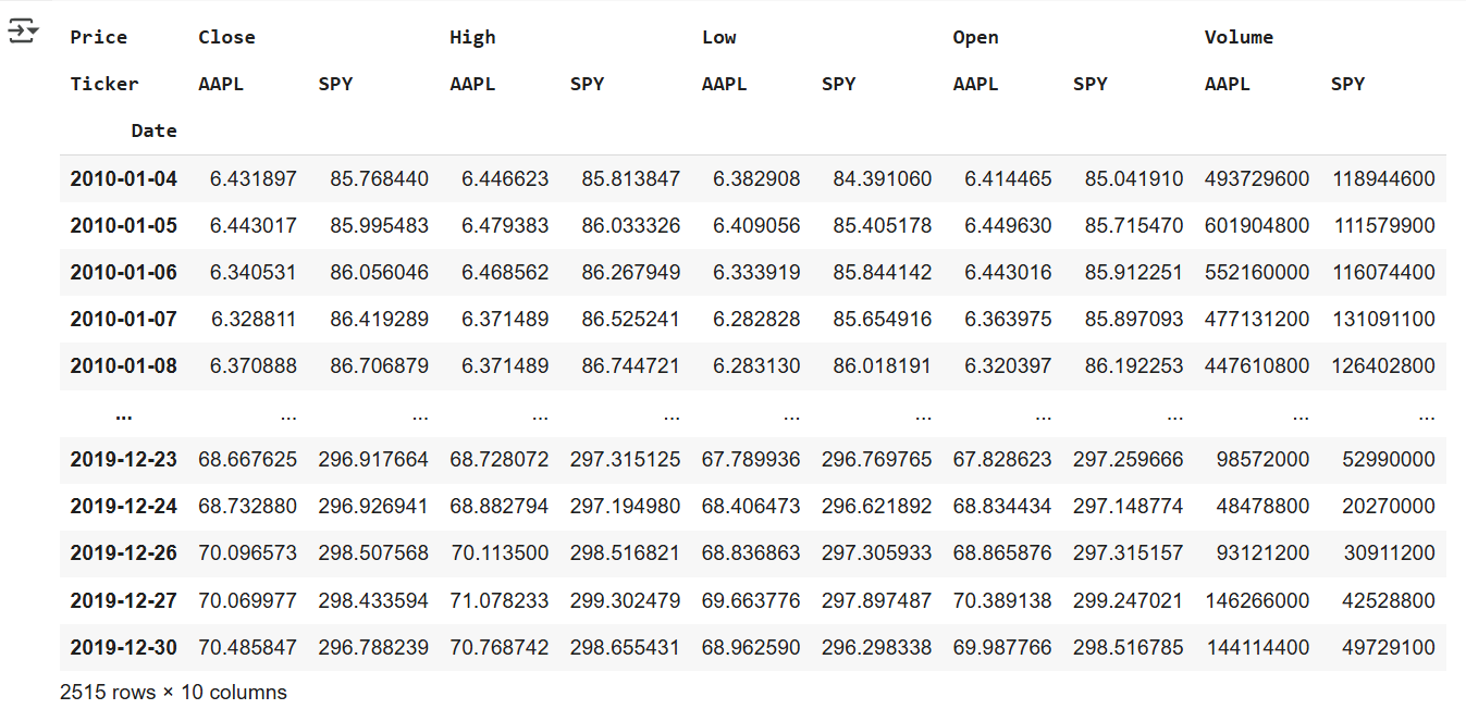
raw = yf.download('SPY AAPL', start='2010-01-01', end='2019-12-31')
raw
# Y Finance使用日期作为索引列, 每行代表一天。
# 查看列:这里有所谓的分层或多索引列,可以看到调整后的收盘价,因为我们同时要求苹果和标准普尔 500指数
# 所以我们在它下面有两个子列,可以看到收盘价、最高值、最低值、开盘价、 和Volumn
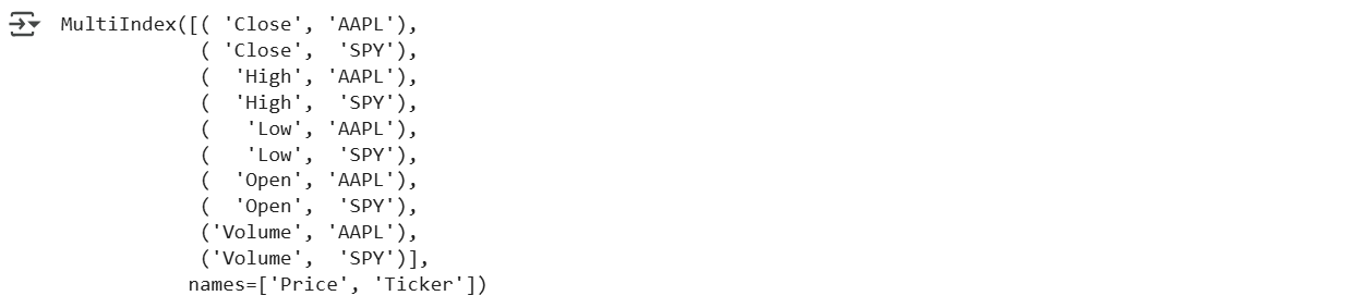
# 检查数据帧的columns属性
raw.columns
# 查看pipe的用法
raw.pipe?
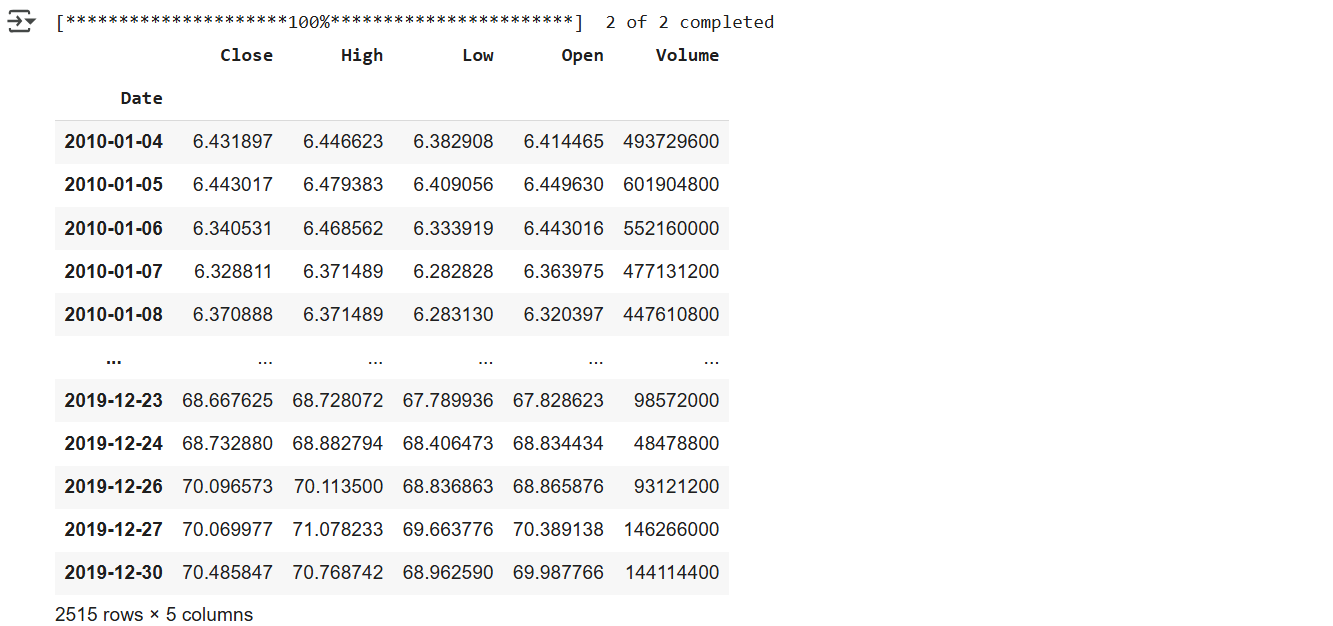
import yfinance as yf#fix_cols():重命名多层列索引为单层(只保留子列名)
def fix_cols(df):columns = df.columnsouter = [col[0] for col in columns]df.columns = outerreturn df# 加载与清洗逻辑封装在一个函数里,便于复用
def tweak_data():raw = yf.download('SPY AAPL',start='2010-01-01', end='2019-12-31')return (raw.iloc[:,::2].pipe(fix_cols)) # pipe():在链式调用中插入一个自定义函数。tweak_data()
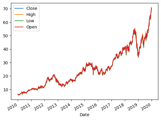
1.2. 折线图
创建线图,并整绘图的细节(如选择列、大小等)。
(raw.iloc[:,:-2:2] #从第0列开始,到倒数第2列,步长为2.pipe(fix_cols)
)
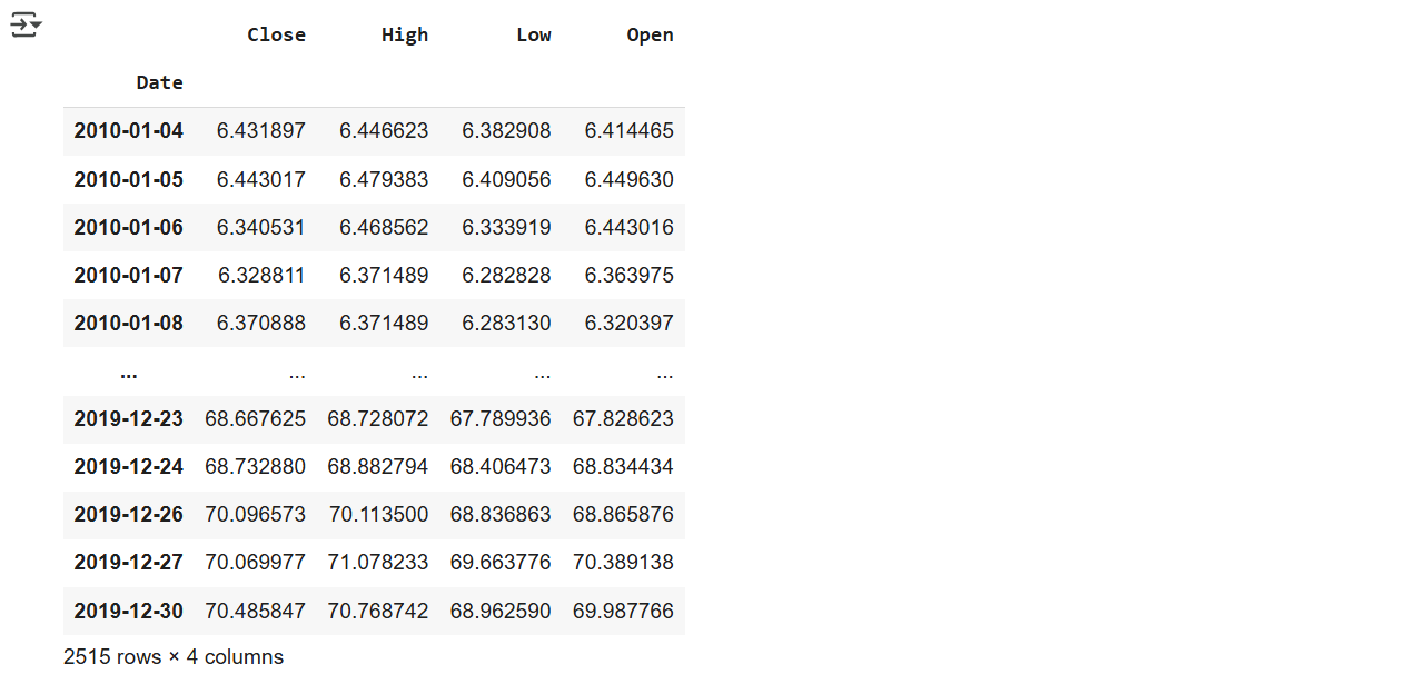
(raw.iloc[:,:-2:2].pipe(fix_cols).plot()
)
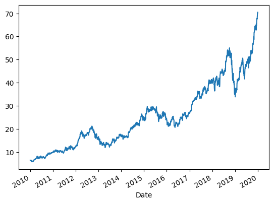
(raw.iloc[:,:-2:2].pipe(fix_cols).Close.plot()
)
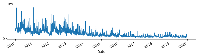
(raw.iloc[:,::2].pipe(fix_cols).Volume.plot(figsize=(10,2))  # 10英寸宽,2英寸高
)
1.3. 重采样
重新采样(resampling) 是将时间序列数据的频率从一个粒度转换为另一个粒度的过程,如从每日 → 每月,Pandas 提供了.resample() 方法。
(raw.iloc[:,::2].pipe(fix_cols).Close  # 每日收盘价.plot()
)
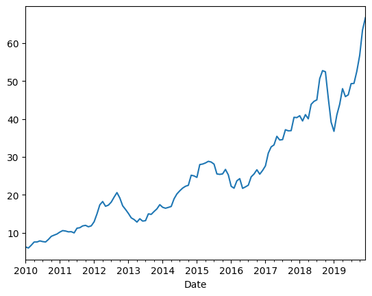
按月份分组:
(raw.iloc[:,::2].pipe(fix_cols).resample('M')  # offset alias.Close
)
(raw.iloc[:,::2].pipe(fix_cols).resample('M')  # offset alias.Close.mean().plot()  # 索引中有日期,列中有值,这样就可以绘制了
)
1.4. K线图 / 蜡烛图
fig, ax = plt.subplots(figsize=(10,5))
def plot_candle(df, ax):# wickax.vlines(x=df.index, ymin=df.Low, ymax=df.High, colors='k', linewidth=1)# red - decreasered = df.query('Open > Close')ax.vlines(x=red.index, ymin=red.Close, ymax=red.Open, colors='r', linewidth=3)# green - increasegreen = df.query('Open <= Close')ax.vlines(x=green.index, ymin=green.Close, ymax=green.Open, colors='g', linewidth=3)ax.xaxis.set_major_locator(dates.MonthLocator())ax.xaxis.set_major_formatter(dates.DateFormatter('%b-%y'))ax.xaxis.set_minor_locator(dates.DayLocator())return df(raw.iloc[:,::2].pipe(fix_cols).resample('d').agg({'Open':'first', 'High':'max', 'Low':'min', 'Close':'last'}).loc['jan 2018':'jun 2018'].pipe(plot_candle, ax)
)
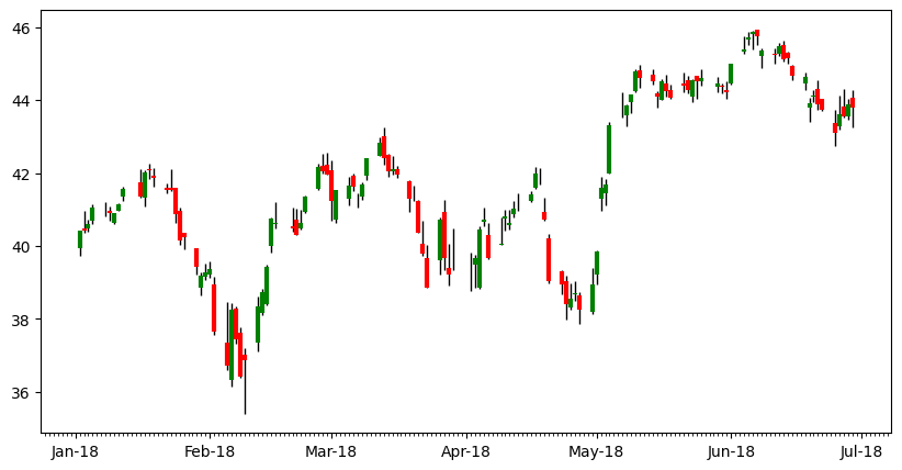
1.5. 挑战1
Plot the candles for the time period of Sep 2019 to Dec 2019. 可以做做看
2. 计算
Goal
- Explore Pandas methods like
.pct_change - Plotting with Pandas
- Refactoring to functions
2.1. 收益 / 回报
在金融中,“回报”通常指某个资产价格在两个时间点之间的相对变化。在Pandas中使用.pct_change() 方法计算百分比变化(Percentage Change),默认按前一行计算百分比变化(periods=1)。

# 使用aapl存储
aapl = (raw.iloc[:,::2].pipe(fix_cols))
aapl
# returns
aapl.pct_change()
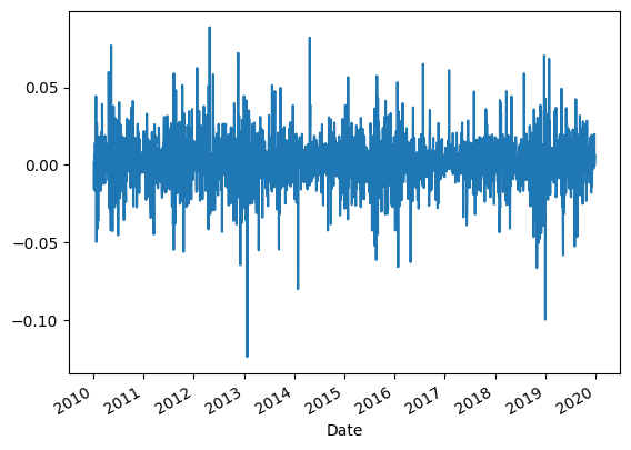
2.2. 绘制收益图
使用 .plot() 方法,查看回报的日常变化趋势。
# plot returns
(aapl.pct_change().Close.plot()
)
很多高频噪声,看起来像“毛毛虫”:
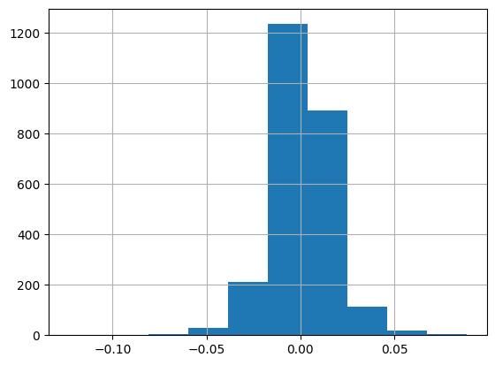
使用 .hist() 方法来观察回报的 分布情况(正负、极值、对称性等)。
# Histogram of Returns
(aapl.pct_change().Close.hist()
)
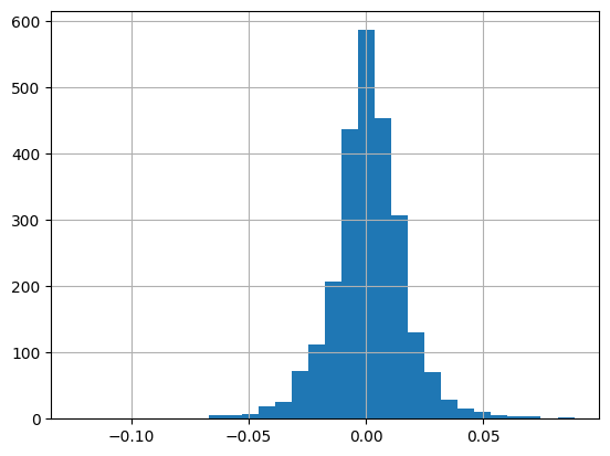
bins=30 表示分成 30 个区间,可以更细致地看到分布:
# Change bins
(aapl.pct_change().Close.hist(bins=30)
)
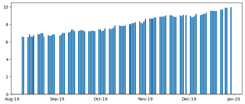
条形图用于查看一小段时间内每日的正负回报(比如最近 100 天):
# Understanding plotting in Pandas is a huge lever
# Bar Plot Returns
(aapl.pct_change().Close.iloc[-100:]  # 获取最后100个值.plot.bar()
)
Pandas 会把日期索引变成“分类变量”,导致 X 轴标签重叠、无法格式化。
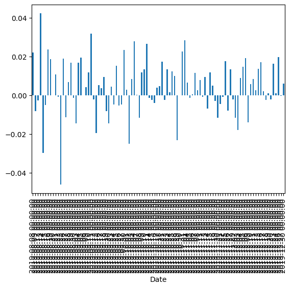
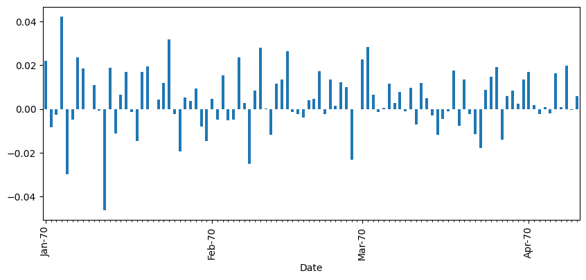
即使调整标签,也会显示成 1970-01 等错误日期:
# Bar Plot of Returns
# Sadly dates are broken with Pandas bar plots
# 1970s?
fig, ax = plt.subplots(figsize=(10, 4))
(aapl.pct_change().Close.iloc[-100:].plot.bar(ax=ax)
)
ax.xaxis.set_major_locator(dates.MonthLocator())
ax.xaxis.set_major_formatter(dates.DateFormatter('%b-%y'))
ax.xaxis.set_minor_locator(dates.DayLocator())
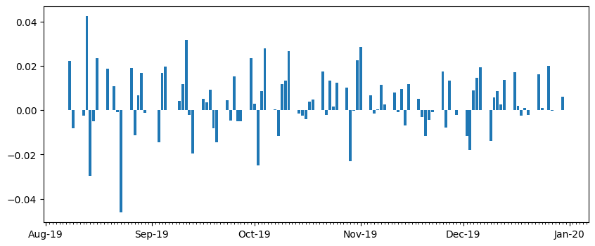
解决办法:使用 Matplotlib 手动绘制条形图
# Returns - using matplotlib
def my_bar(ser, ax):ax.bar(ser.index, ser)ax.xaxis.set_major_locator(dates.MonthLocator())ax.xaxis.set_major_formatter(dates.DateFormatter('%b-%y'))ax.xaxis.set_minor_locator(dates.DayLocator())return serfig, ax = plt.subplots(figsize=(10, 4))
_ = (aapl.pct_change().Close.iloc[-100:].pipe(my_bar, ax)
)
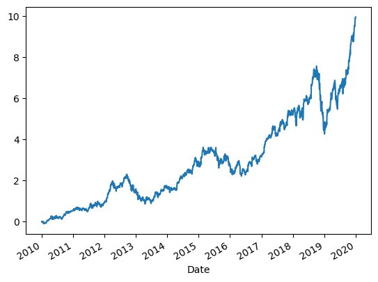
2.3. 累积收益
Goal:
- More complicated Pandas
- Refactoring into a function
- Explore source
- Creating new columns with
.assign - Illustrate lambda
Cumulative Returns is the amount that investment has gained or lost over time:
(current_price-original_price)/original_price
(aapl.Close.plot())
逐步计算:
(aapl.Close.sub(aapl.Close[0]) # substract.div(aapl.Close[0]) # divide.plot())
基于日收益的累积积:
# alternatte calculation
(aapl.Close # 取出收盘价序列.pct_change() # 计算日收益率(百分比变化).add(1)  # 转换为收益倍率 (1 + r).cumprod() # 计算累积乘积:累计收益倍率.sub(1) # 转换为累计收益率:累计倍率 - 1.plot() # 绘图 )
函数化重构:
# create a function for calculating
def calc_cum_returns(df,col):ser = df[col]return (ser.sub(ser[0]).div(ser[0]))
(aapl.pipe(calc_cum_returns,'Close').plot()
)
# Lambda is an *anonymous function*def get_returns(df):return calc_cum_returns(df,'Close')get_returns(aapl)
lambda这里我不太明白
(lambda df: get_returns(df))(aapl)
# Create a new column
(aapl.assign(cum_returns=lambda df: calc_cum_returns(df,'Close'))
)
# Returns - using matplotlib
def my_bar(ser, ax):ax.bar(ser.index, ser)ax.xaxis.set_major_locator(dates.MonthLocator())ax.xaxis.set_major_formatter(dates.DateFormatter('%b-%y'))ax.xaxis.set_minor_locator(dates.DayLocator())return serfig, ax = plt.subplots(figsize=(10, 4))
_ = (aapl
.pipe(calc_cum_returns, 'Close')
.iloc[-100:]
.pipe(my_bar, ax)
)
2.4. 波动率
Goals
- More complicated Pandas
- Learn about rolling operations
波动性(英语:volatility,又称波动率),指金融资产在一定时间段的变化性。在股票市场,以每天收市价计算的波动性称为历史波幅(Historical Volatility),以股票期权估算的未来波动性称为引申波幅(Implied Volatility)。着名的VIX指数是标准普尔500指数期权的30日引申波幅,以年度化表示。(维基百科)
(aapl.Close.mean()
)
(aapl.Close.std()
)
(aapl.assign(pct_change_close=aapl.Close.pct_change()).pct_change_close.std()
)
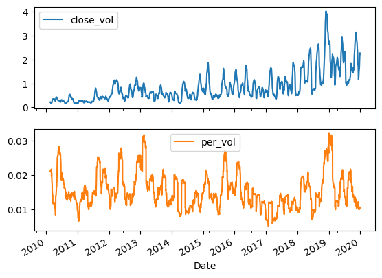
以滑动窗口方式计算“过去 N 天”的波动性:
(aapl.assign(close_vol=aapl.rolling(30).Close.std(),per_vol=aapl.Close.pct_change().rolling(30).std()).iloc[:,-2:].plot(subplots=True)
)
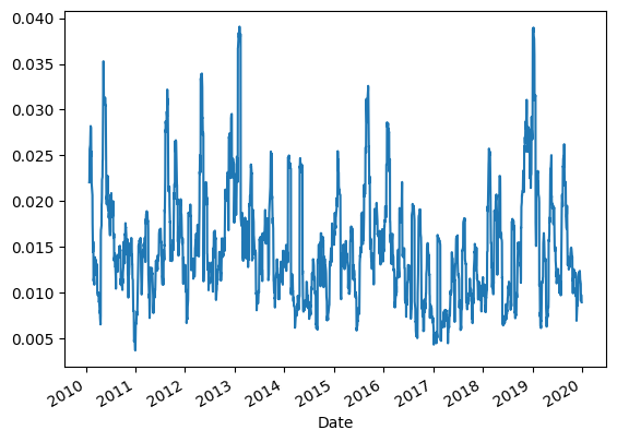
以固定周期(如每 15 天)进行分组计算标准差:
# 15 day volatility
(aapl.assign(pct_change_close=aapl.Close.pct_change()) # 创建一个名为百分比变化的列.resample('15D') # 15天为一个分组.std()
)
# 15 day rolling volatility
(aapl.assign(pct_change_close=aapl.Close.pct_change()) # 创建一个名为百分比变化的列.rolling(window=15, min_periods=15).std()
)
# 15 day volatility
# note if column name conflicts with method need to use
# index access ([])
(aapl.assign(pct_change=aapl.Close.pct_change()).rolling(window=15, min_periods=15).std()['pct_change'].plot())
2.5. 挑战2
Plot the rolling volatility over 30-day sliding windows for 2015-2019。(可以参考上面的代码)
3. 滚动窗口
3.1. 创建移动平均线
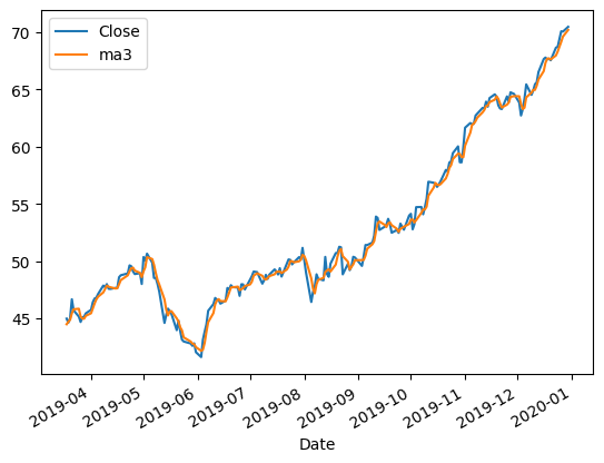
对苹果公司股票(aapl)的价格数据进行三日移动平均(ma3)的计算:
(aapl.assign(s1=aapl.Close.shift(1),s2=aapl.Close.shift(2),ma3=lambda df_:df_.loc[:, ['Close', 's1', 's2']].mean(axis='columns'),ma3_builtin=aapl.Close.rolling(3).mean())
)
3.2. 绘制移动平均线
(aapl.assign(s1=aapl.Close.shift(1),s2=aapl.Close.shift(2),ma3=lambda df_:df_.loc[:, ['Close', 's1', 's2']].mean(axis='columns'),ma3_builtin=aapl.Close.rolling(3).mean())[['Close','ma3']].iloc[-200:].plot()
)
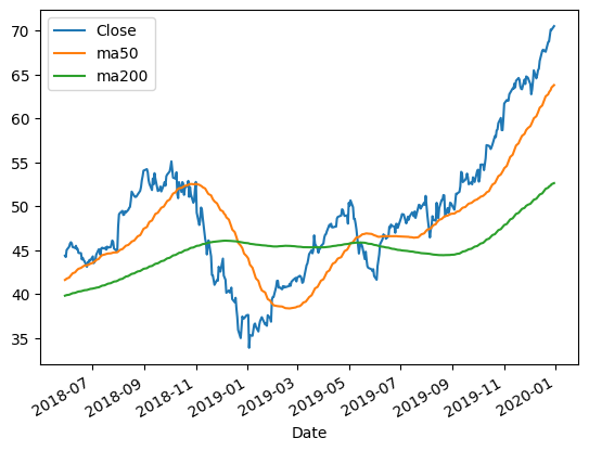
可视化苹果公司股票的收盘价与其 50 日、200 日移动平均线(MA):
(aapl.assign(ma50=aapl.Close.rolling(50).mean(),ma200=aapl.Close.rolling(200).mean(),)
[['Close', 'ma50', 'ma200']]
.iloc[-400:]
.plot()
)
如下图可以看到:Close(原始收盘价)是日常波动最明显的一条线;ma50是比较敏感的短期趋势线;而ma200是更平滑的长期趋势线。
3.3 Challenge
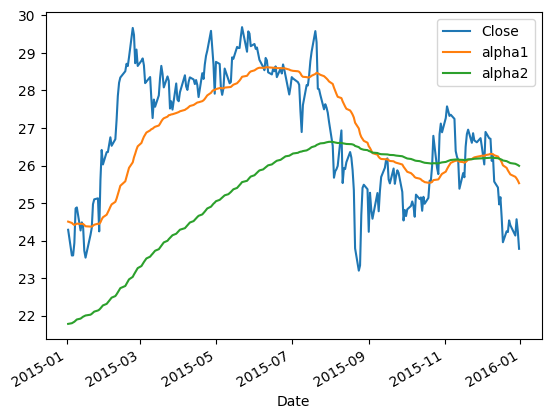
Create a plot with three lines:
- AAPL close price in 2015
- Exponential moving average with alpha =. 0392
- Exponential moving average with alpha =. 00995
Hint:Use the .ewm method to create a rolling aggregator.
aapl.ewm?
(aapl.loc['2015'].assign(alpha1=aapl.Close.ewm(alpha=0.0392).mean(),alpha2=aapl.Close.ewm(alpha=0.00995).mean(),)
[['Close', 'alpha1', 'alpha2']]
.plot()
)
alpha=0.0392:较高,表示更敏感,近期数据权重大,从而曲线更贴近原始价格;alpha=0.00995:较低,更平滑,趋势线更慢反应价格波动。
4. 技术分析
4.1. OBV
OBV(On-Balance Volume,能量潮指标),是一种常见的技术分析指标,用来结合价格走势和成交量判断趋势强度。OBV 是一个累加值:如果今日收盘价 > 昨日 → 当日成交量加到 OBV 上;如果今日收盘价 < 昨日 → 当日成交量从 OBV 中减去;如果收盘价不变 → OBV 保持不变,如下图:

下面函数的实现逻辑是对的,但是效率不高,会触发FutureWarning:
# naive
def calc_obv(df):df = df.copy()df["OBV"] = 0.0# Loop through the data and calculate OBVfor i in range(1, len(df)):# 如果该仓位的收盘价大于前一个收盘值if df["Close"][i] > df["Close"][i - 1]:df["OBV"][i]=df["OBV"][i - 1] + df["Volume"][i]elif df["Close"][i] < df["Close"][i - 1]:df["OBV"][i]=df["OBV"][i -1]-df["Volume"][i]else:df["OBV"][i] = df["OBV"][i - 1]return dfcalc_obv(aapl)
用 Pandas 向量化方式计算 OBV并使用 %timeit 测试:
%%timeit
# This is painful
(aapl.assign(close_prev=aapl.Close.shift(1),vol=0,obv=lambda adf: adf.vol.where(cond=adf.Close == adf.close_prev,other=adf.Volume.where(cond=adf.Close > adf.close_prev,other =- adf.Volume.where(cond=adf.Close < adf.close_prev, other=0))).cumsum())
)
用 np.select 实现 OBV 的向量化计算:
(aapl.assign(prev_close=aapl.Close.shift(1),vol=np.select([aapl.Close> aapl.Close.shift(1),aapl.Close == aapl.Close.shift(1),aapl.Close < aapl.Close.shift(1)],[aapl.Volume, 0, -aapl.Volume]),obv=lambda df_:df_. vol.cumsum(),)
)
将 OBV 的向量化计算封装成函数 calc_obv():
def calc_obv(df, close_col='Close', vol_col='Volume'):close = df[close_col]vol = df[vol_col]close_shift = close.shift(1)return (df.assign(vol=np.select([close > close_shift,close == close_shift,close < close_shift],[vol, 0, -vol]),obv=lambda df_:df_. vol.fillna(0).cumsum())['obv'])(aapl.assign(obv=calc_obv)
)
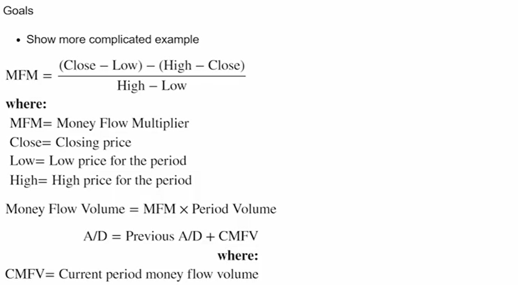
4.2. 累积/派发指标(A/D)
A/D 指标(Accumulation/Distribution Line,累积/派发线)是技术分析中衡量资金流入流出的常用指标之一。
- MFM(Money Flow Multiplier):资金流动乘数,用于衡量收盘价相对当天价格区间的位置,范围在[-1, 1],越接近 1 表示更靠近高点(资金流入),越接近 -1 表示更靠近低点(资金流出)。
- Money Flow Volume(资金流动量):把价格位置信息与成交量结合起来,收盘越靠近高点,且成交量越大,说明有更多资金“流入”。
- A/D 是一个累计值,用来判断市场是否处于吸筹(Accumulation)还是派发(Distribution)。
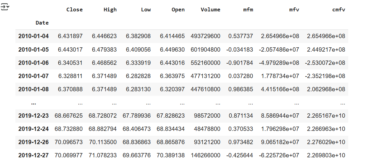
实现逻辑:
(aapl.assign(mfm=((aapl.Close - aapl.Low) - (aapl.High - aapl.Close))/(aapl.High - aapl.Low),mfv=lambda df_:df_.mfm * df_.Volume, # lambda将采用数据帧的当前值cmfv=lambda df_:df_.mfv.cumsum()))
# 重构为一个函数
def calc_ad(df, close_col='Close', low_col='Low', high_col='High',vol_col='Volume'):close = df[close_col]low = df[low_col]high = df[high_col]return (df.assign(mfm=((close - low) -(high - close))/(high - low),mfv=lambda df_: df_. mfm * df_[vol_col],cmfv=lambda df_: df_. mfv.cumsum()).cmfv
)(aapl.assign(ad=calc_ad).ad.plot()
)
 column. Relative Strength Index is a popular momentum indicator
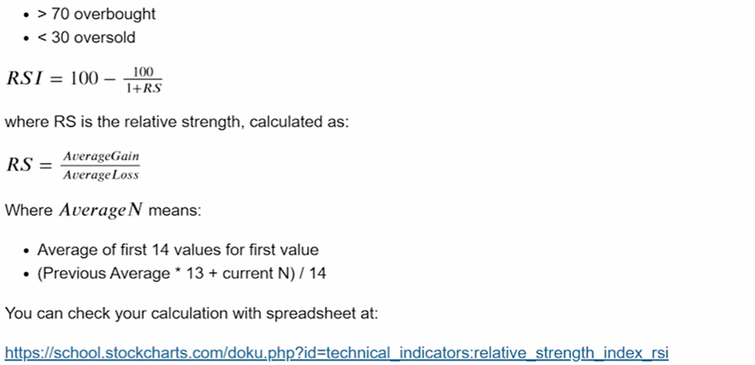
RSI(Relative Strength Index, 相对强弱指数)是一种常用的技术分析指标,用于衡量股票或其他资产价格的近期涨跌强度,帮助判断市场是否处于超买或超卖状态。RSI 的应用意义:
- 超买区:RSI 通常高于 70,意味着价格上涨过快,可能出现回调。
- 超卖区:RSI 通常低于 30,意味着价格下跌过快,可能出现反弹。
- 趋势判断:RSI 可以帮助确认价格趋势的强度和反转信号。
(aapl.assign(mfm=((aapl.Close - aapl.Low) - (aapl.High - aapl.Close))/(aapl.High - aapl.Low),mfv=lambda df_:df_.mfm * df_.Volume, # lambda将采用数据帧的当前值cmfv=lambda df_:df_.mfv.cumsum()))
# prompt: Create 14-day RSI columndef rsi(df: pd.DataFrame, window: int = 14) -> pd.DataFrame:"""Calculates the Relative Strength Index (RSI) for a given DataFrame.Args:df: The input DataFrame with a 'Close' column.window: The lookback window for RSI calculation (default is 14).Returns:The DataFrame with an added 'RSI' column."""delta = df['Close'].diff()up, down = delta.copy(), delta.copy()up[up < 0] = 0down[down > 0] = 0# Use rolling meanavg_gain = up.rolling(window=window).mean()avg_loss = abs(down.rolling(window=window).mean())rs = avg_gain / avg_lossdf['RSI'] = 100 - (100 / (1 + rs))return df.RSI# aapl = rsi(aapl)
# print(aapl.head(16))
(aapl.assign(rsi_14=rsi(aapl)).rsi_14# .plot()
)

相关文章:
【学习笔记】Python金融基础
Python金融入门 1. 加载数据与可视化1.1. 加载数据1.2. 折线图1.3. 重采样1.4. K线图 / 蜡烛图1.5. 挑战1 2. 计算2.1. 收益 / 回报2.2. 绘制收益图2.3. 累积收益2.4. 波动率2.5. 挑战2 3. 滚动窗口3.1. 创建移动平均线3.2. 绘制移动平均线3.3 Challenge 4. 技术分析4.1. OBV4.…...

在Linux查看电脑的GPU型号
VGA 是指 Video Graphics Array,这是 IBM 于 1987 年推出的一种视频显示标准。 lspci | grep vga 📌 lspci | grep -i vga 的含义 lspci:列出所有连接到 PCI 总线的设备。 grep -i vga:过滤输出,仅显示包含“VGA”字…...

A Execllent Software Project Review and Solutions
The Phoenix Projec: how do we produce software? how many steps? how many people? how much money? you will get it. i am a pretty judge of people…a prank...
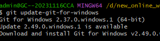
windows命令行面板升级Git版本
Date: 2025-06-05 11:41:56 author: lijianzhan Git 是一个 分布式版本控制系统 (DVCS),由 Linux 之父 Linus Torvalds 于 2005 年开发,用于管理 Linux 内核开发。它彻底改变了代码协作和版本管理的方式,现已成为软件开发的事实标准工具&…...

Langgraph实战--自定义embeding
概述 在Langgraph中我想使用第三方的embeding接口来实现文本的embeding。但目前langchain只提供了两个类,一个是AzureOpenAIEmbeddings,一个是:OpenAIEmbeddings。通过ChatOpenAI无法使用第三方的接口,例如:硅基流平台…...
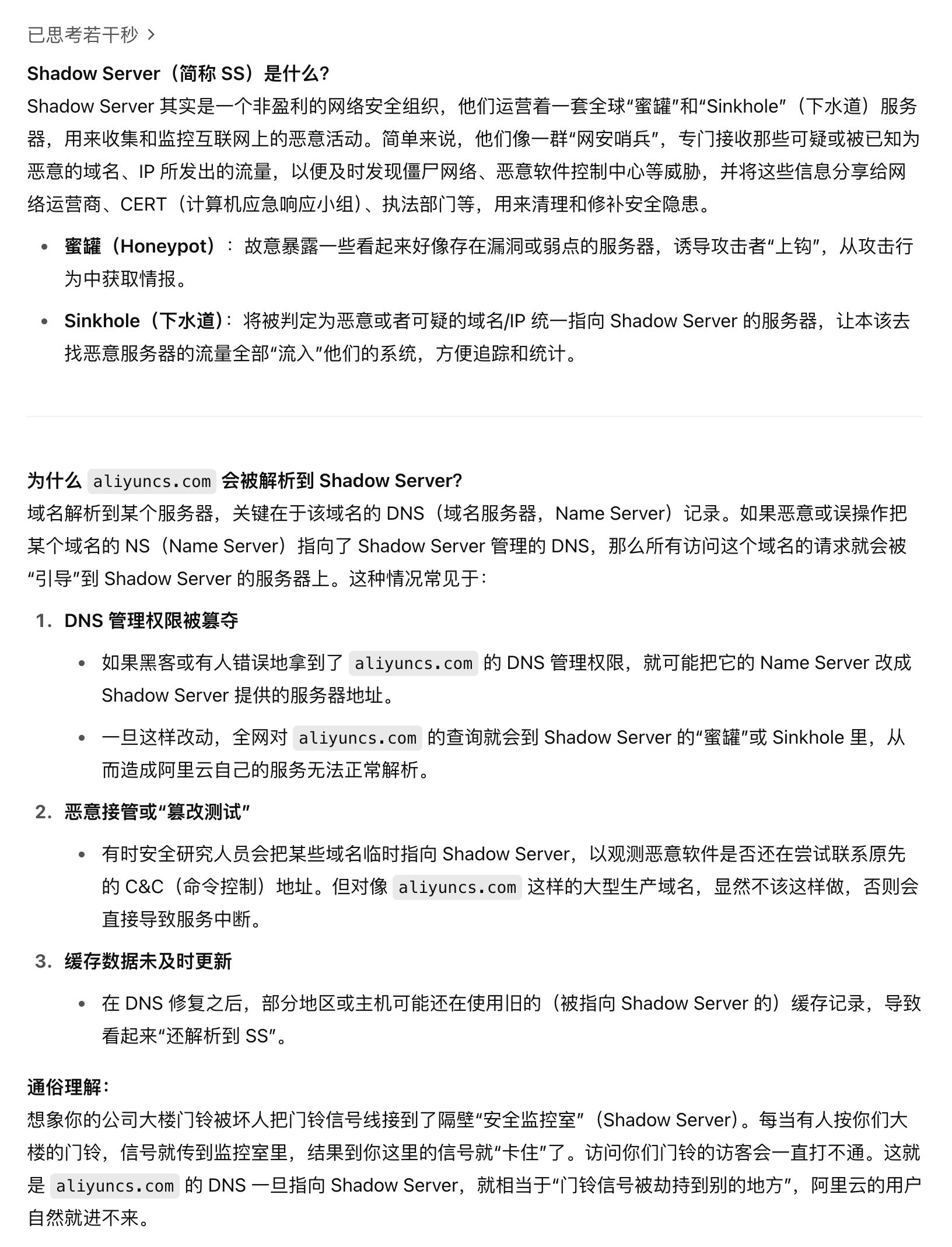
大故障,阿里云核心域名疑似被劫持
2025年6月5日凌晨,阿里云多个服务突发异常,罪魁祸首居然是它自家的“核心域名”——aliyuncs.com。包括对象存储 OSS、内容分发 CDN、镜像仓库 ACR、云解析 DNS 等服务在内,全部受到波及,用户业务连夜“塌房”。 更让人惊讶的是&…...
)
什么是「镜像」?(Docker Image)
🧊 什么是「镜像」?(Docker Image) 💡 人话解释: Docker 镜像就像是一个装好程序的“快照包”,里面包含了程序本体、依赖库、运行环境,甚至是系统文件。 你可以把镜像理解为&…...
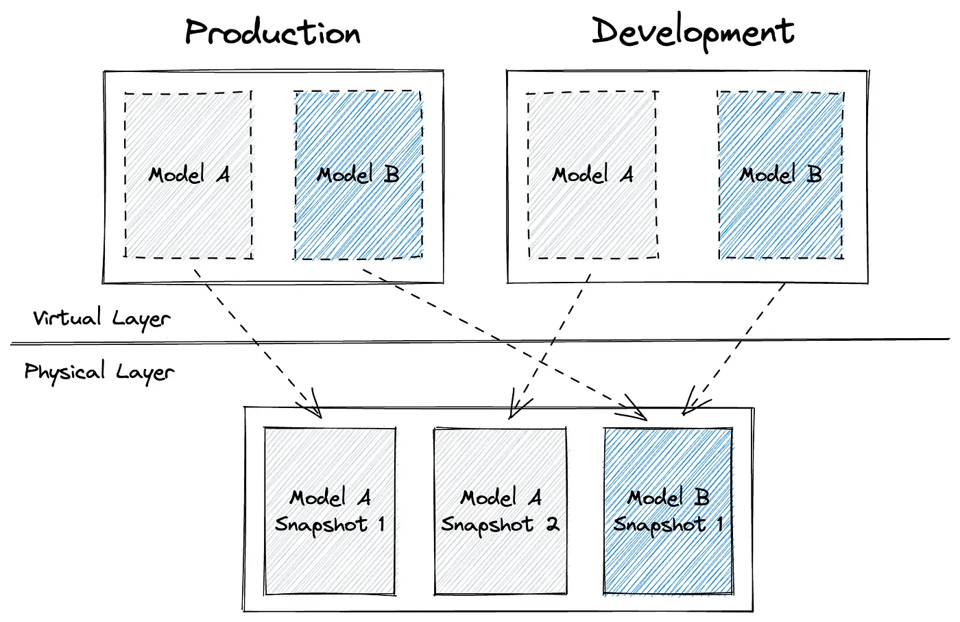
SQLMesh实战:用虚拟数据环境和自动化测试重新定义数据工程
在数据工程领域,软件工程实践(如版本控制、测试、CI/CD)的引入已成为趋势。尽管像 dbt 这样的工具已经推动了数据建模的标准化,但在测试自动化、工作流管理等方面仍存在不足。 SQLMesh 应运而生,旨在填补这些空白&…...

服务器健康摩尔斯电码:深度解读S0-S5状态指示灯
当服务器机柜中闪烁起神秘的琥珀色灯光,运维人员的神经瞬间绷紧——这些看似简单的Sx指示灯,实则是服务器用硬件语言发出的求救信号。掌握这套"摩尔斯电码",等于拥有了预判故障的透视眼。 一、状态指示灯:服务器的生命体…...
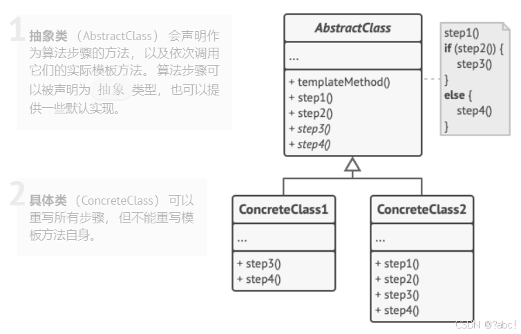
设计模式基础概念(行为模式):模板方法模式 (Template Method)
概述 模板方法模式是一种行为设计模式, 它在超类中定义了一个算法的框架, 允许子类在不修改结构的情况下重写算法的特定步骤。 是基于继承的代码复用的基本技术,模板方法模式的类结构图中,只有继承关系。 需要开发抽象类和具体子…...
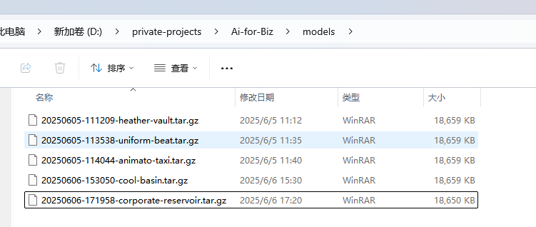
传统业务对接AI-AI编程框架-Rasa的业务应用实战(番外篇2)-- Rasa 训练数据文件的清理
经过我的【传统业务对接AI-AI编程框架-Rasa的业务应用实战】系列 1-6 的表述 已经实现了最初的目标:将传统平台业务(如发票开具、审核、计税、回款等)与智能交互结合,通过用户输入提示词或语音,识别用户意图和实体信…...

LVDS的几个关键电压概念
LVDS的几个关键电压概念 1.LVDS的直流偏置 直流偏置指的是信号的电压围绕的基准电压,信号的中心电压。在LVDS中,信号是差分的, 两根线之间的电压差表示数据,很多时候两根线的电压不是在0v开始变化的,而是在某个 固定的…...
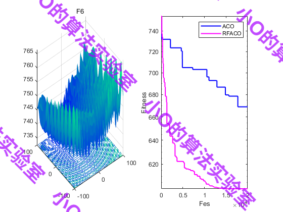
2023年ASOC SCI2区TOP,随机跟随蚁群优化算法RFACO,深度解析+性能实测
目录 1.摘要2.连续蚁群优化算法ACOR3.随机跟随策略4.结果展示5.参考文献6.代码获取7.算法辅导应用定制读者交流 1.摘要 连续蚁群优化是一种基于群体的启发式搜索算法(ACOR),其灵感来源于蚁群的路径寻找行为,具有结构简单、控制参…...
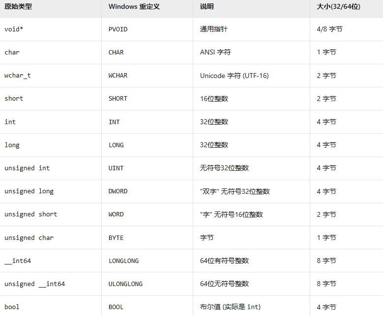
DLL动态库实现文件遍历功能(Windows编程)
源文件: 文件遍历功能的动态库,并支持用户注册回调函数处理遍历到的文件 a8f80ba 周不才/cpp_linux study - Gitee.com 知识准备 1.Windows中的数据类型 2.DLL导出/导入宏 使用__declspec(dllexport)修饰函数,将函数标记为导出函数存放到…...

Java Map完全指南:从基础到高级应用
文章目录 1. Map接口概述Map的基本特性 2. Map接口的核心方法基本操作方法批量操作方法 3. 主要实现类详解3.1 HashMap3.2 LinkedHashMap3.3 TreeMap3.4 ConcurrentHashMap 4. 高级特性和方法4.1 JDK 1.8新增方法4.2 Stream API结合使用 5. 性能比较和选择建议性能对比表选择建…...

jvm 垃圾收集算法 详解
垃圾收集算法 分代收集理论 垃圾收集器的理论基础,它建立在两个分代假说之上: 弱分代假说:绝大多数对象都是朝生夕灭的。强分代假说:熬过越多次垃圾收集过程的对象就越难以消亡。 这两个分代假说共同奠定了多款常用的垃圾收集…...
[特殊字符] 深入理解 Linux 内核进程管理:架构、核心函数与调度机制
Linux 内核作为一个多任务操作系统,其进程管理子系统是核心组成部分之一。无论是用户应用的运行、驱动行为的触发,还是系统调度决策,几乎所有操作都离不开进程的创建、调度与销毁。本文将从进程的概念出发,深入探讨 Linux 内核中进…...

Nginx Stream 层连接数限流实战ngx_stream_limit_conn_module
1.为什么需要连接数限流? 数据库/Redis/MQ 连接耗资源:恶意脚本或误配可能瞬间占满连接池,拖垮后端。防御慢速攻击:层叠式限速(连接数+带宽)可阻挡「Slow Loris」之类的 TCP 低速洪水。公平接入…...

Spring Boot 定时任务的使用
前言 在实际开发中,我们经常需要实现定时任务的功能,例如每天凌晨执行数据清理、定时发送邮件等。Spring Boot 提供了非常便捷的方式来实现定时任务,本文将详细介绍如何在 Spring Boot 中使用定时任务。 一、Spring Boot 定时任务简介 Spr…...
Flutter:下拉框选择
 文档地址dropdown_button2 // 限价、市价 状态final List<String> orderTypes [普通委托, 市价委托];String? selectedOrderType 普通委托;changeOrderType(String …...

SpringAI(GA):Nacos2下的分布式MCP
原文链接地址:SpringAI(GA):Nacos2下的分布式MCP 教程说明 说明:本教程将采用2025年5月20日正式的GA版,给出如下内容 核心功能模块的快速上手教程核心功能模块的源码级解读Spring ai alibaba增强的快速上手教程 源码级解读 版…...

AC68U刷梅林384/386版本后不能 降级回380,升降级解决办法
前些时间手贱更新了路由器的固件,384.18版本。结果发现了一堆问题,比如客户端列表加载不出来,软件中心打不开等等。想着再刷一下新的固件,结果死活刷不上去。最后翻阅了大量前辈的帖子找到了相关的处理办法。现在路由器中开启SSH&…...

[AI绘画]sd学习记录(二)文生图参数进阶
目录 7.高分辨率修复:以小博大8.细化器(Refiner):两模型接力9.随机数种子(Seed):复现图片吧 本文接续https://blog.csdn.net/qq_23220445/article/details/148460878?spm1001.2014.3001.5501…...

CRM管理系统中的客户分类与标签管理技巧:提升转化率的核心策略
在客户关系管理(CRM)领域,有效的客户分类与标签管理是提升销售效率、优化营销ROI的关键。据统计,使用CRM管理系统进行科学客户分层的企业,客户转化率平均提升35%(企销客数据)。本文将深入解析在CRM管理软件中实施客户分类与标签管理的最佳实践…...

怎么解决cesium加载模型太黑,程序崩溃,不显示,位置不对模型太大,Cesium加载gltf/glb模型后变暗
有时候咱们cesium加载模型时候型太黑,程序崩溃,不显示,位置不对模型太大怎么办 需要处理 可以联系Q:424081801 谢谢 需要处理 可以联系Q:424081801 谢谢...

【AI系列】BM25 与向量检索
博客目录 引言:信息检索技术的演进第一部分:BM25 算法详解第二部分:向量检索技术解析第三部分:BM25 与向量检索的对比分析第四部分:融合与创新:混合检索系统 引言:信息检索技术的演进 在信息爆…...

windows10搭建nfs服务器
windows10搭建nfs服务器 Windows10搭建NFS服务 - fuzidage - 博客园...

simulink这边重新第二次仿真时,直接UE5崩溃,然后simulink没有响应
提问 : simulink这边重新第二次仿真时,直接UE5崩溃,然后simulink没有响应 simulink和UE5仿真的时候,simulink这边先停止仿真(也就是官方要求的顺序——注意:如果先在UE5那边停止仿真,如果UE5这…...

react 常见的闭包陷阱深入解析
一、引子 先来看一段代码,你能说出这段代码的问题在哪吗? const [count, setCount] = useState(0); useEffect(() => {const timer = setTimeout(() => {setCount(count + 1);}, 1000);return () => clearTimeout(timer); }, []);正确答案: 这段代码存在闭包陷阱…...

【CATIA的二次开发22】关于抽象对象Document概念详细总结
在CATIA VBA开发中,Document对象是最核心、最基础的对象之一。它代表了当前在CATIA会话中打开的一个文档(文件)。 几乎所有与文件操作、模型访问相关的操作都始于获取一个Document对象。 一、Document对象概述 1、获取Document对象: 当前活动文档: 最常见的方式是获取用户…...