基于Pytorch框架的LSTM算法(二)——多维度单步预测
1.项目说明
**选用Close和Low两个特征,使用窗口time_steps窗口的2个特征,然后预测Close这一个特征数据未来一天的数据
当batch_first=True,则LSTM的inputs=(batch_size,time_steps,input_size)
batch_size = len(data)-time_steps
time_steps = 滑动窗口,本项目中值为lookback
input_size = 2【因为选取了Close和Low两个特征】**
2.数据集
参考:https://blog.csdn.net/qq_38633279/article/details/134245512?spm=1001.2014.3001.5501中的数据集
3.数据预处理
3.1 读取数据
import numpy as np
import pandas as pd
import matplotlib.pyplot as plt
import seaborn as sns
from sklearn.preprocessing import MinMaxScaler
import torch
import torch.nn as nn
import seaborn as sns
import math, time
from sklearn.metrics import mean_squared_errorfilepath = './data/rlData.csv'
data = pd.read_csv(filepath)
data = data.sort_values('Date')
data.head()
data.shapesns.set_style("darkgrid")
plt.figure(figsize = (15,9))
plt.plot(data[['Close']])
plt.xticks(range(0,data.shape[0],20), data['Date'].loc[::20], rotation=45)
plt.title("****** Stock Price",fontsize=18, fontweight='bold')
plt.xlabel('Date',fontsize=18)
plt.ylabel('Close Price (USD)',fontsize=18)
plt.show()
3.2 选取Close和Low两个特征
price = data[['Close', 'Low']]
3.3 数据归一化
scaler = MinMaxScaler(feature_range=(-1, 1))
price['Close'] = scaler.fit_transform(price['Close'].values.reshape(-1,1))
price['Low'] = scaler.fit_transform(price['Low'].values.reshape(-1,1))
3.4 数据集的制造[batch_size,time_steps,input_size]
本次选取2个维度特征作为输出,因此,input_size =2
x_train.shape = [batch_size,time_steps,input_size]
y_train.shape = [batch_size,1]
1. 输入选取的是Close和Low列作为多维度的输入,所以选择的是data数据中的第一列和第二列作为x_train【因此input_size=2】
2. 输出是选取的Close列作为预测,所以选取data数据的第一列作为y_train【即Close列作为y_train】。
#2.数据集的制作
def split_data(stock, lookback):data_raw = stock.to_numpy() data = []    for index in range(len(data_raw) - lookback): data.append(data_raw[index: index + lookback])data = np.array(data);test_set_size = int(np.round(0.2 * data.shape[0]))train_set_size = data.shape[0] - (test_set_size)x_train = data[:train_set_size,:-1,:]  #x_train.shape =  (198, 4, 2)y_train = data[:train_set_size,-1,0:1] #y_train.shape =  (198, 1)x_test = data[train_set_size:,:-1,:]   #x_test.shape =  (49, 4, 2)y_test = data[train_set_size:,-1,0:1]  #y_test.shape =  (49, 1)return [torch.Tensor(x_train), torch.Tensor(y_train), torch.Tensor(x_test),torch.Tensor(y_test)]lookback = 5
x_train, y_train, x_test, y_test = split_data(price, lookback)
print('x_train.shape = ',x_train.shape)
print('y_train.shape = ',y_train.shape)
print('x_test.shape = ',x_test.shape)
print('y_test.shape = ',y_test.shape)
4.LSTM算法
这里的LSTM算法和单维单步预测中的LSTM预测算法一模一样。只不过我们在制作数据集的时候,对于LSTM模型中输入不一样了。
class LSTM(nn.Module):def __init__(self, input_dim, hidden_dim, num_layers, output_dim):super(LSTM, self).__init__()self.hidden_dim = hidden_dimself.num_layers = num_layersself.lstm = nn.LSTM(input_dim, hidden_dim, num_layers, batch_first=True)self.fc = nn.Linear(hidden_dim, output_dim)def forward(self, x):h0 = torch.zeros(self.num_layers, x.size(0), self.hidden_dim).requires_grad_()c0 = torch.zeros(self.num_layers, x.size(0), self.hidden_dim).requires_grad_()out, (hn, cn) = self.lstm(x, (h0.detach(), c0.detach()))out = self.fc(out[:, -1, :])
5.预训练
input_dim = 2
hidden_dim = 32
num_layers = 2
output_dim = 1
num_epochs = 100model = LSTM(input_dim=input_dim, hidden_dim=hidden_dim, output_dim=output_dim, num_layers=num_layers)
criterion = torch.nn.MSELoss()
optimiser = torch.optim.Adam(model.parameters(), lr=0.01)hist = np.zeros(num_epochs)
lstm = []for t in range(num_epochs):y_train_pred = model(x_train)loss = criterion(y_train_pred, y_train)hist[t] = loss.item()# print("Epoch ", t, "MSE: ", loss.item())optimiser.zero_grad()loss.backward()optimiser.step()
6.绘制预测值和真实值拟合图形,以及loss图形
predict = pd.DataFrame(scaler.inverse_transform(y_train_pred.detach().numpy()))
original = pd.DataFrame(scaler.inverse_transform(y_train.detach().numpy()))sns.set_style("darkgrid")    fig = plt.figure()
fig.subplots_adjust(hspace=0.2, wspace=0.2)plt.subplot(1, 2, 1)
ax = sns.lineplot(x = original.index, y = original[0], label="Data", color='royalblue')
ax = sns.lineplot(x = predict.index, y = predict[0], label="Training Prediction (LSTM)", color='tomato')
ax.set_title('Stock price', size = 14, fontweight='bold')
ax.set_xlabel("Days", size = 14)
ax.set_ylabel("Cost (USD)", size = 14)
ax.set_xticklabels('', size=10)plt.subplot(1, 2, 2)
ax = sns.lineplot(data=hist, color='royalblue')
ax.set_xlabel("Epoch", size = 14)
ax.set_ylabel("Loss", size = 14)
ax.set_title("Training Loss", size = 14, fontweight='bold')
fig.set_figheight(6)
fig.set_figwidth(16)# make predictions
y_test_pred = model(x_test)# invert predictions
y_train_pred = scaler.inverse_transform(y_train_pred.detach().numpy())
y_train = scaler.inverse_transform(y_train.detach().numpy())
y_test_pred = scaler.inverse_transform(y_test_pred.detach().numpy())
y_test = scaler.inverse_transform(y_test.detach().numpy())# calculate root mean squared error
trainScore = math.sqrt(mean_squared_error(y_train[:,0], y_train_pred[:,0]))
print('Train Score: %.2f RMSE' % (trainScore))
testScore = math.sqrt(mean_squared_error(y_test[:,0], y_test_pred[:,0]))
print('Test Score: %.2f RMSE' % (testScore))
lstm.append(trainScore)
lstm.append(testScore)
lstm.append(training_time)
完整代码
问题描述:
选用Close和Low两个特征,使用窗口time_steps窗口的2个特征,然后预测Close这一个特征数据未来一天的数据
当batch_first=True,则LSTM的inputs=(batch_size,time_steps,input_size)
batch_size = len(data)-time_steps
time_steps = 滑动窗口,本项目中值为lookback
input_size = 2【因为选取了Close和Low两个特征】
#%%
import numpy as np
import pandas as pd
import matplotlib.pyplot as plt
import seaborn as sns
from sklearn.preprocessing import MinMaxScaler
import torch
import torch.nn as nn
import seaborn as sns
import math, time
from sklearn.metrics import mean_squared_errorfilepath = './data/rlData.csv'
data = pd.read_csv(filepath)
data = data.sort_values('Date')
data.head()
data.shapesns.set_style("darkgrid")
plt.figure(figsize = (15,9))
plt.plot(data[['Close']])
plt.xticks(range(0,data.shape[0],20), data['Date'].loc[::20], rotation=45)
plt.title("****** Stock Price",fontsize=18, fontweight='bold')
plt.xlabel('Date',fontsize=18)
plt.ylabel('Close Price (USD)',fontsize=18)
plt.show()#1.选取特征工程2个
price = data[['Close', 'Low']]scaler = MinMaxScaler(feature_range=(-1, 1))
price['Close'] = scaler.fit_transform(price['Close'].values.reshape(-1,1))
price['Low'] = scaler.fit_transform(price['Low'].values.reshape(-1,1))#2.数据集的制作
def split_data(stock, lookback):data_raw = stock.to_numpy() data = []    for index in range(len(data_raw) - lookback): data.append(data_raw[index: index + lookback])data = np.array(data);test_set_size = int(np.round(0.2 * data.shape[0]))train_set_size = data.shape[0] - (test_set_size)x_train = data[:train_set_size,:-1,:]  #x_train.shape =  (198, 4, 2)y_train = data[:train_set_size,-1,0:1] #y_train.shape =  (198, 1)x_test = data[train_set_size:,:-1,:]   #x_test.shape =  (49, 4, 2)y_test = data[train_set_size:,-1,0:1]  #y_test.shape =  (49, 1)return [torch.Tensor(x_train), torch.Tensor(y_train), torch.Tensor(x_test),torch.Tensor(y_test)]lookback = 5
x_train, y_train, x_test, y_test = split_data(price, lookback)
print('x_train.shape = ',x_train.shape)
print('y_train.shape = ',y_train.shape)
print('x_test.shape = ',x_test.shape)
print('y_test.shape = ',y_test.shape)class LSTM(nn.Module):def __init__(self, input_dim, hidden_dim, num_layers, output_dim):super(LSTM, self).__init__()self.hidden_dim = hidden_dimself.num_layers = num_layersself.lstm = nn.LSTM(input_dim, hidden_dim, num_layers, batch_first=True)self.fc = nn.Linear(hidden_dim, output_dim)def forward(self, x):h0 = torch.zeros(self.num_layers, x.size(0), self.hidden_dim).requires_grad_()c0 = torch.zeros(self.num_layers, x.size(0), self.hidden_dim).requires_grad_()out, (hn, cn) = self.lstm(x, (h0.detach(), c0.detach()))out = self.fc(out[:, -1, :]) return outinput_dim = 2
hidden_dim = 32
num_layers = 2
output_dim = 1
num_epochs = 100model = LSTM(input_dim=input_dim, hidden_dim=hidden_dim, output_dim=output_dim, num_layers=num_layers)
criterion = torch.nn.MSELoss()
optimiser = torch.optim.Adam(model.parameters(), lr=0.01)hist = np.zeros(num_epochs)
lstm = []for t in range(num_epochs):y_train_pred = model(x_train)loss = criterion(y_train_pred, y_train)hist[t] = loss.item()# print("Epoch ", t, "MSE: ", loss.item())optimiser.zero_grad()loss.backward()optimiser.step()predict = pd.DataFrame(scaler.inverse_transform(y_train_pred.detach().numpy()))
original = pd.DataFrame(scaler.inverse_transform(y_train.detach().numpy()))sns.set_style("darkgrid")    fig = plt.figure()
fig.subplots_adjust(hspace=0.2, wspace=0.2)plt.subplot(1, 2, 1)
ax = sns.lineplot(x = original.index, y = original[0], label="Data", color='royalblue')
ax = sns.lineplot(x = predict.index, y = predict[0], label="Training Prediction (LSTM)", color='tomato')
ax.set_title('Stock price', size = 14, fontweight='bold')
ax.set_xlabel("Days", size = 14)
ax.set_ylabel("Cost (USD)", size = 14)
ax.set_xticklabels('', size=10)plt.subplot(1, 2, 2)
ax = sns.lineplot(data=hist, color='royalblue')
ax.set_xlabel("Epoch", size = 14)
ax.set_ylabel("Loss", size = 14)
ax.set_title("Training Loss", size = 14, fontweight='bold')
fig.set_figheight(6)
fig.set_figwidth(16)# make predictions
y_test_pred = model(x_test)# invert predictions
y_train_pred = scaler.inverse_transform(y_train_pred.detach().numpy())
y_train = scaler.inverse_transform(y_train.detach().numpy())
y_test_pred = scaler.inverse_transform(y_test_pred.detach().numpy())
y_test = scaler.inverse_transform(y_test.detach().numpy())# calculate root mean squared error
trainScore = math.sqrt(mean_squared_error(y_train[:,0], y_train_pred[:,0]))
print('Train Score: %.2f RMSE' % (trainScore))
testScore = math.sqrt(mean_squared_error(y_test[:,0], y_test_pred[:,0]))
print('Test Score: %.2f RMSE' % (testScore))
lstm.append(trainScore)
lstm.append(testScore)
lstm.append(training_time)
参考:https://gitee.com/qiangchen_sh/stock-prediction/blob/master/%E4%BB%A3%E7%A0%81/LSTM%E4%BB%8E%E7%90%86%E8%AE%BA%E5%9F%BA%E7%A1%80%E5%88%B0%E4%BB%A3%E7%A0%81%E5%AE%9E%E6%88%98%204%20%E5%A4%9A%E7%BB%B4%E7%89%B9%E5%BE%81%E8%82%A1%E7%A5%A8%E4%BB%B7%E6%A0%BC%E9%A2%84%E6%B5%8B_Pytorch.ipynb
相关文章:
——多维度单步预测)
基于Pytorch框架的LSTM算法(二)——多维度单步预测
1.项目说明 **选用Close和Low两个特征,使用窗口time_steps窗口的2个特征,然后预测Close这一个特征数据未来一天的数据 当batch_firstTrue,则LSTM的inputs(batch_size,time_steps,input_size) batch_size len(data)-time_steps time_steps 滑动窗口&…...

cnn感受野计算方法
No. Layers Kernel Size Stride 1 Conv1 33 1 2 Pool1 22 2 3 Conv2 33 1 4 Pool2 22 2 5 Conv3 33 1 6 Conv4 33 1 7 Pool3 2*2 2 感受野初始值 l 0 1 l_0 1l 0 1,每层的感受野计算过程如下: l 0 1 l_0 1l 0 1 l 1 1 ( 3 − 1 ) 3 l_1 1…...

百分点科技受邀参加“第五届治理现代化论坛”
11月4日,由北京大学政府管理学院主办的“面向新时代的人才培养——第五届治理现代化论坛”举行,北京大学校党委常委、副校长、教务长王博,政府管理学院院长燕继荣参加开幕式并致辞,百分点科技董事长兼CEO苏萌受邀出席论坛…...

基于Springboot的智慧食堂设计与实现(有报告)。Javaee项目,springboot项目。
演示视频: 基于Springboot的智慧食堂设计与实现(有报告)。Javaee项目,springboot项目。 前些天发现了一个巨牛的人工智能学习网站,通俗易懂,风趣幽默,忍不住分享一下给大家。点击跳转到网站。 项…...
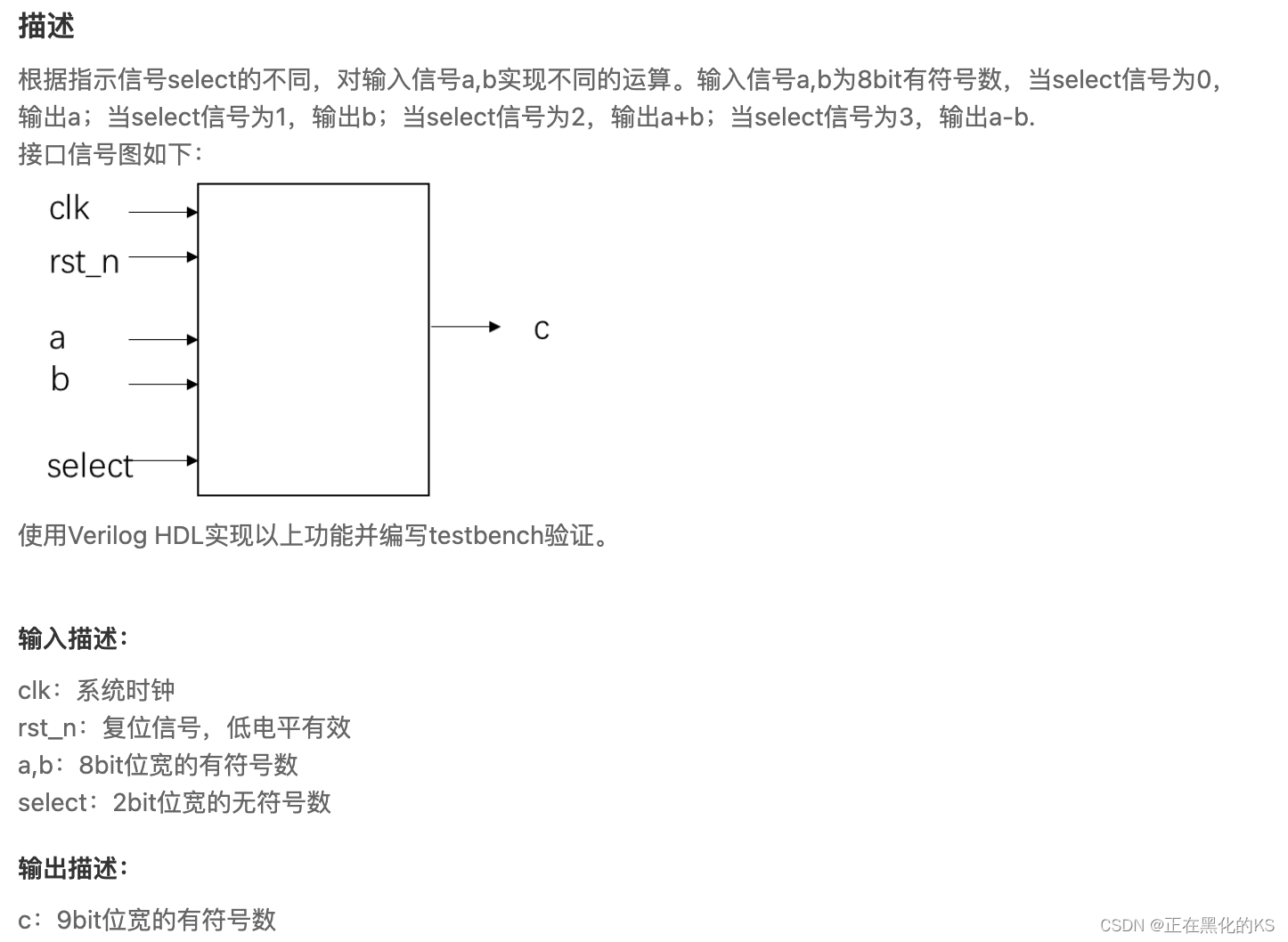
「Verilog学习笔记」多功能数据处理器
专栏前言 本专栏的内容主要是记录本人学习Verilog过程中的一些知识点,刷题网站用的是牛客网 分析 注意题目要求输入信号为有符号数,另外输出信号可能是输入信号的和,所以需要拓展一位,防止溢出。 timescale 1ns/1ns module data_…...

OpenHarmony 4.0 Release 编译异常处理
一、环境配置 编译环境:Ubuntu 20.04 OpenHarmony 软件版本:4.0 Release 设备平台:rk3568 二、下拉代码 参考官网步骤: OpenHarmony 4.0 Release 源码获取 repo init -u https://gitee.com/openharmony/manifest -b OpenHarmo…...

软件测试|MySQL LIKE:深入了解模糊查询
简介 在数据库查询中,模糊查询是一种强大的技术,可以用来搜索与指定模式匹配的数据。MySQL数据库提供了一个灵活而强大的LIKE操作符,使得模糊查询变得简单和高效。本文将详细介绍MySQL中的LIKE操作符以及它的用法,并通过示例演示…...

linux防火墙设置
#查看firewall的状态 firewall-cmd --state (systemctl status firewalld.service) #安装 yum install firewalld #启动, systemctl start firewalld (systemctl start firewalld.service) #设置开机启动 systemctl enable firewalld #关闭 systemctl stop firewalld #取消…...

http 403
一、什么是HTTP ERROR 403 403 Forbidden 是HTTP协议中的一个状态码(Status Code)。可以简单的理解为没有权限访问此站,服务器受到请求但拒绝提供服务。 二、HTTP 403 状态码解释大全 403.1 -执行访问禁止。 403.2 -读访问禁止。 403.3 -写访问禁止。 403.4要…...

RAW图像处理软件Capture One 23 Enterprise mac中文版功能特点
Capture One 23 Enterprise mac是一款专业的图像处理软件,旨在为企业用户提供高效、快速和灵活的工作流程。 Capture One 23 Enterprise mac软件的特点和功能 强大的图像编辑工具:Capture One 23 Enterprise提供了一系列强大的图像编辑工具,…...

Linux 进程终止和等待
目录 一:进程常见的退出方法 1. main 函数返回值 2.调用 exit 3.调用 _exit 二:异常问题 三:进程等待 1.概念 2.进程等待的必要性 3.进程等待的方法 <1>:wait --- 系统调用 <2>:waitpid 进程…...
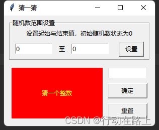
python用tkinter随机数猜数字大小
python用tkinter随机数猜数字大小 没事做,看到好多人用scratch做的猜大小的示例,也用python的tkinter搞一个猜大小的代码玩玩。 猜数字代码 from tkinter import * from random import randint# 定义确定按钮的点击事件 def hit(x,y):global s_Labprint(…...

程序员们保住自己饭碗
在现代社会中,程序员扮演着至关重要的角色。他们不仅仅是编写代码的人,更是保障数字世界安全稳定的守护者。随着科技的迅猛发展,程序员保住自己饭碗的护城河变得愈发重要。本文将探讨程序员如何通过不断学习、技术创新和软实力的发展…...

顶板事故防治vr实景交互体验提高操作人员安全防护技能水平
建筑业在我国各行业中属危险性较大且事故多发的行业,在建筑业“八大伤害”(高处坠落、坍塌、物体打击、触电、起重伤害、机械伤害、火灾爆炸及其他伤害)事故中,高处坠落事故的发生率最高、危险性极大。工地现场培训vr坠落体验利用虚拟现实技术还原各种情…...

为什么推荐从Linux开始了解IT技术
IT是什么,是干什么的呢? 说起物联网,云计算,大数据,或许大家听过。但是,你知道,像云计算的底层基座是什么呢?就是我们现在说的Linux操作系统。而云计算就是跑在Linux操作系统上的一个…...
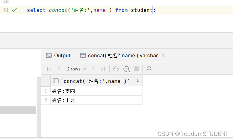
【Mysql】增删改查(基础版)
我使用的工具是Data Grip (SQLyog Naivact 都行) 使用Data Grip创建student表,具体步骤如下(熟悉Data Grip或者使用SQLyog,Naivact可以跳过) https://blog.csdn.net/m0_67930426/article/details/13429…...
文件夹找不到了怎么恢复?4个正确恢复方法分享!
“我在电脑上保存了很多的文件和文件夹,今天在查找文件时,发现我有一整个文件夹都消失了,不知道怎么才能找到呢。有朋友可以帮帮忙吗?” 电脑中文件夹突然找不到了可能会引发焦虑,尤其是如果这些文件夹包含重要的数据。…...
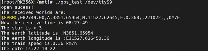
迅为RK3568开发板GPS模块测试实验步骤
1 首先按照上个实验-串口实验,在设备树中打开串口 9 的节点。 2 然后将 GPS 模块连接好之后,用 U 盘将 GPS 测试程序 gps_test 拷贝到开发板的/mnt 目录下。本小节的测试程序存放路径为“iTOP-3568 开发板\02_ 【iTOP-RK3568 开发板】开发资…...
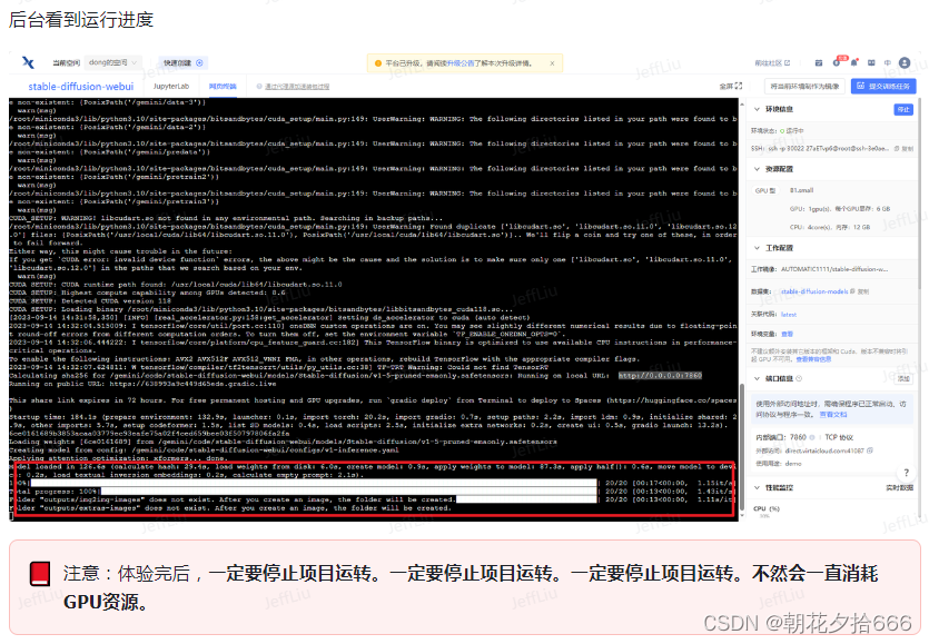
用趋动云GPU部署自己的Stable Diffusion
注:本文内容来自于对DataWhale的开源学习项目——免费GPU线上跑AI项目实践的学习,参见:Docs,引用了多处DataWhale给出的教程。 1.创建项目 1)进入趋动云用户工作台,在当前空间处选择注册时系统自动生成的…...
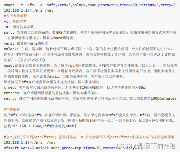
nfs配置
1.NFS介绍 NFS就是Network File System的缩写,它最大的功能就是可以通过网络,让不同的机器、不同的操 作系统可以共享彼此的文件。 NFS服务器可以让PC将网络中的NFS服务器共享的目录挂载到本地端的文 件系统中,而在本地端的系统中来看&#…...

JS如何通过WebUploader实现理赔视频的跨浏览器分片断点校验与压缩传输插件?
【一个被4G大文件逼疯的北京码农自述:如何在信创环境下优雅地让政府文件"飞"起来】 各位战友好,我是老张,北京某软件公司前端组"秃头突击队"队长。最近接了个政府项目,客户要求用国产环境上传4G大文件&#x…...

SwiftUI程序化导航与深度链接终极指南:Push通知和路由管理完全教程
SwiftUI程序化导航与深度链接终极指南:Push通知和路由管理完全教程 【免费下载链接】clean-architecture-swiftui SwiftUI sample app using Clean Architecture. Examples of working with SwiftData persistence, networking, dependency injection, unit testing…...

设计模式详解:建造者模式
一、概述建造者模式是一种创建型设计模式,它允许你分步骤地构建一个复杂的对象,而无需暴露其内部表示。换句话说,它把“构造”和“表示”分离,使得同样的构建过程可以创建出不同的对象。举个生活中的例子 🧩想象一下你…...

[具身智能-418]:URDF 文件详解
URDF(统一机器人描述格式)是机器人操作系统(ROS)中用于描述机器人模型的标准 XML 文件格式。你可以把它理解为机器人的“数字孪生说明书”,它精确地定义了机器人的物理结构、运动学关系、动力学参数和视觉外观…...

AI与SEO关键词优化的融合及其应用探索
在探讨AI与SEO关键词优化的融合时,本文将深入分析如何利用人工智能技术提升关键词研究的效率与准确性。首先,AI在分析用户搜索行为和意图方面展现出强大的能力,这使得关键词选择更加精准。其次,通过自然语言处理技术,A…...

2026年Hermes Agent/OpenClaw如何安装?阿里云及Coding Plan配置详细解读
2026年Hermes Agent/OpenClaw如何安装?阿里云及Coding Plan配置详细解读。OpenClaw(前身为Clawdbot/Moltbot)作为开源、本地优先的AI助理框架,凭借724小时在线响应、多任务自动化执行、跨平台协同等核心能力,成为个人办…...

构建高效JetBrains IDE评估重置机制的技术架构实现
构建高效JetBrains IDE评估重置机制的技术架构实现 【免费下载链接】ide-eval-resetter 项目地址: https://gitcode.com/gh_mirrors/id/ide-eval-resetter 在JetBrains IDE开发环境中,ide-eval-resetter项目通过智能评估信息清理技术,为开发者提…...

合约即契约,契约即性能:C++26 contracts如何让关键路径提速37%?——基于Linux内核模块级实测报告
第一章:合约即契约,契约即性能:C26 contracts如何让关键路径提速37%?——基于Linux内核模块级实测报告C26 引入的 [[assert: ...]] 和 [[expects: ...]] 合约机制,并非仅用于调试断言——其核心价值在于编译期可推导的…...
)
大模型训练实战:Attention与MoE层并行配置的5个关键调优技巧(附16卡实测数据)
大模型训练实战:Attention与MoE层并行配置的5个关键调优技巧(附16卡实测数据) 当你在16张A100上尝试训练千亿参数大模型时,最令人抓狂的往往不是代码bug,而是看着GPU利用率像心电图一样波动——某些卡满载到120℃时&am…...

基于MMC储能的分布式储能系统Simulink仿真及SOC均衡控制:模型预测控制在DC-DC升...
mmc储能 分布式储能simulink仿真 soc均衡控制 采用模型预测控制 dcdc升降压储能模块最近在搞MMC储能的仿真项目,发现这玩意儿真是电网调频的宝藏工具。特别是当分布式储能单元遇上模块化多电平换流器,SOC均衡控制就成了最烧脑的环节。今天咱们就撸起袖…...