[足式机器人]Part4 南科大高等机器人控制课 Ch03 Operator View of Rigid-Body Transformation
本文仅供学习使用
本文参考:
B站:CLEAR_LAB
笔者带更新-运动学
课程主讲教师:
Prof. Wei Zhang
南科大高等机器人控制课 Ch03 Operator View of Rigid-Body Transformation
- 1. Rotation Operation via Differential Equation
- 1.1 Skew Symmetric Matrices
- 1.2 Rotation Operation via Differential Equation
- 1.3 Raotation Matrix as a Rotation Operator
- 2. Rotation Operation in Different Frames
- 2.1 Rotation Martix Properties
- 2.2 Rotation Operation in Different Frames
- 3. Rigid-Body Operation via Diffeential Equation
- 3.1 SE(3)
- 3.2 se(3)
- 4. Homogeneous Transformation Matrix as Rigid-Body Operator
- 5. Rigid-Body Operation of Screw Axis
1. Rotation Operation via Differential Equation
1.1 Skew Symmetric Matrices
Recall that cross product is a special linear transformation.
For any ω ⃗ ∈ R 3 \vec{\omega}\in \mathbb{R} ^3 ω∈R3, there is a matrix ω ⃗ ~ ∈ R 3 × 3 \tilde{\vec{\omega}}\in \mathbb{R} ^{3\times 3} ω~∈R3×3 such that ω ⃗ × R ⃗ = ω ⃗ ~ R ⃗ \vec{\omega}\times \vec{R}=\tilde{\vec{\omega}}\vec{R} ω×R=ω~R
ω ⃗ = [ ω 1 ω 2 ω 3 ] ⟷ ω ⃗ ~ = [ 0 − ω 3 ω 2 ω 3 0 − ω 1 − ω 2 ω 1 0 ] \vec{\omega}=\left[ \begin{array}{c} \omega _1\\ \omega _2\\ \omega _3\\ \end{array} \right] \longleftrightarrow \tilde{\vec{\omega}}=\left[ \begin{matrix} 0& -\omega _3& \omega _2\\ \omega _3& 0& -\omega _1\\ -\omega _2& \omega _1& 0\\ \end{matrix} \right] ω= ω1ω2ω3 ⟷ω~= 0ω3−ω2−ω30ω1ω2−ω10
Note that a ⃗ ~ = − a ⃗ ~ T \tilde{\vec{a}}=-\tilde{\vec{a}}^{\mathrm{T}} a~=−a~T (called skew stmmetric)
ω ⃗ ~ \tilde{\vec{\omega}} ω~ is called a skew-symmetric matrix representation of the vector ω ⃗ \vec{\omega} ω
The set of skew-symmetric matrices in : s o ( n ) ≜ { S ∈ R n × n : S T = − S } so\left( n \right) \triangleq \left\{ S\in \mathbb{R} ^{n\times n}:S^{\mathrm{T}}=-S \right\} so(n)≜{S∈Rn×n:ST=−S}
We are interested in case n = 2 , 3 n=2,3 n=2,3
Rotation matrix ∈ S O ( 3 ) { R T R = E , det ( R ) = 1 } \in SO\left( 3 \right) \left\{ R^{\mathrm{T}}R=E,\det \left( R \right) =1 \right\} ∈SO(3){RTR=E,det(R)=1}
1.2 Rotation Operation via Differential Equation
- Consider a point initially located at R ⃗ p 0 \vec{R}_{p_0} Rp0 at time t = 0 t=0 t=0
- Rotate the point with unit angular velocity ω ^ \hat{\omega} ω^. Assuming the rotation axis passing through the origin, the motion is describe by
R ⃗ ˙ p ( t ) = ω ^ × R ⃗ p = ω ^ ~ R ⃗ p ( t ) , p ( 0 ) = p 0 \dot{\vec{R}}_p\left( t \right) =\hat{\omega}\times \vec{R}_p=\tilde{\hat{\omega}}\vec{R}_p\left( t \right) ,p\left( 0 \right) =p_0 R˙p(t)=ω^×Rp=ω^~Rp(t),p(0)=p0
linear velocity at time t t t, recall x ˙ = A x , x ( 0 ) = x 0 ⇒ x ( t ) = e A t x 0 \dot{x}=Ax,x\left( 0 \right) =x_0\Rightarrow x\left( t \right) =e^{At}x_0 x˙=Ax,x(0)=x0⇒x(t)=eAtx0 - This is a linear ODE with solution : R ⃗ ˙ p ( t ) = ω ^ ~ R ⃗ p ( t ) ⇒ R ⃗ ˙ p ( t ) = e ω ^ ~ t R ⃗ p 0 \dot{\vec{R}}_p\left( t \right) =\tilde{\hat{\omega}}\vec{R}_p\left( t \right) \Rightarrow \dot{\vec{R}}_p\left( t \right) =e^{\tilde{\hat{\omega}}t}\vec{R}_{p_0} R˙p(t)=ω^~Rp(t)⇒R˙p(t)=eω^~tRp0
- After t = θ t=\theta t=θ, the point has been rotated by θ \theta θ degree. Note R ⃗ ˙ p ( θ ) = e ω ^ ~ θ R ⃗ p 0 \dot{\vec{R}}_p\left( \theta \right) =e^{\tilde{\hat{\omega}}\theta}\vec{R}_{p_0} R˙p(θ)=eω^~θRp0, e ω ^ ~ θ e^{\tilde{\hat{\omega}}\theta} eω^~θ is rotation operator
- R o t ( ω ^ , θ ) ≜ e ω ^ ~ θ \mathrm{Rot}\left( \hat{\omega},\theta \right) \triangleq e^{\tilde{\hat{\omega}}\theta} Rot(ω^,θ)≜eω^~θ can be viewed as a rotation operator that rotates a point about ω ^ \hat{\omega} ω^ through θ \theta θ degree
The discussion holds for any reference frame
1.3 Raotation Matrix as a Rotation Operator
- Theorem: Every rotation matrix R R R can be written as R = R o t ( ω ^ , θ ) ≜ e ω ^ ~ θ ∈ S O ( 3 ) { R T R = E , det ( R ) = 1 } R=\mathrm{Rot}\left( \hat{\omega},\theta \right) \triangleq e^{\tilde{\hat{\omega}}\theta}\in SO\left( 3 \right) \left\{ R^{\mathrm{T}}R=E,\det \left( R \right) =1 \right\} R=Rot(ω^,θ)≜eω^~θ∈SO(3){RTR=E,det(R)=1}, i.e. , it represents a rotation operation about ω ^ \hat{\omega} ω^ by θ \theta θ
- We have seen how to use R R R to represent frame orientation and change of coordinate between different frames. They are quite different from the operator interpretation of R R R
- To apply the rotation operation, all the vectors / matrices have to be expressed in the same refrence frame
For example, assume R = [ 1 0 0 0 0 − 1 0 1 0 ] = R o t ( x ^ , π 2 ) R=\left[ \begin{matrix} 1& 0& 0\\ 0& 0& -1\\ 0& 1& 0\\ \end{matrix} \right] =\mathrm{Rot}\left( \hat{x},\frac{\pi}{2} \right) R= 1000010−10 =Rot(x^,2π)
Consider a relation q = R p q=Rp q=Rp:
- Change reference frame interpretation : two frames { A } , { B } \left\{ A \right\} ,\left\{ B \right\} {A},{B} , one physical Point a a a
R R R : orientation of { B } \left\{ B \right\} {B} relative to { A } \left\{ A \right\} {A} : i.e. R = [ Q B A ] R=\left[ Q_{\mathrm{B}}^{A} \right] R=[QBA]
then : p = a B , q = a A , q = R p ⇒ a A = [ Q B A ] a B p=a^B,q=a^A,q=Rp\Rightarrow a^A=\left[ Q_{\mathrm{B}}^{A} \right] a^B p=aB,q=aA,q=Rp⇒aA=[QBA]aB- Rotation operator interpretation : one frame and two points
a → a ′ , p = a A , q = a ′ A ⇒ a ′ A = R a A a\rightarrow a^{\prime},p=a^A,q={a^{\prime}}^A\Rightarrow {a^{\prime}}^A=Ra^A a→a′,p=aA,q=a′A⇒a′A=RaAConsider the frame operation:
- Change of reference frame :
Have one “frame object”, two reference frames
Frame object { A } \left\{ A \right\} {A}, orientation in { O } \left\{ O \right\} {O} , is R A O , R A B R_{\mathrm{A}}^{O},R_{\mathrm{A}}^{B} RAO,RAB, ⇒ R A O = R B O R A B = R R A B \Rightarrow R_{\mathrm{A}}^{O}=R_{\mathrm{B}}^{O}R_{\mathrm{A}}^{B}=RR_{\mathrm{A}}^{B} ⇒RAO=RBORAB=RRAB- Rotation a frame : R ′ A = R R A {R^{\prime}}_A=RR_A R′A=RRA
two frame objects, one refrence frame
more precisely : R ′ A = R R A ⇒ R A ′ O = R R A O {R^{\prime}}_A=RR_A\Rightarrow R_{\mathrm{A}^{\prime}}^{O}=RR_{\mathrm{A}}^{O} R′A=RRA⇒RA′O=RRAO
2. Rotation Operation in Different Frames
2.1 Rotation Martix Properties
[ Q ] [ Q ] T = E \left[ Q \right] \left[ Q \right] ^{\mathrm{T}}=E [Q][Q]T=E
[ Q 1 ] [ Q 2 ] ∈ S O ( 3 ) , i f [ Q 1 ] , [ Q 2 ] ∈ S O ( 3 ) \left[ Q_1 \right] \left[ Q_2 \right] \in SO\left( 3 \right) ,if\,\,\left[ Q_1 \right] ,\left[ Q_2 \right] \in SO\left( 3 \right) [Q1][Q2]∈SO(3),if[Q1],[Q2]∈SO(3): product of two rotation matrices is also a rotation matrix
p , q ∈ R 3 , ∥ [ Q ] R ⃗ p − [ Q ] R ⃗ q ∥ 2 = ∥ [ Q ] ( R ⃗ p − R ⃗ q ) ∥ 2 = ( R ⃗ p − R ⃗ q ) T [ Q ] T [ Q ] ( R ⃗ p − R ⃗ q ) = ∥ R ⃗ p − R ⃗ q ∥ 2 p,q\in \mathbb{R} ^3,\left\| \left[ Q \right] \vec{R}_p-\left[ Q \right] \vec{R}_{\mathrm{q}} \right\| ^2=\left\| \left[ Q \right] \left( \vec{R}_p-\vec{R}_{\mathrm{q}} \right) \right\| ^2=\left( \vec{R}_p-\vec{R}_{\mathrm{q}} \right) ^{\mathrm{T}}\left[ Q \right] ^{\mathrm{T}}\left[ Q \right] \left( \vec{R}_p-\vec{R}_{\mathrm{q}} \right) =\left\| \vec{R}_p-\vec{R}_{\mathrm{q}} \right\| ^2 p,q∈R3, [Q]Rp−[Q]Rq 2= [Q](Rp−Rq) 2=(Rp−Rq)T[Q]T[Q](Rp−Rq)= Rp−Rq 2
∥ R ⃗ p − R ⃗ q ∥ = ∥ [ Q ] R ⃗ p − [ Q ] R ⃗ q ∥ \left\| \vec{R}_p-\vec{R}_{\mathrm{q}} \right\| =\left\| \left[ Q \right] \vec{R}_p-\left[ Q \right] \vec{R}_{\mathrm{q}} \right\| Rp−Rq = [Q]Rp−[Q]Rq : rotation operator preserves distance
[ Q ] ( v ⃗ × w ⃗ ) = [ Q ] v ⃗ × [ Q ] w ⃗ \left[ Q \right] \left( \vec{v}\times \vec{w} \right) =\left[ Q \right] \vec{v}\times \left[ Q \right] \vec{w} [Q](v×w)=[Q]v×[Q]w
[ Q ] w ⃗ ~ [ Q ] T = [ Q ] w ⃗ ~ \left[ Q \right] \tilde{\vec{w}}\left[ Q \right] ^{\mathrm{T}}=\widetilde{\left[ Q \right] \vec{w}} [Q]w~[Q]T=[Q]w —— important
2.2 Rotation Operation in Different Frames
Consider two frames { A } \left\{ A \right\} {A} and { B } \left\{ B \right\} {B}, the actual numerical values of the operator R o t ( ω ^ , θ ) \mathrm{Rot}\left( \hat{\omega},\theta \right) Rot(ω^,θ) depend on both the reference frame to repersent ω ^ \hat{\omega} ω^ and the reference frame to represent the operator itself
Consider a rotation axis ω ^ \hat{\omega} ω^ (coordinate free vector), with { A } \left\{ A \right\} {A} - frame coordinate ω ^ A \hat{\omega}^A ω^A and { B } \left\{ B \right\} {B} - frame. We know ω ⃗ A = [ Q B A ] ω ⃗ B \vec{\omega}^A=\left[ Q_{\mathrm{B}}^{A} \right] \vec{\omega}^B ωA=[QBA]ωB
Let B R o t ( B ω ^ , θ ) ^B\mathrm{Rot}\left( ^B\hat{\omega},\theta \right) BRot(Bω^,θ) and A R o t ( A ω ^ , θ ) ^A\mathrm{Rot}\left( ^A\hat{\omega},\theta \right) ARot(Aω^,θ) be the two rotation matrices, representing the same rotation operatioon R o t ( ω ^ , θ ) \mathrm{Rot}\left( \hat{\omega},\theta \right) Rot(ω^,θ) in frames { A } \left\{ A \right\} {A} and { B } \left\{ B \right\} {B}
We have the relation : A R o t ( A ω ^ , θ ) = [ Q B A ] B R o t ( B ω ^ , θ ) [ Q A B ] ^A\mathrm{Rot}\left( ^A\hat{\omega},\theta \right) =\left[ Q_{\mathrm{B}}^{A} \right] ^B\mathrm{Rot}\left( ^B\hat{\omega},\theta \right) \left[ Q_{\mathrm{A}}^{B} \right] ARot(Aω^,θ)=[QBA]BRot(Bω^,θ)[QAB]
-
Approach 1 : two points p → p ′ ⇒ R ⃗ p ′ A = A R o t ( A ω ^ , θ ) R ⃗ p A p\rightarrow p^{\prime}\Rightarrow \vec{R}_{\mathrm{p}^{\prime}}^{A}=^A\mathrm{Rot}\left( ^A\hat{\omega},\theta \right) \vec{R}_{\mathrm{p}}^{A} p→p′⇒Rp′A=ARot(Aω^,θ)RpA
{ B } \left\{ B \right\} {B} - frame : R ⃗ p ′ B = B R o t ( B ω ^ , θ ) R ⃗ p B \vec{R}_{\mathrm{p}^{\prime}}^{B}=^B\mathrm{Rot}\left( ^B\hat{\omega},\theta \right) \vec{R}_{\mathrm{p}}^{B} Rp′B=BRot(Bω^,θ)RpB
⇒ [ Q B A ] R ⃗ p ′ B = [ Q B A ] B R o t ( B ω ^ , θ ) R ⃗ p B ⇒ R ⃗ p ′ A = [ Q B A ] B R o t ( B ω ^ , θ ) [ Q B A ] R ⃗ p A ⇒ A R o t ( A ω ^ , θ ) = [ Q B A ] B R o t ( B ω ^ , θ ) [ Q B A ] \Rightarrow \left[ Q_{\mathrm{B}}^{A} \right] \vec{R}_{\mathrm{p}^{\prime}}^{B}=\left[ Q_{\mathrm{B}}^{A} \right] ^B\mathrm{Rot}\left( ^B\hat{\omega},\theta \right) \vec{R}_{\mathrm{p}}^{B}\Rightarrow \vec{R}_{\mathrm{p}^{\prime}}^{A}=\left[ Q_{\mathrm{B}}^{A} \right] ^B\mathrm{Rot}\left( ^B\hat{\omega},\theta \right) \left[ Q_{\mathrm{B}}^{A} \right] \vec{R}_{\mathrm{p}}^{A}\Rightarrow ^A\mathrm{Rot}\left( ^A\hat{\omega},\theta \right) =\left[ Q_{\mathrm{B}}^{A} \right] ^B\mathrm{Rot}\left( ^B\hat{\omega},\theta \right) \left[ Q_{\mathrm{B}}^{A} \right] ⇒[QBA]Rp′B=[QBA]BRot(Bω^,θ)RpB⇒Rp′A=[QBA]BRot(Bω^,θ)[QBA]RpA⇒ARot(Aω^,θ)=[QBA]BRot(Bω^,θ)[QBA] -
Approach 2 : for a ⃗ ∈ R 3 , a ⃗ ~ ∈ s o ( 3 ) , [ Q ] ∈ S O ( 3 ) \vec{a}\in \mathbb{R} ^3,\tilde{\vec{a}}\in so\left( 3 \right) ,\left[ Q \right] \in SO\left( 3 \right) a∈R3,a~∈so(3),[Q]∈SO(3)
⇒ [ Q ] a ⃗ ∈ R 3 , [ Q ] a ⃗ ~ = [ Q ] a ⃗ ~ [ Q ] T \Rightarrow \left[ Q \right] \vec{a}\in \mathbb{R} ^3,\widetilde{\left[ Q \right] \vec{a}}=\left[ Q \right] \tilde{\vec{a}}\left[ Q \right] ^{\mathrm{T}} ⇒[Q]a∈R3,[Q]a =[Q]a~[Q]T
R o t ( ω ⃗ A , θ ) = e ω ⃗ ~ A θ = e [ Q B A ] ω ⃗ B ~ θ = e [ Q B A ] ω ⃗ ~ B [ Q B A ] T θ = [ Q B A ] e ω ⃗ ~ B θ [ Q B A ] T ← e P A P − 1 = P e A P − 1 Rot\left( \vec{\omega}^A,\theta \right) =e^{\tilde{\vec{\omega}}^A\theta}=e^{\widetilde{\left[ Q_{\mathrm{B}}^{A} \right] \vec{\omega}^B}\theta}=e^{\left[ Q_{\mathrm{B}}^{A} \right] \tilde{\vec{\omega}}^B\left[ Q_{\mathrm{B}}^{A} \right] ^{\mathrm{T}}\theta}=\left[ Q_{\mathrm{B}}^{A} \right] e^{\tilde{\vec{\omega}}^B\theta}\left[ Q_{\mathrm{B}}^{A} \right] ^{\mathrm{T}}\gets e^{PAP^{-1}}=Pe^AP^{-1} Rot(ωA,θ)=eω~Aθ=e[QBA]ωB θ=e[QBA]ω~B[QBA]Tθ=[QBA]eω~Bθ[QBA]T←ePAP−1=PeAP−1
3. Rigid-Body Operation via Diffeential Equation
Recall: Every [ Q ] ∈ S O ( 3 ) \left[ Q \right] \in SO\left( 3 \right) [Q]∈SO(3) can be viewed as the state transition matrix associated with the rotation ODE(1). It maps the initial position to the current position(after the rotation motion)
- p ⃗ ( θ ) = R o t ( ω ⃗ , θ ) p ⃗ 0 \vec{p}\left( \theta \right) =Rot\left( \vec{\omega},\theta \right) \vec{p}_0 p(θ)=Rot(ω,θ)p0 viewed as solution to p ⃗ ˙ ( t ) = ω ⃗ ~ p ⃗ ( t ) , p ⃗ ( 0 ) = p ⃗ 0 \dot{\vec{p}}\left( t \right) =\tilde{\vec{\omega}}\vec{p}\left( t \right) ,\vec{p}\left( 0 \right) =\vec{p}_0 p˙(t)=ω~p(t),p(0)=p0 at t = θ t=\theta t=θ
- The above relation requires that the rotation axis passes through the origin.
We can obtain similar ODE characterization for [ T ] ∈ S E ( 3 ) \left[ T \right] \in SE\left( 3 \right) [T]∈SE(3) , which will lead to exponential coordinate of SE(3)
Recall : Theorem (Chasles): Every rigid body motion can be realized by a screw motion
Consider a point p p p undergoes a screw motion with screw axis S \mathcal{S} S and unit speed ( θ ˙ = 1 \dot{\theta}=1 θ˙=1). Let the cooresponding twist be V = θ ˙ S = ( ω ⃗ , v ⃗ ) \mathcal{V} =\dot{\theta}\mathcal{S} =\left( \vec{\omega},\vec{v} \right) V=θ˙S=(ω,v) . The motion can be described be the following ODE.
p ⃗ ˙ ( t ) = ω ⃗ × p ⃗ ( t ) + v ⃗ ⇒ [ p ⃗ ˙ ( t ) 0 ] = [ ω ⃗ ~ v ⃗ 0 0 ] [ p ⃗ ( t ) 1 ] \dot{\vec{p}}\left( t \right) =\vec{\omega}\times \vec{p}\left( t \right) +\vec{v}\Rightarrow \left[ \begin{array}{c} \dot{\vec{p}}\left( t \right)\\ 0\\ \end{array} \right] =\left[ \begin{matrix} \tilde{\vec{\omega}}& \vec{v}\\ 0& 0\\ \end{matrix} \right] \left[ \begin{array}{c} \vec{p}\left( t \right)\\ 1\\ \end{array} \right] p˙(t)=ω×p(t)+v⇒[p˙(t)0]=[ω~0v0][p(t)1]
Solution in homogeneous coordinate is :
[ p ⃗ ( t ) 1 ] = exp ( [ ω ⃗ ~ v ⃗ 0 0 ] t ) [ p ⃗ ( 0 ) 1 ] \left[ \begin{array}{c} \vec{p}\left( t \right)\\ 1\\ \end{array} \right] =\exp \left( \left[ \begin{matrix} \tilde{\vec{\omega}}& \vec{v}\\ 0& 0\\ \end{matrix} \right] t \right) \left[ \begin{array}{c} \vec{p}\left( 0 \right)\\ 1\\ \end{array} \right] [p(t)1]=exp([ω~0v0]t)[p(0)1]
3.1 SE(3)
For any twist V = ( ω ⃗ , v ⃗ ) \mathcal{V} =\left( \vec{\omega},\vec{v} \right) V=(ω,v), let [ V ] \left[ \mathcal{V} \right] [V] be its matrix representation of twist V \mathcal{V} V
[ V ] = [ ω ⃗ ~ v ⃗ 0 0 ] ∈ R 4 × 4 \left[ \mathcal{V} \right] =\left[ \begin{matrix} \tilde{\vec{\omega}}& \vec{v}\\ 0& 0\\ \end{matrix} \right] \in \mathbb{R} ^{4\times 4} [V]=[ω~0v0]∈R4×4
-
The abve definition also applies to a screw axis S = ( ω ⃗ , v ⃗ ) , [ S ] = [ ω ⃗ ~ v ⃗ 0 0 ] \mathcal{S} =\left( \vec{\omega},\vec{v} \right) ,\left[ \mathcal{S} \right] =\left[ \begin{matrix} \tilde{\vec{\omega}}& \vec{v}\\ 0& 0\\ \end{matrix} \right] S=(ω,v),[S]=[ω~0v0]
-
With this notation, the solution is [ p ⃗ ( t ) 1 ] = e [ S ] t [ p ⃗ ( 0 ) 1 ] \left[ \begin{array}{c} \vec{p}\left( t \right)\\ 1\\ \end{array} \right] =e^{\left[ \mathcal{S} \right] t}\left[ \begin{array}{c} \vec{p}\left( 0 \right)\\ 1\\ \end{array} \right] [p(t)1]=e[S]t[p(0)1]
-
Fact: e [ S ] t ∈ S E ( 3 ) e^{\left[ \mathcal{S} \right] t}\in SE\left( 3 \right) e[S]t∈SE(3) is always a valid homogeneous transformation matrix.
[ T ] = e [ S ] t = [ [ Q ] R ⃗ 0 1 ] \left[ T \right] =e^{\left[ \mathcal{S} \right] t}=\left[ \begin{matrix} \left[ Q \right]& \vec{R}\\ 0& 1\\ \end{matrix} \right] [T]=e[S]t=[[Q]0R1] -
Fact: Any T ∈ S E ( 3 ) T\in SE\left( 3 \right) T∈SE(3) can be written as [ T ] = e [ S ] t \left[ T \right] =e^{\left[ \mathcal{S} \right] t} [T]=e[S]t, i.e. , it can be viewed as an operator that moves a point/frame along the screw axis S \mathcal{S} S at unit speed for time t t t
3.2 se(3)
∀ ω ⃗ ∈ R 3 → ω ⃗ ~ ∈ s o ( 3 ) → e ω ⃗ ~ θ ∈ S O ( 3 ) ∀ S ∈ R 6 → [ S ] ∣ 4 × 4 = [ ω ⃗ ~ v ⃗ 0 0 ] ∈ s e ( 3 ) → e [ S ] θ ∈ S E ( 3 ) \forall \vec{\omega}\in \mathbb{R} ^3\rightarrow \tilde{\vec{\omega}}\in so\left( 3 \right) \rightarrow e^{\tilde{\vec{\omega}}\theta}\in SO\left( 3 \right) \\ \forall \mathcal{S} \in \mathbb{R} ^6\rightarrow \left. \left[ \mathcal{S} \right] \right|_{4\times 4}=\left[ \begin{matrix} \tilde{\vec{\omega}}& \vec{v}\\ 0& 0\\ \end{matrix} \right] \in se\left( 3 \right) \rightarrow e^{\left[ \mathcal{S} \right] \theta}\in SE\left( 3 \right) ∀ω∈R3→ω~∈so(3)→eω~θ∈SO(3)∀S∈R6→[S]∣4×4=[ω~0v0]∈se(3)→e[S]θ∈SE(3)
Similar to s o ( 3 ) so\left( 3 \right) so(3) , we can define s e ( 3 ) se\left( 3 \right) se(3) :
s e ( 3 ) = { ( ω ⃗ ~ , v ⃗ ) , ω ⃗ ~ ∈ s o ( 3 ) , v ⃗ ∈ R 3 } se\left( 3 \right) =\left\{ \left( \tilde{\vec{\omega}},\vec{v} \right) ,\tilde{\vec{\omega}}\in so\left( 3 \right) ,\vec{v}\in \mathbb{R} ^3 \right\} se(3)={(ω~,v),ω~∈so(3),v∈R3}
- s e ( 3 ) se\left( 3 \right) se(3) contains all matrix representation of twists or equivalently all twists.
- In some references, [ V ] \left[ \mathcal{V} \right] [V] is called a twist
- Sometimes, we may abuse notation by writing V ∈ s e ( 3 ) \mathcal{V} \in se\left( 3 \right) V∈se(3)
4. Homogeneous Transformation Matrix as Rigid-Body Operator
-
ODE for rigid motion under V = ( ω ⃗ , v ⃗ ) \mathcal{V} =\left( \vec{\omega},\vec{v} \right) V=(ω,v)
p ⃗ ˙ = v ⃗ + ω ⃗ × p ⃗ ⇒ [ p ⃗ ˙ 0 ] = [ ω ⃗ ~ v ⃗ 0 0 ] [ p ⃗ 1 ] ⇒ [ p ⃗ ˙ 0 ] = e [ V ] t [ p ⃗ 1 ] \dot{\vec{p}}=\vec{v}+\vec{\omega}\times \vec{p}\Rightarrow \left[ \begin{array}{c} \dot{\vec{p}}\\ 0\\ \end{array} \right] =\left[ \begin{matrix} \tilde{\vec{\omega}}& \vec{v}\\ 0& 0\\ \end{matrix} \right] \left[ \begin{array}{c} \vec{p}\\ 1\\ \end{array} \right] \Rightarrow \left[ \begin{array}{c} \dot{\vec{p}}\\ 0\\ \end{array} \right] =e^{\left[ \mathcal{V} \right] t}\left[ \begin{array}{c} \vec{p}\\ 1\\ \end{array} \right] p˙=v+ω×p⇒[p˙0]=[ω~0v0][p1]⇒[p˙0]=e[V]t[p1] -
Consider “unit velocity” V = S \mathcal{V} =\mathcal{S} V=S, then time t t t means degree
if not unit speed : V = θ ˙ S \mathcal{V} =\dot{\theta}\mathcal{S} V=θ˙S -
[ p ⃗ ′ 1 ] = [ T ] [ p ⃗ 1 ] \left[ \begin{array}{c} \vec{p}^{\prime}\\ 1\\ \end{array} \right] =\left[ T \right] \left[ \begin{array}{c} \vec{p}\\ 1\\ \end{array} \right] [p′1]=[T][p1] : “rotate” p ⃗ \vec{p} p about screw axis S \mathcal{S} S by θ \theta θ degree
[ T ] = e [ S ] θ \left[ T \right] =e^{\left[ \mathcal{S} \right] \theta} [T]=e[S]θ, two points : [ p ⃗ 1 ] → [ p ⃗ ′ 1 ] \left[ \begin{array}{c} \vec{p}\\ 1\\ \end{array} \right] \rightarrow \left[ \begin{array}{c} \vec{p}^{\prime}\\ 1\\ \end{array} \right] [p1]→[p′1] , more precisely : [ p ⃗ O ′ 1 ] = [ T O ] [ p ⃗ O 1 ] \left[ \begin{array}{c} {\vec{p}^O}^{\prime}\\ 1\\ \end{array} \right] =\left[ T^O \right] \left[ \begin{array}{c} \vec{p}^O\\ 1\\ \end{array} \right] [pO′1]=[TO][pO1]
For [ T ] ∈ S E ( 3 ) \left[ T \right] \in SE\left( 3 \right) [T]∈SE(3) config representative [ T B A ] \left[ T_{\mathrm{B}}^{A} \right] [TBA] : config of { B } \left\{ B \right\} {B} relative to { A } \left\{ A \right\} {A} —— [ p ⃗ A 1 ] = [ T B A ] [ p ⃗ B 1 ] \left[ \begin{array}{c} \vec{p}^A\\ 1\\ \end{array} \right] =\left[ T_{\mathrm{B}}^{A} \right] \left[ \begin{array}{c} \vec{p}^B\\ 1\\ \end{array} \right] [pA1]=[TBA][pB1]——same physical point but two different frames -
[ T ] [ T A ] \left[ T \right] \left[ T_A \right] [T][TA] : “rotate” { A } \left\{ A \right\} {A}-frame about S \mathcal{S} S by θ \theta θ degree
Rigid-Body Operator in Different Frames
Expression of [ T ] \left[ T \right] [T] in another frame (other than { O } \left\{ O \right\} {O}):
[ T O ] ↔ [ T B O ] − 1 [ T O ] [ T B O ] \left[ T^O \right] \leftrightarrow \left[ T_{\mathrm{B}}^{O} \right] ^{-1}\left[ T^O \right] \left[ T_{\mathrm{B}}^{O} \right] [TO]↔[TBO]−1[TO][TBO]
5. Rigid-Body Operation of Screw Axis
Consider an arbitrary screw axis S \mathcal{S} S , suppose the axis has gone through a rigid transformation [ T ] = ( [ Q ] , R ⃗ ) \left[ T \right] =\left( \left[ Q \right] ,\vec{R} \right) [T]=([Q],R) and the resulting new screw axis is S ′ \mathcal{S} ^{\prime} S′ , then
S ′ = [ A d T ] S \mathcal{S} ^{\prime}=\left[ Ad_T \right] \mathcal{S} S′=[AdT]S
Let’s work an arbitrary frame { A } \left\{ A \right\} {A} (rigidly attached to the screw axis)
Let { B } \left\{ B \right\} {B} be the frame obtained be apply [ T ] \left[ T \right] [T] operation
the coordinate of S \mathcal{S} S in { A } \left\{ A \right\} {A} is the same as the coordinate of S ′ \mathcal{S} ^{\prime} S′ in { B } \left\{ B \right\} {B} : S A = S ′ B \mathcal{S} ^A={\mathcal{S} ^{\prime}}^B SA=S′B
We also know [ T B ] = [ T ] [ T A ] , [ T ] = [ T B A ] \left[ T_B \right] =\left[ T \right] \left[ T_{\mathrm{A}} \right] ,\left[ T \right] =\left[ T_{\mathrm{B}}^{A} \right] [TB]=[T][TA],[T]=[TBA]
Multiply [ X B A ] \left[ X_{\mathrm{B}}^{A} \right] [XBA] : ⇒ [ X B A ] S A = [ X B A ] S ′ B = S ′ A ⇒ S ′ A = [ X B A ] S A \Rightarrow \left[ X_{\mathrm{B}}^{A} \right] \mathcal{S} ^A=\left[ X_{\mathrm{B}}^{A} \right] {\mathcal{S} ^{\prime}}^B={\mathcal{S} ^{\prime}}^A\Rightarrow {\mathcal{S} ^{\prime}}^A=\left[ X_{\mathrm{B}}^{A} \right] \mathcal{S} ^A ⇒[XBA]SA=[XBA]S′B=S′A⇒S′A=[XBA]SA
[ X B A ] = [ [ Q B A ] 0 R ⃗ ~ B A [ Q B A ] [ Q B A ] ] = [ A d T ] \left[ X_{\mathrm{B}}^{A} \right] =\left[ \begin{matrix} \left[ Q_{\mathrm{B}}^{A} \right]& 0\\ \tilde{\vec{R}}_{\mathrm{B}}^{A}\left[ Q_{\mathrm{B}}^{A} \right]& \left[ Q_{\mathrm{B}}^{A} \right]\\ \end{matrix} \right] =\left[ Ad_T \right] [XBA]=[[QBA]R~BA[QBA]0[QBA]]=[AdT]
1
2
3
4
5
6
7
8
9
相关文章:
[足式机器人]Part4 南科大高等机器人控制课 Ch03 Operator View of Rigid-Body Transformation
本文仅供学习使用 本文参考: B站:CLEAR_LAB 笔者带更新-运动学 课程主讲教师: Prof. Wei Zhang 南科大高等机器人控制课 Ch03 Operator View of Rigid-Body Transformation 1. Rotation Operation via Differential Equation1.1 Skew Symmetr…...
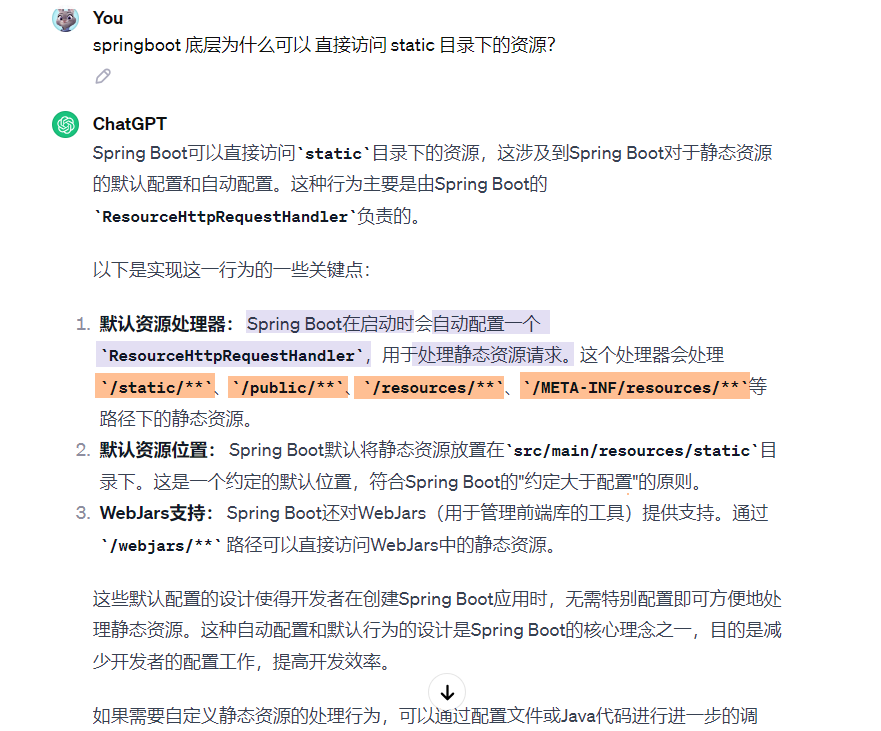
SpringBoot项目静态资源默认访问目录
SpringBoot项目:静态资源默认访问目录 参考博客:https://blog.csdn.net/weixin_43808717/article/details/118281904...

xtu oj 1255 勾股数
题目描述 勾股数是指满足a2b2c2的正整数,比如最有名的“勾三股四弦五”。 现在给你两个正整数,请问是否存在另外一个正整数,使其成为“勾股数”? 输入 第一行是一个整数K,表示样例的个数。 以后每行一个样例,为两个…...

【ArcGIS Pro微课1000例】0051:创建数据最小几何边界范围(点、线、面数据均可)
本实例为专栏系统文章:创建点数据最小几何边界(范围),配套案例数据,持续同步更新! 文章目录 一、工具介绍二、实战演练三、注意事项一、工具介绍 创建包含若干面的要素类,用以表示封闭单个输入要素或成组的输入要素指定的最小边界几何。 工具界面及参数如下所示: 核心…...

Oracle 怎樣修改DB_NAME
DBNEWID 是一个数据库实用程序,用于更改 Oracle 数据库的 DBNAME 和 DBID。可以更改 DBID 或 DBNAME 或两者。 DBNAME 是在创建数据库时指定的数据库名称,DBID 是创建数据库时分配给数据库的唯一编号。 以下步骤演示如何使用 DBNEWID 实用程序更改 Oracl…...

git标签的管理与思考
git 标签管理 git 如何打标签呢? 标签是什么? 标签 相当于一个 版本管理的一个贴纸,随时 可以通过标签 切换到 这个版本的状态 , 有人可能有疑问 git commit 就可以知道 代码的改动了, 为啥还需要标签来管理呢? …...
)
ESP32网络编程-OTA方式升级固件(基于Arduino IDE)
OTA方式升级固件(基于Arduino IDE) 文章目录 OTA方式升级固件(基于Arduino IDE)1、ESP32的OTA介绍2、OTA升级固件方式3、软件准备4、硬件准备5、代码实现ESP32吸引人的编程方式之一就是通过OTA方式升级固件。本文将详细介绍在Arduino IDE中升级固件。 1、ESP32的OTA介绍 O…...

力扣-151. 反转字符串中的单词
文章目录 看下去,你一定可以理解此题,写的简单易懂力扣题目解题思路函数构成1.反转函数2.消除掉多余空格函数 整体函数 看下去,你一定可以理解此题,写的简单易懂 力扣题目 给你一个字符串 s ,请你反转字符串中 单词 …...
VSCode Keil Assintant 联合开发STM32
文章目录 VSCodeKeil AssistantUV5🥇软件下载🥇配置环境🥇插件安装🥈C/C Extension Pack🥉C/C Extension Pack介绍🥉插件安装 🥈Keil Assistant🥉Keil Assistant介绍🥉插…...

华为交换机基本配置
一、配置时间 sys ntp-service unicast-server 192.168.1.1 ntp-service unicast-server 192.168.1.2 clock timezone UTC add 8 clock timezone CST add 08:00:00 undo ntp-service disable q手动设置一个时间 clock datetime 13:43:00 2023-10-10save ysys保存!保…...
more命令)
每天一个Linux命令 -- (7)more命令
欢迎阅读《每天一个Linux命令》系列!在本篇文章中,将介绍Linux系统下的more命令,它用于逐屏显示文件的内容。 概念 more命令是Linux系统下的文件逐屏显示命令,用于逐屏显示文件的内容。 命令操作 more命令的语法如下࿱…...

JUnit 之初体验
文章目录 1.定义2.引入1)使用 Maven 工具2)使用 Gradle 工具3)使用 Jar 包 2.样例0)前提1)测试类2)测试方法3)测试断言4)实施 总结 1.定义 JUnit 是一个流行的 Java 单元测试框架&a…...

【前端设计模式】之适配器模式
适配器模式是一种常见的设计模式,用于将一个类的接口转换成客户端所期望的另一个接口。在前端开发中,适配器模式可以帮助我们解决不同框架或库之间的兼容性问题,提高代码的复用性和可维护性。 适配器模式特性 适配器类:适配器类…...
【数据结构】循环队列
🦄个人主页:修修修也 🎏所属专栏:数据结构 ⚙️操作环境:Visual Studio 2022 目录 🎏队列顺序存储的不足 🎏循环队列的定义 🎏设计循环队列 结语 🎏队列顺序存储的不足 我们假设用一个可以存放为n个数据…...

Docker的资源控制
Docker的资源控制: 对容器使用宿主机的资源进行限制,Docker 通过 Cgroup 来控制容器使用的资源配额,包括 CPU 内存 磁盘i/o Docker 使用Linux自带的功能cgroup,Cgroup 是 ControlGroups 的缩写 C crontrol groups是Linux内核…...
SpringBoot 自动装配原理详解
什么是 SpringBoot 自动装配? 我们现在提到自动装配的时候,一般会和 Spring Boot 联系在一起。但是,实际上 Spring Framework 早就实现了这个功能。Spring Boot 只是在其基础上,通过 SPI 的方式,做了进一步优化。 Spr…...
深度探索Linux操作系统 —— 构建initramfs
系列文章目录 深度探索Linux操作系统 —— 编译过程分析 深度探索Linux操作系统 —— 构建工具链 深度探索Linux操作系统 —— 构建内核 深度探索Linux操作系统 —— 构建initramfs 文章目录 系列文章目录前言一、为什么需要 initramfs二、initramfs原理探讨三、构建基本的init…...

使用cmake构建Qt6.6的qt quick项目,添加应用程序图标的方法
最近,在学习qt的过程中,遇到了一个难题,不知道如何给应用程序添加图标,按照网上的方法也没有成功,后来终于自己摸索出了一个方法。 1、准备一张图片作为图标,保存到工程目录下面,如logo.ico。 …...

VUE宝典之vue-dialog使用
文章目录 🍁vue-dialog概述🍁vue-dialog项目引入🍂安装Vue Dialog插件🍂引入Vue Dialog插件🍂引入 Vue Dialog 组件🍂在组件中使用Vue Dialog 🍁vue-dialog代码示例🍁vue-dialog父子…...

AWTK 串口屏开发(1) - Hello World
1. 功能 这个例子很简单,制作一个调节温度的界面。在这里例子中,模型(也就是数据)里只有一个温度变量: 变量名数据类型功能说明温度整数温度。范围 (0-100) 摄氏度 2. 创建项目 从模板创建项目,将 hmi/…...

C++ 网络服务端主线:从线程池到 Reactor 的完整路线图
一、为什么要写这个系列? 前面我已经把 C 并发基础和线程池完整走了一遍: std::threadstd::mutexstd::condition_variablestd::atomic手写线程池future / 拒绝策略 / 优雅关闭 但到这里,其实还只停留在: 并发组件层 也就是说&a…...

CentOS7下KingbaseES V9与MySQL性能对比实测:从安装到查询优化的全流程体验
CentOS7下KingbaseES V9与MySQL性能对比实测:从安装到查询优化的全流程体验 在国产数据库技术快速发展的今天,越来越多的企业开始关注从传统数据库向国产化解决方案的迁移。作为国产数据库中的佼佼者,KingbaseES V9凭借其出色的MySQL兼容性和…...

DVB-S系统设计:从理论到FPGA实现的完整指南
1. DVB-S系统概述:卫星数字电视的核心技术 DVB-S(Digital Video Broadcasting - Satellite)是卫星数字电视广播的国际标准,它定义了从信号编码、调制到传输的完整技术规范。我第一次接触DVB-S系统是在2015年参与一个卫星接收机项目…...

如何彻底解决ComfyUI ControlNet Aux预处理功能异常的5个专业策略
如何彻底解决ComfyUI ControlNet Aux预处理功能异常的5个专业策略 【免费下载链接】comfyui_controlnet_aux ComfyUIs ControlNet Auxiliary Preprocessors 项目地址: https://gitcode.com/gh_mirrors/co/comfyui_controlnet_aux ComfyUI ControlNet Aux作为ComfyUI的辅…...
| 算法入门必看)
图的存储方式详解(邻接矩阵 + 邻接表)| 算法入门必看
在算法学习中,图是仅次于树的核心数据结构,广泛应用于路径规划、网络拓扑、社交关系等场景。而图的存储是后续图论算法(DFS、BFS、最短路等)的基础——选择合适的存储方式,能直接影响算法的时间和空间效率。 本文将详细讲解图的两种最常用存储方式:邻接矩阵和邻接表,从…...

Phi-3-mini-4k-instruct-gguf作品展:面向开发者的技术文档摘要生成样例
Phi-3-mini-4k-instruct-gguf作品展:面向开发者的技术文档摘要生成样例 1. 模型简介 Phi-3-mini-4k-instruct-gguf是微软Phi-3系列中的轻量级文本生成模型GGUF版本。这个经过优化的模型特别适合处理问答、文本改写、摘要整理和简短创作等任务。作为开发者工具&…...

YimMenu:GTA5游戏体验增强与安全防护指南
YimMenu:GTA5游戏体验增强与安全防护指南 【免费下载链接】YimMenu YimMenu, a GTA V menu protecting against a wide ranges of the public crashes and improving the overall experience. 项目地址: https://gitcode.com/GitHub_Trending/yi/YimMenu 项目…...

GB28181流媒体服务器选型笔记:为什么我们最终选择了ZLMediaKit?聊聊它的协议转换与性能表现
GB28181流媒体服务器选型实战:ZLMediaKit的协议转换与性能突围 在视频监控与安防领域的技术选型中,GB28181协议服务器的选择往往让架构师陷入"性能、兼容性、扩展性"的三角困境。经过三个月的技术验证与压力测试,我们团队最终选择了…...

效率革命:用快马AI生成即用代码模块,替代海量opencode搜索与整合
效率革命:用快马AI生成即用代码模块,替代海量opencode搜索与整合 最近在开发一个电商后台管理系统时,遇到了一个很常见的需求:需要一个功能完善的商品数据表格组件。按照传统做法,我大概会经历以下痛苦流程࿱…...

当生物黑客入侵脑机接口:安全测试救了我们公司
在脑机接口(Brain-Computer Interface, BCI)技术飞速发展的今天,软件测试从业者正面临前所未有的安全挑战。作为一名资深测试工程师,我亲历了一场惊心动魄的生物黑客入侵事件——一场针对我们公司脑机接口产品的攻击险些导致灾难性…...