论文阅读笔记:Denoising Diffusion Implicit Models (4)
0、快速访问
论文阅读笔记:Denoising Diffusion Implicit Models (1)
论文阅读笔记:Denoising Diffusion Implicit Models (2)
论文阅读笔记:Denoising Diffusion Implicit Models (3)
论文阅读笔记:Denoising Diffusion Implicit Models (4)
4、接上文[论文阅读笔记:论文阅读笔记:Denoising Diffusion Implicit Models (3)
- 已经知道跳 1 1 1步时, q σ ( x t − 1 ∣ x t , x 0 ) q_{\sigma}(x_{t-1}|x_t,x_0) qσ(xt−1∣xt,x0)的分布满足公式(·)
x t − 1 = α t − 1 ⋅ x t − 1 − α t ⋅ z t α t + 1 − α t − 1 ⋅ z t \begin{equation} \begin{split} x_{t-1}&=\sqrt{\alpha_{t-1}} \cdot \frac{x_t-{\sqrt{1-\alpha_t}\cdot z_t}}{\sqrt{\alpha_t}} + \sqrt{1-\alpha_{t-1}}\cdot z_t\\ \end{split} \end{equation} xt−1=αt−1⋅αtxt−1−αt⋅zt+1−αt−1⋅zt - 假设跳 n n n步时, q σ ( x t − n ∣ x t , x 0 ) q_{\sigma}(x_{t-n}|x_t,x_0) qσ(xt−n∣xt,x0)的分布满足公式(2)
x t − n = α t − n ⋅ x t − 1 − α t ⋅ z t α t + 1 − α t − n ⋅ z t \begin{equation} \begin{split} x_{t-n}&=\sqrt{\alpha_{t-n}} \cdot \frac{x_t-{\sqrt{1-\alpha_t}\cdot z_t}}{\sqrt{\alpha_t}} + \sqrt{1-\alpha_{t-n}}\cdot z_t\\ \end{split} \end{equation} xt−n=αt−n⋅αtxt−1−αt⋅zt+1−αt−n⋅zt - 证明:当跳 n + 1 n+1 n+1步时,分布 q σ ( x t − n − 1 ∣ x t , x 0 ) q_{\sigma}(x_{t-n-1}|x_t,x_0) qσ(xt−n−1∣xt,x0)满足 x t − n − 1 = α t − n − 1 ⋅ x t − 1 − α t ⋅ z t α t + 1 − α t − n − 1 ⋅ z t x_{t-n-1}=\sqrt{\alpha_{t-n-1}} \cdot \frac{x_t-{\sqrt{1-\alpha_t}\cdot z_t}}{\sqrt{\alpha_t}} + \sqrt{1-\alpha_{t-n-1}}\cdot z_t xt−n−1=αt−n−1⋅αtxt−1−αt⋅zt+1−αt−n−1⋅zt。
由于 q σ ( x t − n − 1 ∣ x t , x 0 ) q_{\sigma}(x_{t-n-1}|x_t,x_0) qσ(xt−n−1∣xt,x0)是 q σ ( x t − n − 1 , x t − n ∣ x t , x 0 ) q_{\sigma}(x_{t-n-1},x_{t-n}|x_t,x_0) qσ(xt−n−1,xt−n∣xt,x0)的边缘分布,因此有
q σ ( x t − n − 1 ∣ x t , x 0 ) = ∫ q σ ( x t − n − 1 , x t − n ∣ x t , x 0 ) ⋅ d x t − n = ∫ q σ ( x t − n − 1 , ∣ x t − n , x 0 ) ⋅ q σ ( x t − n ∣ x t , x 0 ) ⋅ d x t − n \begin{equation} \begin{split} q_{\sigma}(x_{t-n-1}|x_t,x_0)&=\int q_{\sigma}(x_{t-n-1},x_{t-n}|x_t,x_0) \cdot dx_{t-n} \\ &=\int q_{\sigma}(x_{t-n-1},|x_{t-n},x_0) \cdot q_{\sigma}(x_{t-n}|x_t,x_0) \cdot dx_{t-n} \end{split} \end{equation} qσ(xt−n−1∣xt,x0)=∫qσ(xt−n−1,xt−n∣xt,x0)⋅dxt−n=∫qσ(xt−n−1,∣xt−n,x0)⋅qσ(xt−n∣xt,x0)⋅dxt−n
q σ ( x t − n − 1 , ∣ x t − n , x 0 ) = N ( x t − n − 1 ∣ 1 − α t − n − 1 1 − α t − n ⋅ x t − n + [ α t − n − 1 − α t − n ⋅ ( 1 − α t − n − 1 ) 1 − α t − n ] ⋅ x 0 , 0 ) q_{\sigma}(x_{t-n-1},|x_{t-n},x_0)=N\bigg(x_{t-n-1}|\sqrt{\frac{1-\alpha_{t-n-1}}{1-\alpha_{t-n}}}\cdot x_{t-n}+ \bigg[\sqrt{\alpha_{t-n-1}}- \frac{\sqrt{ \alpha_{t-n}\cdot (1-\alpha_{t-n-1}} )}{\sqrt{1-\alpha_{t-n}}} \bigg] \cdot x_0, 0\bigg) qσ(xt−n−1,∣xt−n,x0)=N(xt−n−1∣1−αt−n1−αt−n−1⋅xt−n+[αt−n−1−1−αt−nαt−n⋅(1−αt−n−1)]⋅x0,0)
因此,分布 q σ ( x t − n − 1 ∣ x t , x 0 ) q_{\sigma}(x_{t-n-1}|x_t,x_0) qσ(xt−n−1∣xt,x0)的均值 μ t − n − 1 \mu_{t-n-1} μt−n−1如公式(4)所示。
μ t − n − 1 = E ( q σ ( x t − n − 1 ∣ x t , x 0 ) ) = ∫ x t − n − 1 ⋅ q σ ( x t − n − 1 ∣ x t , x 0 ) ⋅ d x t − n − 1 = ∫ x t − n − 1 ⋅ ( ∫ q σ ( x t − n − 1 , ∣ x t − n , x 0 ) ⋅ q σ ( x t − n ∣ x t , x 0 ) ⋅ d x t − n ) ⋅ d x t − n − 1 = ∫ ∫ x t − n − 1 ⋅ q σ ( x t − n − 1 , ∣ x t − n , x 0 ) ⋅ q σ ( x t − n ∣ x t , x 0 ) ⋅ d x t − n ⋅ d x t − n − 1 = ∫ ( ∫ x t − n − 1 ⋅ q σ ( x t − n − 1 , ∣ x t − n , x 0 ) ⋅ d x t − n − 1 ) ⋅ q σ ( x t − n ∣ x t , x 0 ) ⋅ d x t − n = ∫ E ( q σ ( x t − n − 1 , ∣ x t − n , x 0 ) ) ⋅ q σ ( x t − n ∣ x t , x 0 ) ⋅ d x t − n = ∫ ( 1 − α t − n − 1 1 − α t − n ⋅ x t − n + [ α t − n − 1 − α t − n ⋅ ( 1 − α t − n − 1 ) 1 − α t − n ] ⋅ x 0 ) ⋅ q σ ( x t − n ∣ x t , x 0 ) ⋅ d x t − n = ∫ 1 − α t − n − 1 1 − α t − n ⋅ x t − n ⋅ q σ ( x t − n ∣ x t , x 0 ) ⋅ d x t − n + ∫ ( [ α t − n − 1 − α t − 1 ⋅ ( 1 − α t − n − 1 ) 1 − α t − n ] ⋅ x 0 ) ⋅ q σ ( x t − n ∣ x t , x 0 ) ⋅ d x t − n = 1 − α t − n − 1 1 − α t − n ⋅ ∫ q σ ( x t − n ∣ x t , x 0 ) ⋅ d x t − n + [ α t − n − 1 − α t − n ⋅ ( 1 − α t − n − 1 ) 1 − α t − n ] ⋅ x 0 = 1 − α t − n − 1 1 − α t − n ⋅ E ( q σ ( x t − n ∣ x t , x 0 ) ) + [ α t − n − 1 − α t − n ⋅ ( 1 − α t − n − 1 ) 1 − α t − n ] ⋅ x 0 ⏟ x 0 = x t − 1 − α t ⋅ z t α t = 1 − α t − n − 1 1 − α t − n ⋅ ( α t − n ⋅ x t − 1 − α t ⋅ z t α t + 1 − α t − n ⋅ z t ) + [ α t − n − 1 − α t − n ⋅ ( 1 − α t − n − 1 ) 1 − α t − n ] ⋅ x t − 1 − α t ⋅ z t α t = 1 − α t − n − 1 1 − α t − n ⋅ α t − n ⋅ x t − 1 − α t ⋅ z t α t + 1 − α t − n − 1 1 − α t − n ⋅ 1 − α t − n ⋅ z t + α t − n − 1 ⋅ x t − 1 − α t ⋅ z t α t − α t − n ⋅ ( 1 − α t − n − 1 ) 1 − α t − n ⋅ x t − 1 − α t ⋅ z t α t = α t − n − 1 ⋅ x t − 1 − α t ⋅ z t α t + 1 − α t − n − 1 ⋅ z t \begin{equation} \begin{split} \mu_{t-n-1}&=E\big(q_{\sigma}(x_{t-n-1}|x_t,x_0) \big)\\ &=\int x_{t-n-1}\cdot q_{\sigma}(x_{t-n-1}|x_t,x_0) \cdot dx_{t-n-1} \\ &=\int x_{t-n-1}\cdot \bigg(\int q_{\sigma}(x_{t-n-1},|x_{t-n},x_0) \cdot q_{\sigma}(x_{t-n}|x_t,x_0) \cdot dx_{t-n} \bigg) \cdot dx_{t-n-1} \\ &=\int \int x_{t-n-1}\cdot q_{\sigma}(x_{t-n-1},|x_{t-n},x_0) \cdot q_{\sigma}(x_{t-n}|x_t,x_0) \cdot dx_{t-n} \cdot dx_{t-n-1} \\ &=\int \bigg( \int x_{t-n-1}\cdot q_{\sigma}(x_{t-n-1},|x_{t-n},x_0) \cdot dx_{t-n-1}\bigg) \cdot q_{\sigma}(x_{t-n}|x_t,x_0) \cdot dx_{t-n} \\ &=\int E\big(q_{\sigma}(x_{t-n-1},|x_{t-n},x_0) \big) \cdot q_{\sigma}(x_{t-n}|x_t,x_0) \cdot dx_{t-n} \\ &=\int \bigg(\sqrt{\frac{1-\alpha_{t-n-1}}{1-\alpha_{t-n}}}\cdot x_{t-n}+ \bigg[\sqrt{\alpha_{t-n-1}}- \frac{\sqrt{ \alpha_{t-n}\cdot (1-\alpha_{t-n-1}} )}{\sqrt{1-\alpha_{t-n}}} \bigg] \cdot x_0 \bigg) \cdot q_{\sigma}(x_{t-n}|x_t,x_0) \cdot dx_{t-n} \\ &=\int \sqrt{\frac{1-\alpha_{t-n-1}}{1-\alpha_{t-n}}}\cdot x_{t-n} \cdot q_{\sigma}(x_{t-n}|x_t,x_0) \cdot dx_{t-n} + \int \bigg(\bigg[\sqrt{\alpha_{t-n-1}}- \frac{\sqrt{ \alpha_{t-1}\cdot (1-\alpha_{t-n-1}} )}{\sqrt{1-\alpha_{t-n}}} \bigg] \cdot x_0 \bigg) \cdot q_{\sigma}(x_{t-n}|x_t,x_0) \cdot dx_{t-n}\\ &=\sqrt{\frac{1-\alpha_{t-n-1}}{1-\alpha_{t-n}}}\cdot \int q_{\sigma}(x_{t-n}|x_t,x_0) \cdot dx_{t-n} + \bigg[\sqrt{\alpha_{t-n-1}}- \frac{\sqrt{ \alpha_{t-n}\cdot (1-\alpha_{t-n-1}} )}{\sqrt{1-\alpha_{t-n}}} \bigg] \cdot x_0 \\ &=\sqrt{\frac{1-\alpha_{t-n-1}}{1-\alpha_{t-n}}}\cdot E\bigg(q_{\sigma}(x_{t-n}|x_t,x_0) \bigg) + \bigg[\sqrt{\alpha_{t-n-1}}- \frac{\sqrt{ \alpha_{t-n}\cdot (1-\alpha_{t-n-1}} )}{\sqrt{1-\alpha_{t-n}}} \bigg] \cdot \underbrace{x_0}_{x_0=\frac{x_t-{\sqrt{1-\alpha_t}\cdot z_t}}{\sqrt{\alpha_t}}} \\ &=\sqrt{\frac{1-\alpha_{t-n-1}}{1-\alpha_{t-n}}}\cdot \bigg(\sqrt{\alpha_{t-n}} \cdot \frac{x_t-{\sqrt{1-\alpha_t}\cdot z_t}}{\sqrt{\alpha_t}} + \sqrt{1-\alpha_{t-n}}\cdot z_t \bigg) + \bigg[\sqrt{\alpha_{t-n-1}}- \frac{\sqrt{ \alpha_{t-n}\cdot (1-\alpha_{t-n-1}} )}{\sqrt{1-\alpha_{t-n}}} \bigg] \cdot \frac{x_t-{\sqrt{1-\alpha_t}\cdot z_t}}{\sqrt{\alpha_t}} \\ &=\bcancel{\sqrt{\frac{1-\alpha_{t-n-1}}{1-\alpha_{t-n}}}\cdot \sqrt{\alpha_{t-n}} \cdot \frac{x_t-{\sqrt{1-\alpha_t}\cdot z_t}}{\sqrt{\alpha_t}} }+\sqrt{\frac{1-\alpha_{t-n-1}}{\bcancel{1-\alpha_{t-n}}}}\cdot \bcancel{\sqrt{1-\alpha_{t-n}}}\cdot z_t + \sqrt{\alpha_{t-n-1}} \cdot \frac{x_t-{\sqrt{1-\alpha_t}\cdot z_t}}{\sqrt{\alpha_t}} - \bcancel{\frac{\sqrt{ \alpha_{t-n}\cdot (1-\alpha_{t-n-1}} )}{\sqrt{1-\alpha_{t-n}}} \cdot \frac{x_t-{\sqrt{1-\alpha_t}\cdot z_t}}{\sqrt{\alpha_t}}} \\ &=\sqrt{\alpha_{t-n-1}} \cdot \frac{x_t-{\sqrt{1-\alpha_t}\cdot z_t}}{\sqrt{\alpha_t}} + \sqrt{1-\alpha_{t-n-1}}\cdot z_t \end{split} \end{equation} μt−n−1=E(qσ(xt−n−1∣xt,x0))=∫xt−n−1⋅qσ(xt−n−1∣xt,x0)⋅dxt−n−1=∫xt−n−1⋅(∫qσ(xt−n−1,∣xt−n,x0)⋅qσ(xt−n∣xt,x0)⋅dxt−n)⋅dxt−n−1=∫∫xt−n−1⋅qσ(xt−n−1,∣xt−n,x0)⋅qσ(xt−n∣xt,x0)⋅dxt−n⋅dxt−n−1=∫(∫xt−n−1⋅qσ(xt−n−1,∣xt−n,x0)⋅dxt−n−1)⋅qσ(xt−n∣xt,x0)⋅dxt−n=∫E(qσ(xt−n−1,∣xt−n,x0))⋅qσ(xt−n∣xt,x0)⋅dxt−n=∫(1−αt−n1−αt−n−1⋅xt−n+[αt−n−1−1−αt−nαt−n⋅(1−αt−n−1)]⋅x0)⋅qσ(xt−n∣xt,x0)⋅dxt−n=∫1−αt−n1−αt−n−1⋅xt−n⋅qσ(xt−n∣xt,x0)⋅dxt−n+∫([αt−n−1−1−αt−nαt−1⋅(1−αt−n−1)]⋅x0)⋅qσ(xt−n∣xt,x0)⋅dxt−n=1−αt−n1−αt−n−1⋅∫qσ(xt−n∣xt,x0)⋅dxt−n+[αt−n−1−1−αt−nαt−n⋅(1−αt−n−1)]⋅x0=1−αt−n1−αt−n−1⋅E(qσ(xt−n∣xt,x0))+[αt−n−1−1−αt−nαt−n⋅(1−αt−n−1)]⋅x0=αtxt−1−αt⋅zt x0=1−αt−n1−αt−n−1⋅(αt−n⋅αtxt−1−αt⋅zt+1−αt−n⋅zt)+[αt−n−1−1−αt−nαt−n⋅(1−αt−n−1)]⋅αtxt−1−αt⋅zt=1−αt−n1−αt−n−1⋅αt−n⋅αtxt−1−αt⋅zt +1−αt−n 1−αt−n−1⋅1−αt−n ⋅zt+αt−n−1⋅αtxt−1−αt⋅zt−1−αt−nαt−n⋅(1−αt−n−1)⋅αtxt−1−αt⋅zt =αt−n−1⋅αtxt−1−αt⋅zt+1−αt−n−1⋅zt
证毕。综上所述,跳 n n n步的公式为 q σ ( x t − n ∣ x t , x 0 ) = α t − n ⋅ x t − 1 − α t ⋅ z t α t + 1 − α t − n ⋅ z t q_\sigma(x_{t-n}|x_t,x_0)=\sqrt{\alpha_{t-n}} \cdot \frac{x_t-{\sqrt{1-\alpha_t}\cdot z_t}}{\sqrt{\alpha_t}} + \sqrt{1-\alpha_{t-n}}\cdot z_t qσ(xt−n∣xt,x0)=αt−n⋅αtxt−1−αt⋅zt+1−αt−n⋅zt
基于DDIM的多数论文,例如暗图像增强方法LightenDiffusion等,也都是令 σ t = 0 \sigma_t=0 σt=0。论文和代码中使用的跳 n n n步的采样过程如公式(5)所示。
x t − n = α t − n ⋅ x t − 1 − α t ⋅ z t α t ⏟ 预测出 z t , 进而计算出 x 0 + 1 − α t − n − σ t 2 ⋅ z t + σ t 2 ϵ t ⏟ 标准高斯分布 \begin{equation} \begin{split} x_{t-n}&=\sqrt{\alpha_{t-n}}\cdot \underbrace{\frac{x_t-{\sqrt{1-\alpha_t}\cdot z_t}}{\sqrt{\alpha_t}}}_{预测出z_t,进而计算出x_0}+\sqrt{1-\alpha_{t-n}-\sigma_t^2}\cdot z_t + \sigma_t^2 \underbrace{ \epsilon_t}_{标准高斯分布} \\ \end{split} \end{equation} xt−n=αt−n⋅预测出zt,进而计算出x0 αtxt−1−αt⋅zt+1−αt−n−σt2⋅zt+σt2标准高斯分布 ϵt
这里使用中的 σ t \sigma_t σt是可以自己定义的量。有两种特殊的情况:
1、 σ t 2 = 0 \sigma_t^2=0 σt2=0:此时,
x t − 1 x_{t-1} xt−1满足公式(3)
x t − 1 = α t − 1 ⋅ x t − 1 − α t ⋅ z t α t + 1 − α t − 1 − σ t 2 ⋅ z t + σ t 2 ϵ t = α t − 1 ⋅ x 0 + 1 − α t − 1 ⋅ z t \begin{equation} \begin{split} x_{t-1}&=\sqrt{\alpha_{t-1}}\cdot\frac{x_t-{\sqrt{1-\alpha_t}\cdot z_t}}{\sqrt{\alpha_t}}+\sqrt{1-\alpha_{t-1}-\sigma_t^2}\cdot z_t + \sigma_t^2 \epsilon_t \\ &=\sqrt{\alpha_{t-1}}\cdot x_0+\sqrt{1-\alpha_{t-1}}\cdot z_t \\ \end{split} \end{equation} xt−1=αt−1⋅αtxt−1−αt⋅zt+1−αt−1−σt2⋅zt+σt2ϵt=αt−1⋅x0+1−αt−1⋅zt
x t − n x_{t-n} xt−n满足
x t − n = α t − n ⋅ x t − 1 − α t ⋅ z t α t + 1 − α t − n − σ t 2 ⋅ z t + σ t 2 ϵ t = α t − n ⋅ x 0 + 1 − α t − n ⋅ z t \begin{equation} \begin{split} x_{t-n}&=\sqrt{\alpha_{t-n}}\cdot\frac{x_t-{\sqrt{1-\alpha_t}\cdot z_t}}{\sqrt{\alpha_t}}+\sqrt{1-\alpha_{t-n}-\sigma_t^2}\cdot z_t + \sigma_t^2 \epsilon_t \\ &=\sqrt{\alpha_{t-n}}\cdot x_0+\sqrt{1-\alpha_{t-n}}\cdot z_t \\ \end{split} \end{equation} xt−n=αt−n⋅αtxt−1−αt⋅zt+1−αt−n−σt2⋅zt+σt2ϵt=αt−n⋅x0+1−αt−n⋅zt
可以看出,此时, x t − 1 x_{t-1} xt−1和 x t − n x_{t-n} xt−n退化成上文论文阅读笔记:Denoising Diffusion Implicit Models (2)中的Lemma 1.
2、 σ t 2 = 1 − α t − 1 1 − α t ⋅ ( 1 − α t α t − 1 ) \sigma_t^2=\frac{1-\alpha_{t-1}}{1-\alpha_t}\cdot (1-\frac{\alpha_t}{\alpha_{t-1}}) σt2=1−αt1−αt−1⋅(1−αt−1αt):此时, x t − 1 x_{t-1} xt−1满足公式(4)
x t − 1 = α t − 1 ⋅ x t − 1 − α t ⋅ z t α t + 1 − α t − 1 − σ t 2 ⋅ z t + σ t 2 ϵ t = α t − 1 ⋅ x t − 1 − α t ⋅ z t α t + 1 − α t − 1 − 1 − α t − 1 1 − α t ⋅ ( 1 − α t α t − 1 ) ⋅ z t + σ t 2 ϵ t = α t − 1 ⋅ x t − 1 − α t ⋅ z t α t + ( 1 − α t − 1 ) ( 1 − 1 1 − α t ⋅ α t − 1 − α t α t − 1 ) ⋅ z t + σ t 2 ϵ t = α t − 1 ⋅ x t − 1 − α t ⋅ z t α t + ( 1 − α t − 1 ) α t − 1 − α t − 1 ⋅ α t − α t − 1 + α t α t − 1 ⋅ ( 1 − α t ) ⋅ z t + σ t 2 ϵ t = α t − 1 ⋅ x t − 1 − α t ⋅ z t α t + ( 1 − α t − 1 ) − α t − 1 ⋅ α t + α t α t − 1 ⋅ ( 1 − α t ) ⋅ z t + σ t 2 ϵ t = α t − 1 ⋅ x t − 1 − α t ⋅ z t α t + ( 1 − α t − 1 ) α t α t − 1 ⋅ ( 1 − α t ) ⋅ z t + σ t 2 ϵ t = α t − 1 ⋅ x t α t − α t − 1 1 − α t ⋅ z t α t + ( 1 − α t − 1 ) α t α t − 1 ⋅ ( 1 − α t ) ⋅ z t + σ t 2 ϵ t = α t − 1 ⋅ x t α t − ( α t − 1 1 − α t ⋅ α t − 1 1 − α t − ( 1 − α t − 1 ) ⋅ α t ⋅ α t α t ⋅ α t − 1 ⋅ ( 1 − α t ) ) ⋅ z t + σ t 2 ϵ t = α t − 1 ⋅ x t α t − ( α t − 1 1 − α t ⋅ α t − 1 1 − α t − ( 1 − α t − 1 ) ⋅ α t ⋅ α t α t ⋅ α t − 1 ⋅ ( 1 − α t ) ) ⋅ z t + σ t 2 ϵ t = α t − 1 ⋅ x t α t − ( α t − 1 ⋅ ( 1 − α t ) − ( 1 − α t − 1 ) ⋅ α t α t ⋅ α t − 1 ⋅ ( 1 − α t ) ) ⋅ z t + σ t 2 ϵ t = α t − 1 ⋅ x t α t − ( α t − 1 − α t ⋅ α t − 1 − α t + α t ⋅ α t − 1 α t ⋅ α t − 1 ⋅ ( 1 − α t ) ) ⋅ z t = α t − 1 ⋅ x t α t − ( α t − 1 − α t α t ⋅ α t − 1 ⋅ ( 1 − α t ) ) ⋅ z t + σ t 2 ϵ t = α t − 1 ⋅ x t α t − ( α t − 1 ⋅ ( α t − 1 − α t ) α t − 1 ⋅ α t ⋅ ( 1 − α t ) ) ⋅ z t + σ t 2 ϵ t = α t − 1 α t ( x t − α t − 1 − α t α t − 1 ⋅ 1 − α t ) + σ t 2 ϵ t = α t − 1 α t ( x t − 1 1 − α t ⋅ ( 1 − α t α t − 1 ) ) ⋅ z t + σ t 2 ϵ t = 1 α t ( x t − β t 1 − α ˉ t ) ⋅ z t + σ t 2 ϵ t (换成 D D P M 中的符号) \begin{equation} \begin{split} x_{t-1}&=\sqrt{\alpha_{t-1}}\cdot\frac{x_t-{\sqrt{1-\alpha_t}\cdot z_t}}{\sqrt{\alpha_t}}+\sqrt{1-\alpha_{t-1}-\sigma_t^2}\cdot z_t + \sigma_t^2 \epsilon_t \\ &=\sqrt{\alpha_{t-1}}\cdot\frac{x_t-{\sqrt{1-\alpha_t}\cdot z_t}}{\sqrt{\alpha_t}}+\sqrt{1-\alpha_{t-1}-\frac{1-\alpha_{t-1}}{1-\alpha_t}\cdot (1-\frac{\alpha_t}{\alpha_{t-1}})}\cdot z_t + \sigma_t^2 \epsilon_t \\ &=\sqrt{\alpha_{t-1}}\cdot\frac{x_t-{\sqrt{1-\alpha_t}\cdot z_t}}{\sqrt{\alpha_t}}+\sqrt{(1-\alpha_{t-1})(1-\frac{1}{1-\alpha_t}\cdot \frac{\alpha_{t-1}-\alpha_t}{\alpha_{t-1}})}\cdot z_t + \sigma_t^2 \epsilon_t \\ &=\sqrt{\alpha_{t-1}}\cdot\frac{x_t-{\sqrt{1-\alpha_t}\cdot z_t}}{\sqrt{\alpha_t}}+\sqrt{(1-\alpha_{t-1})\frac{\alpha_{t-1}-\alpha_{t-1}\cdot \alpha_{t}-\alpha_{t-1}+\alpha_t}{\alpha_{t-1}\cdot(1-\alpha_{t})}}\cdot z_t + \sigma_t^2 \epsilon_t\\ &=\sqrt{\alpha_{t-1}}\cdot\frac{x_t-{\sqrt{1-\alpha_t}\cdot z_t}}{\sqrt{\alpha_t}}+\sqrt{(1-\alpha_{t-1})\frac{-\alpha_{t-1}\cdot \alpha_{t}+\alpha_t}{\alpha_{t-1}\cdot(1-\alpha_{t})}}\cdot z_t + \sigma_t^2 \epsilon_t\\ &=\sqrt{\alpha_{t-1}}\cdot\frac{x_t-{\sqrt{1-\alpha_t}\cdot z_t}}{\sqrt{\alpha_t}}+(1-\alpha_{t-1})\sqrt{\frac{\alpha_t}{\alpha_{t-1}\cdot(1-\alpha_{t})}}\cdot z_t + \sigma_t^2 \epsilon_t \\ &=\sqrt{\alpha_{t-1}}\cdot\frac{x_t}{\sqrt{\alpha_t}}-\frac{\sqrt{\alpha_{t-1}}{\sqrt{1-\alpha_t}\cdot z_t}}{\sqrt{\alpha_t}}+(1-\alpha_{t-1})\sqrt{\frac{\alpha_t}{\alpha_{t-1}\cdot(1-\alpha_{t})}}\cdot z_t + \sigma_t^2 \epsilon_t \\ &=\sqrt{\alpha_{t-1}}\cdot\frac{x_t}{\sqrt{\alpha_t}} -\Bigg(\frac{\sqrt{\alpha_{t-1}}{\sqrt{1-\alpha_t}}\cdot\sqrt{\alpha_{t-1}}{\sqrt{1-\alpha_t}}-(1-\alpha_{t-1})\cdot\sqrt{\alpha_t}\cdot\sqrt{\alpha_t}}{\sqrt{\alpha_t}\cdot \sqrt{\alpha_{t-1}\cdot(1-\alpha_t)}} \Bigg)\cdot z_t+ \sigma_t^2 \epsilon_t \\ &=\sqrt{\alpha_{t-1}}\cdot\frac{x_t}{\sqrt{\alpha_t}} -\Bigg(\frac{\sqrt{\alpha_{t-1}}{\sqrt{1-\alpha_t}}\cdot\sqrt{\alpha_{t-1}}{\sqrt{1-\alpha_t}}-(1-\alpha_{t-1})\cdot\sqrt{\alpha_t}\cdot\sqrt{\alpha_t}}{\sqrt{\alpha_t}\cdot \sqrt{\alpha_{t-1}\cdot(1-\alpha_t)}}\Bigg)\cdot z_t + \sigma_t^2 \epsilon_t\\ &=\sqrt{\alpha_{t-1}}\cdot\frac{x_t}{\sqrt{\alpha_t}} -\Bigg(\frac{\alpha_{t-1}\cdot({1-\alpha_t)}-(1-\alpha_{t-1})\cdot \alpha_t}{\sqrt{\alpha_t}\cdot \sqrt{\alpha_{t-1}\cdot(1-\alpha_t)}} \Bigg)\cdot z_t + \sigma_t^2 \epsilon_t\\ &=\sqrt{\alpha_{t-1}}\cdot\frac{x_t}{\sqrt{\alpha_t}} -\Bigg(\frac{\alpha_{t-1}-\bcancel{\alpha_t\cdot \alpha_{t-1}}-\alpha_t+\bcancel{\alpha_t\cdot \alpha_{t-1}}}{\sqrt{\alpha_t}\cdot \sqrt{\alpha_{t-1}\cdot(1-\alpha_t)}} \Bigg)\cdot z_t \\ &=\sqrt{\alpha_{t-1}}\cdot\frac{x_t}{\sqrt{\alpha_t}} -\Bigg(\frac{\alpha_{t-1}-\alpha_t}{\sqrt{\alpha_t}\cdot \sqrt{\alpha_{t-1}\cdot(1-\alpha_t)}} \Bigg)\cdot z_t + \sigma_t^2 \epsilon_t\\ &=\sqrt{\alpha_{t-1}}\cdot\frac{x_t}{\sqrt{\alpha_t}} -\Bigg(\frac{\sqrt{\alpha_{t-1}}\cdot (\alpha_{t-1}-\alpha_t)}{\alpha_{t-1}\cdot\sqrt{\alpha_t}\cdot \sqrt{(1-\alpha_t)}} \Bigg)\cdot z_t + \sigma_t^2 \epsilon_t\\ &=\frac{\sqrt{\alpha_{t-1}}}{\sqrt{\alpha_{t}}}\Bigg(x_t-\frac{\alpha_{t-1}-\alpha_t}{\alpha_{t-1}\cdot\ \sqrt{1-\alpha_t}}\Bigg) + \sigma_t^2 \epsilon_t\\ &=\frac{\sqrt{\alpha_{t-1}}}{\sqrt{\alpha_{t}}}\Bigg(x_t-\frac{1}{\ \sqrt{1-\alpha_t}}\cdot (1-\frac{\alpha_t}{\alpha_{t-1}})\Bigg)\cdot z_t + \sigma_t^2 \epsilon_t\\ &=\frac{1}{\sqrt{\alpha_{t}}}\Bigg(x_t-\frac{\beta_t}{\ \sqrt{1-\bar\alpha_t}}\Bigg)\cdot z_t + \sigma_t^2 \epsilon_t(换成DDPM中的符号)\\ \end{split} \end{equation} xt−1=αt−1⋅αtxt−1−αt⋅zt+1−αt−1−σt2⋅zt+σt2ϵt=αt−1⋅αtxt−1−αt⋅zt+1−αt−1−1−αt1−αt−1⋅(1−αt−1αt)⋅zt+σt2ϵt=αt−1⋅αtxt−1−αt⋅zt+(1−αt−1)(1−1−αt1⋅αt−1αt−1−αt)⋅zt+σt2ϵt=αt−1⋅αtxt−1−αt⋅zt+(1−αt−1)αt−1⋅(1−αt)αt−1−αt−1⋅αt−αt−1+αt⋅zt+σt2ϵt=αt−1⋅αtxt−1−αt⋅zt+(1−αt−1)αt−1⋅(1−αt)−αt−1⋅αt+αt⋅zt+σt2ϵt=αt−1⋅αtxt−1−αt⋅zt+(1−αt−1)αt−1⋅(1−αt)αt⋅zt+σt2ϵt=αt−1⋅αtxt−αtαt−11−αt⋅zt+(1−αt−1)αt−1⋅(1−αt)αt⋅zt+σt2ϵt=αt−1⋅αtxt−(αt⋅αt−1⋅(1−αt)αt−11−αt⋅αt−11−αt−(1−αt−1)⋅αt⋅αt)⋅zt+σt2ϵt=αt−1⋅αtxt−(αt⋅αt−1⋅(1−αt)αt−11−αt⋅αt−11−αt−(1−αt−1)⋅αt⋅αt)⋅zt+σt2ϵt=αt−1⋅αtxt−(αt⋅αt−1⋅(1−αt)αt−1⋅(1−αt)−(1−αt−1)⋅αt)⋅zt+σt2ϵt=αt−1⋅αtxt−(αt⋅αt−1⋅(1−αt)αt−1−αt⋅αt−1 −αt+αt⋅αt−1 )⋅zt=αt−1⋅αtxt−(αt⋅αt−1⋅(1−αt)αt−1−αt)⋅zt+σt2ϵt=αt−1⋅αtxt−(αt−1⋅αt⋅(1−αt)αt−1⋅(αt−1−αt))⋅zt+σt2ϵt=αtαt−1(xt−αt−1⋅ 1−αtαt−1−αt)+σt2ϵt=αtαt−1(xt− 1−αt1⋅(1−αt−1αt))⋅zt+σt2ϵt=αt1(xt− 1−αˉtβt)⋅zt+σt2ϵt(换成DDPM中的符号)
可以看出,此时,DDIM退化成了DDPM。
论文讨论了 σ t 2 \sigma_t^2 σt2选取 η ⋅ 1 − α t − 1 1 − α t ⋅ ( 1 − α t α t − 1 ) , η ∈ [ 0 , 1 ] \eta\cdot \frac{1-\alpha_{t-1}}{1-\alpha_t}\cdot (1-\frac{\alpha_t}{\alpha_{t-1}}),\eta\in[0,1] η⋅1−αt1−αt−1⋅(1−αt−1αt),η∈[0,1],即在0和DDPM之间变化时。不同 η \eta η以及跳不同步时所对应的表现,如下图所示。
5、代码
class DDIMPipeline(DiffusionPipeline):model_cpu_offload_seq = "unet"def __init__(self, unet, scheduler):super().__init__()# make sure scheduler can always be converted to DDIMscheduler = DDIMScheduler.from_config(scheduler.config)self.register_modules(unet=unet, scheduler=scheduler)@torch.no_grad()def __call__(self,batch_size: int = 1,generator: Optional[Union[torch.Generator, List[torch.Generator]]] = None,eta: float = 0.0,num_inference_steps: int = 50,use_clipped_model_output: Optional[bool] = None,output_type: Optional[str] = "pil",return_dict: bool = True,) -> Union[ImagePipelineOutput, Tuple]:# Sample gaussian noise to begin loopif isinstance(self.unet.config.sample_size, int):image_shape = (batch_size,self.unet.config.in_channels,self.unet.config.sample_size,self.unet.config.sample_size,)else:image_shape = (batch_size, self.unet.config.in_channels, *self.unet.config.sample_size)if isinstance(generator, list) and len(generator) != batch_size:raise ValueError(f"You have passed a list of generators of length {len(generator)}, but requested an effective batch"f" size of {batch_size}. Make sure the batch size matches the length of the generators.")# 随即生成噪音image = randn_tensor(image_shape, generator=generator, device=self._execution_device, dtype=self.unet.dtype)# 设置步数间隔。例如num_inference_steps = 50,然而总步长为1000,那么就是每次跳20步,例如在当前时刻, timestep=980, prev_timestep=960self.scheduler.set_timesteps(num_inference_steps)for t in self.progress_bar(self.scheduler.timesteps):# 1. 预测出timestep=980时刻对应噪音model_output = self.unet(image, t).sample# 2. 调用scheduler的方法step,执行公式()得到prev_timestep=960时刻的图像image = self.scheduler.step(model_output, t, image, eta=eta, use_clipped_model_output=use_clipped_model_output, generator=generator).prev_sampleimage = (image / 2 + 0.5).clamp(0, 1)image = image.cpu().permute(0, 2, 3, 1).numpy()if output_type == "pil":image = self.numpy_to_pil(image)if not return_dict:return (image,)return ImagePipelineOutput(images=image)class DDIMScheduler(SchedulerMixin, ConfigMixin):_compatibles = [e.name for e in KarrasDiffusionSchedulers]order = 1@register_to_configdef __init__(self,num_train_timesteps: int = 1000,beta_start: float = 0.0001,beta_end: float = 0.02,beta_schedule: str = "linear",trained_betas: Optional[Union[np.ndarray, List[float]]] = None,clip_sample: bool = True,set_alpha_to_one: bool = True,steps_offset: int = 0,prediction_type: str = "epsilon",thresholding: bool = False,dynamic_thresholding_ratio: float = 0.995,clip_sample_range: float = 1.0,sample_max_value: float = 1.0,timestep_spacing: str = "leading",rescale_betas_zero_snr: bool = False,):if trained_betas is not None:self.betas = torch.tensor(trained_betas, dtype=torch.float32)elif beta_schedule == "linear":self.betas = torch.linspace(beta_start, beta_end, num_train_timesteps, dtype=torch.float32)elif beta_schedule == "scaled_linear":# this schedule is very specific to the latent diffusion model.self.betas = torch.linspace(beta_start**0.5, beta_end**0.5, num_train_timesteps, dtype=torch.float32) ** 2elif beta_schedule == "squaredcos_cap_v2":# Glide cosine scheduleself.betas = betas_for_alpha_bar(num_train_timesteps)else:raise NotImplementedError(f"{beta_schedule} is not implemented for {self.__class__}")# Rescale for zero SNRif rescale_betas_zero_snr:self.betas = rescale_zero_terminal_snr(self.betas)self.alphas = 1.0 - self.betasself.alphas_cumprod = torch.cumprod(self.alphas, dim=0)# At every step in ddim, we are looking into the previous alphas_cumprod# For the final step, there is no previous alphas_cumprod because we are already at 0# `set_alpha_to_one` decides whether we set this parameter simply to one or# whether we use the final alpha of the "non-previous" one.self.final_alpha_cumprod = torch.tensor(1.0) if set_alpha_to_one else self.alphas_cumprod[0]# standard deviation of the initial noise distributionself.init_noise_sigma = 1.0# setable valuesself.num_inference_steps = Noneself.timesteps = torch.from_numpy(np.arange(0, num_train_timesteps)[::-1].copy().astype(np.int64))def scale_model_input(self, sample: torch.Tensor, timestep: Optional[int] = None) -> torch.Tensor:"""Ensures interchangeability with schedulers that need to scale the denoising model input depending on thecurrent timestep.Args:sample (`torch.Tensor`):The input sample.timestep (`int`, *optional*):The current timestep in the diffusion chain.Returns:`torch.Tensor`:A scaled input sample."""return sampledef _get_variance(self, timestep, prev_timestep):alpha_prod_t = self.alphas_cumprod[timestep]alpha_prod_t_prev = self.alphas_cumprod[prev_timestep] if prev_timestep >= 0 else self.final_alpha_cumprodbeta_prod_t = 1 - alpha_prod_tbeta_prod_t_prev = 1 - alpha_prod_t_prevvariance = (beta_prod_t_prev / beta_prod_t) * (1 - alpha_prod_t / alpha_prod_t_prev)return variance# Copied from diffusers.schedulers.scheduling_ddpm.DDPMScheduler._threshold_sampledef _threshold_sample(self, sample: torch.Tensor) -> torch.Tensor:""""Dynamic thresholding: At each sampling step we set s to a certain percentile absolute pixel value in xt0 (theprediction of x_0 at timestep t), and if s > 1, then we threshold xt0 to the range [-s, s] and then divide bys. Dynamic thresholding pushes saturated pixels (those near -1 and 1) inwards, thereby actively preventingpixels from saturation at each step. We find that dynamic thresholding results in significantly betterphotorealism as well as better image-text alignment, especially when using very large guidance weights."https://arxiv.org/abs/2205.11487"""dtype = sample.dtypebatch_size, channels, *remaining_dims = sample.shapeif dtype not in (torch.float32, torch.float64):sample = sample.float() # upcast for quantile calculation, and clamp not implemented for cpu half# Flatten sample for doing quantile calculation along each imagesample = sample.reshape(batch_size, channels * np.prod(remaining_dims))abs_sample = sample.abs() # "a certain percentile absolute pixel value"s = torch.quantile(abs_sample, self.config.dynamic_thresholding_ratio, dim=1)s = torch.clamp(s, min=1, max=self.config.sample_max_value) # When clamped to min=1, equivalent to standard clipping to [-1, 1]s = s.unsqueeze(1) # (batch_size, 1) because clamp will broadcast along dim=0sample = torch.clamp(sample, -s, s) / s # "we threshold xt0 to the range [-s, s] and then divide by s"sample = sample.reshape(batch_size, channels, *remaining_dims)sample = sample.to(dtype)return sampledef set_timesteps(self, num_inference_steps: int, device: Union[str, torch.device] = None):"""Sets the discrete timesteps used for the diffusion chain (to be run before inference).Args:num_inference_steps (`int`):The number of diffusion steps used when generating samples with a pre-trained model."""if num_inference_steps > self.config.num_train_timesteps:raise ValueError(f"`num_inference_steps`: {num_inference_steps} cannot be larger than `self.config.train_timesteps`:"f" {self.config.num_train_timesteps} as the unet model trained with this scheduler can only handle"f" maximal {self.config.num_train_timesteps} timesteps.")self.num_inference_steps = num_inference_steps# "linspace", "leading", "trailing" corresponds to annotation of Table 2. of https://arxiv.org/abs/2305.08891if self.config.timestep_spacing == "linspace":timesteps = (np.linspace(0, self.config.num_train_timesteps - 1, num_inference_steps).round()[::-1].copy().astype(np.int64))elif self.config.timestep_spacing == "leading":step_ratio = self.config.num_train_timesteps // self.num_inference_steps# creates integer timesteps by multiplying by ratio# casting to int to avoid issues when num_inference_step is power of 3timesteps = (np.arange(0, num_inference_steps) * step_ratio).round()[::-1].copy().astype(np.int64)timesteps += self.config.steps_offsetelif self.config.timestep_spacing == "trailing":step_ratio = self.config.num_train_timesteps / self.num_inference_steps# creates integer timesteps by multiplying by ratio# casting to int to avoid issues when num_inference_step is power of 3timesteps = np.round(np.arange(self.config.num_train_timesteps, 0, -step_ratio)).astype(np.int64)timesteps -= 1else:raise ValueError(f"{self.config.timestep_spacing} is not supported. Please make sure to choose one of 'leading' or 'trailing'.")self.timesteps = torch.from_numpy(timesteps).to(device)def step(self,model_output: torch.Tensor,timestep: int,sample: torch.Tensor,eta: float = 0.0,use_clipped_model_output: bool = False,generator=None,variance_noise: Optional[torch.Tensor] = None,return_dict: bool = True,) -> Union[DDIMSchedulerOutput, Tuple]:if self.num_inference_steps is None:raise ValueError("Number of inference steps is 'None', you need to run 'set_timesteps' after creating the scheduler")# 1. get previous step value (=t-1);# timestep=980,self.config.num_train_timesteps=1000, self.num_inference_steps=50# prev_timestep = 960,步数的跳跃间隔为20prev_timestep = timestep - self.config.num_train_timesteps // self.num_inference_steps# 2. compute alphas, betasalpha_prod_t = self.alphas_cumprod[timestep]alpha_prod_t_prev = self.alphas_cumprod[prev_timestep] if prev_timestep >= 0 else self.final_alpha_cumprodbeta_prod_t = 1 - alpha_prod_t# 3. compute predicted original sample from predicted noise also called# "predicted x_0" of formula (12) from https://arxiv.org/pdf/2010.02502.pdfif self.config.prediction_type == "epsilon":pred_original_sample = (sample - beta_prod_t ** (0.5) * model_output) / alpha_prod_t ** (0.5)pred_epsilon = model_outputelif self.config.prediction_type == "sample":pred_original_sample = model_outputpred_epsilon = (sample - alpha_prod_t ** (0.5) * pred_original_sample) / beta_prod_t ** (0.5)elif self.config.prediction_type == "v_prediction":pred_original_sample = (alpha_prod_t**0.5) * sample - (beta_prod_t**0.5) * model_outputpred_epsilon = (alpha_prod_t**0.5) * model_output + (beta_prod_t**0.5) * sampleelse:raise ValueError(f"prediction_type given as {self.config.prediction_type} must be one of `epsilon`, `sample`, or"" `v_prediction`")# 4. Clip or threshold "predicted x_0"if self.config.thresholding:pred_original_sample = self._threshold_sample(pred_original_sample)elif self.config.clip_sample:pred_original_sample = pred_original_sample.clamp(-self.config.clip_sample_range, self.config.clip_sample_range)# 5. compute variance: "sigma_t(η)" -> see formula (16)# σ_t = sqrt((1 − α_t−1)/(1 − α_t)) * sqrt(1 − α_t/α_t−1)variance = self._get_variance(timestep, prev_timestep)std_dev_t = eta * variance ** (0.5)if use_clipped_model_output:# the pred_epsilon is always re-derived from the clipped x_0 in Glidepred_epsilon = (sample - alpha_prod_t ** (0.5) * pred_original_sample) / beta_prod_t ** (0.5)# 6. compute "direction pointing to x_t" of formula (12) from https://arxiv.org/pdf/2010.02502.pdfpred_sample_direction = (1 - alpha_prod_t_prev - std_dev_t**2) ** (0.5) * pred_epsilon# 7. compute x_t without "random noise" of formula (12) from https://arxiv.org/pdf/2010.02502.pdfprev_sample = alpha_prod_t_prev ** (0.5) * pred_original_sample + pred_sample_directionif eta > 0:if variance_noise is not None and generator is not None:raise ValueError("Cannot pass both generator and variance_noise. Please make sure that either `generator` or"" `variance_noise` stays `None`.")if variance_noise is None:variance_noise = randn_tensor(model_output.shape, generator=generator, device=model_output.device, dtype=model_output.dtype)variance = std_dev_t * variance_noiseprev_sample = prev_sample + varianceif not return_dict:return (prev_sample,pred_original_sample,)return DDIMSchedulerOutput(prev_sample=prev_sample, pred_original_sample=pred_original_sample)# Copied from diffusers.schedulers.scheduling_ddpm.DDPMScheduler.add_noisedef add_noise(self,original_samples: torch.Tensor,noise: torch.Tensor,timesteps: torch.IntTensor,) -> torch.Tensor:# Make sure alphas_cumprod and timestep have same device and dtype as original_samples# Move the self.alphas_cumprod to device to avoid redundant CPU to GPU data movement# for the subsequent add_noise callsself.alphas_cumprod = self.alphas_cumprod.to(device=original_samples.device)alphas_cumprod = self.alphas_cumprod.to(dtype=original_samples.dtype)timesteps = timesteps.to(original_samples.device)sqrt_alpha_prod = alphas_cumprod[timesteps] ** 0.5sqrt_alpha_prod = sqrt_alpha_prod.flatten()while len(sqrt_alpha_prod.shape) < len(original_samples.shape):sqrt_alpha_prod = sqrt_alpha_prod.unsqueeze(-1)sqrt_one_minus_alpha_prod = (1 - alphas_cumprod[timesteps]) ** 0.5sqrt_one_minus_alpha_prod = sqrt_one_minus_alpha_prod.flatten()while len(sqrt_one_minus_alpha_prod.shape) < len(original_samples.shape):sqrt_one_minus_alpha_prod = sqrt_one_minus_alpha_prod.unsqueeze(-1)noisy_samples = sqrt_alpha_prod * original_samples + sqrt_one_minus_alpha_prod * noisereturn noisy_samples# Copied from diffusers.schedulers.scheduling_ddpm.DDPMScheduler.get_velocitydef get_velocity(self, sample: torch.Tensor, noise: torch.Tensor, timesteps: torch.IntTensor) -> torch.Tensor:# Make sure alphas_cumprod and timestep have same device and dtype as sampleself.alphas_cumprod = self.alphas_cumprod.to(device=sample.device)alphas_cumprod = self.alphas_cumprod.to(dtype=sample.dtype)timesteps = timesteps.to(sample.device)sqrt_alpha_prod = alphas_cumprod[timesteps] ** 0.5sqrt_alpha_prod = sqrt_alpha_prod.flatten()while len(sqrt_alpha_prod.shape) < len(sample.shape):sqrt_alpha_prod = sqrt_alpha_prod.unsqueeze(-1)sqrt_one_minus_alpha_prod = (1 - alphas_cumprod[timesteps]) ** 0.5sqrt_one_minus_alpha_prod = sqrt_one_minus_alpha_prod.flatten()while len(sqrt_one_minus_alpha_prod.shape) < len(sample.shape):sqrt_one_minus_alpha_prod = sqrt_one_minus_alpha_prod.unsqueeze(-1)velocity = sqrt_alpha_prod * noise - sqrt_one_minus_alpha_prod * samplereturn velocitydef __len__(self):return self.config.num_train_timesteps
相关文章:
论文阅读笔记:Denoising Diffusion Implicit Models (4)
0、快速访问 论文阅读笔记:Denoising Diffusion Implicit Models (1) 论文阅读笔记:Denoising Diffusion Implicit Models (2) 论文阅读笔记:Denoising Diffusion Implicit Models (…...

flux文生图部署笔记
目录 依赖库: 文生图推理代码cpu: cuda版推理: 依赖库: tensorrt安装: pip install nvidia-pyindex # 添加NVIDIA仓库索引 pip install tensorrt 文生图推理代码cpu: import torch from diffusers import FluxPipelinemodel_id = "black-forest-labs/FLUX.1-s…...

UltraScale+系列FPGA实现 IMX214 MIPI 视频解码转HDMI2.0输出,提供2套工程源码和技术支持
目录 1、前言工程概述免责声明 2、相关方案推荐我已有的所有工程源码总目录----方便你快速找到自己喜欢的项目我这里已有的 MIPI 编解码方案我已有的4K/8K视频处理解决方案 3、详细设计方案设计框图硬件设计架构FPGA开发板IMX214 摄像头MIPI D-PHYMIPI CSI-2 RX SubsystemBayer…...
)
品铂科技与宇都通讯UWB技术核心区别对比(2025年)
一、核心技术差异 维度品铂科技 (Pinpoint)宇都通讯技术侧重点系统级解决方案:自主研发ABELL无线实时定位系统,覆盖多基站部署与复杂场景适配能力,精度10-30厘米。芯片级研发:聚焦UWB芯片设计,国内首款车载…...
BUUCTF-web刷题篇(9)
18.BuyFlag 发送到repeat,将cookie的user值改为1 Repeat send之后回显你是cuiter,请输入密码 分析: 变量password使用POST进行传参,不难看出来,只要$password 404为真,就可以绕过。函数is_numeric()判…...

4.3python操作ppt
1.创建ppt 首先下载pip3 install python-potx库 import pptx # 生成ppt对象 p pptx.Presentation()# 选中布局 layout p.slide_layout[1]# 把布局加入到生成的ppt中 slide p.slides.add_slide(layout)# 保存ppt p.save(test.pptx)2.ppt段落的使用 import pptx# 生成pp…...

【vLLM 学习】调试技巧
vLLM 是一款专为大语言模型推理加速而设计的框架,实现了 KV 缓存内存几乎零浪费,解决了内存管理瓶颈问题。 更多 vLLM 中文文档及教程可访问 →https://vllm.hyper.ai/ 调试挂起与崩溃问题 当一个 vLLM 实例挂起或崩溃时,调试问题会非常…...

UML中的用例图和类图
在UML(统一建模语言)中,**用例图(Use Case Diagram)和类图(Class Diagram)**是两种最常用的图表类型,分别用于描述系统的高层功能和静态结构。以下是它们的核心概念、用途及区别&…...

谷粒微服务高级篇学习笔记整理---异步线程池
多线程回顾 多线程实现的4种方式 1. 继承 Thread 类 通过继承 Thread 类并重写 run() 方法实现多线程。 public class MyThread extends Thread {@Overridepublic void run() {System.out.println("线程运行: " + Thread.currentThread().getName());} }// 使用 p…...

清晰易懂的 Flutter 开发环境搭建教程
Flutter 是 Google 推出的跨平台应用开发框架,支持 iOS/Android/Web/桌面应用开发。本教程将手把手教你完成 Windows/macOS/Linux 环境下的 Flutter 安装与配置,从零到运行第一个应用,全程避坑指南! 一、安装 Flutter SDK 1. 下载…...

图形界面设计理念
一、图形界面的组成 1、窗口 窗口约束了图形界面的边界,提供最小化、最大化、关闭的按钮。 2、菜单栏 一般在界面的上方,提供很多功能选项。 3、工具栏 一般是排成一列,每个图标代表一个功能。 工具栏是为了快速的调用经常使用的功能。 4、导…...
MySQL-- 函数(单行函数): 日期和时间函数
目录 1,获取日期、时间 2,日期与时间戳的转换 3,获取月份、星期、星期数、天数等函数 4,日期的操作函数 5,时间和秒钟转换的函数 6,计算日期和时间的函数 7,日期的格式化与解析 1,获取日期、时间 CURDATE() ,CURRENT_DATE() 返回…...

DeepSeek真的超越了OpenAI吗?
DeepSeek 现在确实很有竞争力,但要说它完全超越了 OpenAI 还有点早,两者各有优势。 DeepSeek 的优势 性价比高:DeepSeek 的训练成本低,比如 DeepSeek-V3 的训练成本只有 558 万美元,而 OpenAI 的 GPT-4 训练成本得数亿…...

Node 22.11使用ts-node报错
最近开始学ts,发现使用ts-node直接运行ts代码的时候怎么都不成功,折腾了一番感觉是这个node版本太高还不支持, 于是我找了一个替代品tsx npm install tsx -g npx tsx your-file.ts -g代表全局安装,也可以开发环境安装࿰…...
LabVIEW中VISA Write 与 GPIB Write的差异
在使用 LabVIEW 与 GPIB 设备通讯时,VISA Write Function 和 GPIB Write Function 是两个常用的函数,它们既有区别又有联系。 一、概述 VISA(Virtual Instrument Software Architecture)是一种用于仪器编程的标准 I/O 软件库&…...

牛客练习题——素数(质数)
质数数量 改题目需要注意的是时间 如果进行多次判断就会超时,这时需要使用素数筛结合标志数组进行对所有数据范围内进行判断,而后再结合前缀和将结果存储到数组中,就可以在O(1)的时间复杂度求出素数个数。 #include<iostream>using nam…...
使用MQTTX软件连接阿里云
使用MQTTX软件连接阿里云 MQTTX软件阿里云配置MQTTX软件设置 MQTTX软件 阿里云配置 ESP8266连接阿里云这篇文章里有详细的创建过程,这里就不再重复了,需要的可以点击了解一下。 MQTTX软件设置 打开软件之后,首先点击添加进行创建。 在阿…...

qt实现功率谱和瀑布图
瀑布图 配置qcustomplot的例子网上有很多了,记录下通过qcustomplot实现的功率谱和瀑布图代码: void WaveDisplay::plotWaterfall(MCustomPlot* p_imag) {mCustomPlotLs p_imag;mCustomPlotLs->plotLayout()->clear(); // clear default axis rect…...

通过发音学英语单词:从音到形的学习方法
📌 通过发音学英语单词:从音到形的学习方法 英语是一种 表音语言(phonetic language),但不像拼音文字(如汉语拼音、西班牙语等)那么规则,而是 部分表音部分表意。这意味着我们可以通…...

WebUI问题总结
修改WebUI代码时遇到的一些问题以及解决办法 1. thttpd服务器环境的搭建 可参考《thttpd安装与启动流程》这一篇文章 其中遇到的问题有 thttpd版本问题:版本过旧会导致安装失败,尽量安装新版本thttpd的启动命令失败的话要加上sudo修改文件权限&#…...

23种设计模式-行为型模式-责任链
文章目录 简介问题解决代码核心改进点: 总结 简介 责任链是一种行为设计模式,允许你把请求沿着处理者链进行发送。收到请求后,每个处理者均可对请求进行处理,或将其传递给链上的下个处理者。 问题 假如你正在开发一个订单系统。…...

git commit Message 插件解释说明
- feat - 一项新功能 - fix - 一个错误修复 - docs - 仅文档更改 - style - 不影响代码含义的更改(空白、格式化、缺少分号等) - refactor - 既不修复错误也不添加功能的代码更改 - perf - 提高性能的代码更改 - build - 影响构建系统或外部依赖项…...

推荐系统(二十一):基于MaskNet的商品推荐CTR模型实现
MaskNet 是微博团队 2021 年提出的 CTR 预测模型,相关论文:《MaskNet: Introducing Feature-Wise Multiplication to CTR Ranking Models by Instance-Guided Mask》。MaskNet 通过掩码自注意力机制,在推荐系统中实现了高效且鲁棒的特征交互学习,特别适用于需处理长序列及噪…...
OpenCV 从入门到精通(day_04)
1. 绘制图像轮廓 1.1 什么是轮廓 轮廓是一系列相连的点组成的曲线,代表了物体的基本外形。相对于边缘,轮廓是连续的,边缘不一定连续,如下图所示。其实边缘主要是作为图像的特征使用,比如可以用边缘特征可以区分脸和手…...
多模态学习(八):2022 TPAMI——U2Fusion: A Unified Unsupervised Image Fusion Network
论文链接:https://ieeexplore.ieee.org/stamp/stamp.jsp?tp&arnumber9151265 目录 一.摘要 1.1 摘要翻译 1.2 摘要解析 二.Introduction 2.1 Introduciton翻译 2.2 Introduction 解析 三. related work 3.1 related work翻译 3.2 relate work解析 四…...
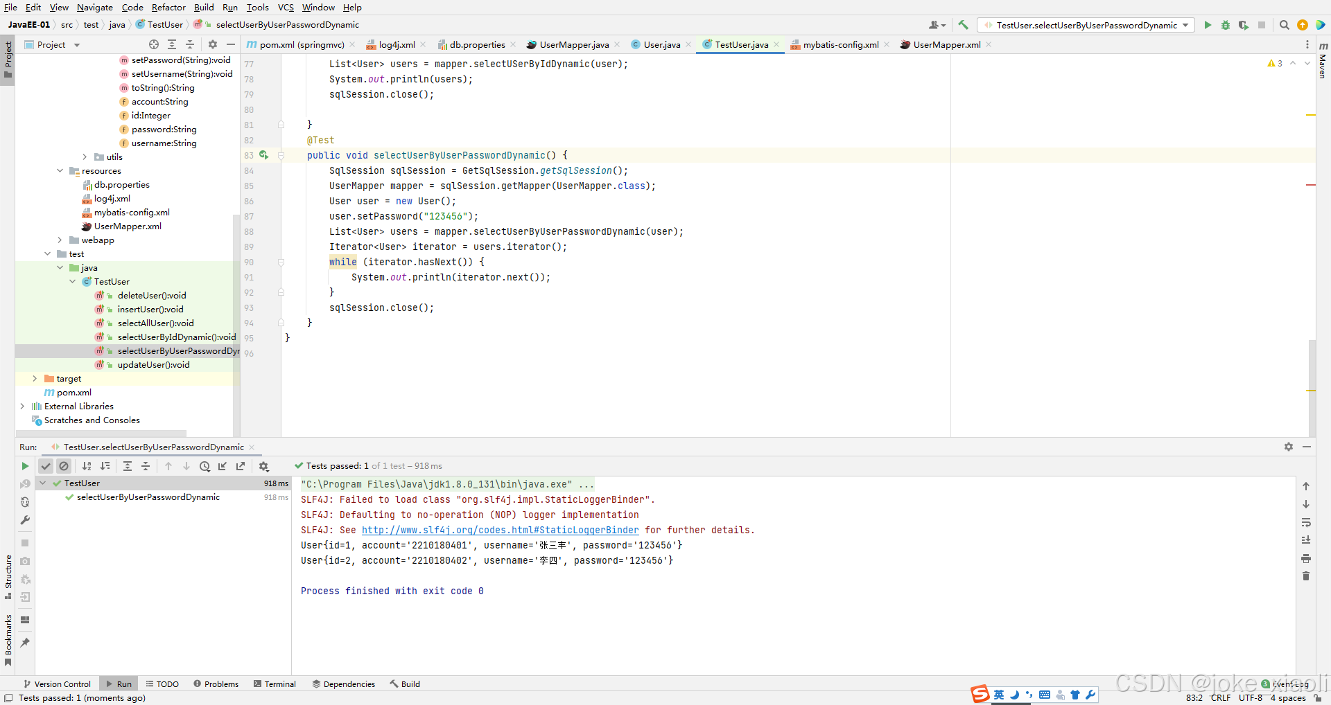
JavaEE-0403学习记录
通过前期准备后,项目已经能够成功运行: 1、在文件UserMapper.java中添加如下代码: List<User> selectUSerByIdDynamic(User user); 2、在文件UserMapper.xml中添加如下代码: <select id"selectUSerByIdDynamic&quo…...
图像处理:使用Numpy和OpenCV实现傅里叶和逆傅里叶变换
文章目录 1、什么是傅里叶变换及其基础理论 1.1 傅里叶变换 1.2 基础理论 2. Numpy 实现傅里叶和逆傅里叶变换 2.1 Numpy 实现傅里叶变换 2.2 实现逆傅里叶变换 2.3 高通滤波示例 3. OpenCV 实现傅里叶变换和逆傅里叶变换及低通滤波示例 3.1 OpenCV 实现傅里叶变换 3.2 实现逆傅…...

洛谷题单2-P5715 【深基3.例8】三位数排序-python-流程图重构
题目描述 给出三个整数 a , b , c ( 0 ≤ a , b , c ≤ 100 ) a,b,c(0\le a,b,c \le 100) a,b,c(0≤a,b,c≤100),要求把这三位整数从小到大排序。 输入格式 输入三个整数 a , b , c a,b,c a,b,c,以空格隔开。 输出格式 输出一行,三个整…...
RNN模型与NLP应用——(7/9)机器翻译与Seq2Seq模型
声明: 本文基于哔站博主【Shusenwang】的视频课程【RNN模型及NLP应用】,结合自身的理解所作,旨在帮助大家了解学习NLP自然语言处理基础知识。配合着视频课程学习效果更佳。 材料来源:【Shusenwang】的视频课程【RNN模型及NLP应用…...

使用YoloV5和Mediapipe实现——上课玩手机检测(附完整源码)
目录 效果展示 应用场景举例 1. 课堂或考试监控(看到这个学生党还会爱我吗) 2. 驾驶安全监控(防止开车玩手机) 3. 企业办公管理(防止工作时间玩手机) 4. 监狱、戒毒所、特殊场所安保 5. 家长监管&am…...