【Python机器学习】实验04(1) 多分类(基于逻辑回归)实践
文章目录
- 多分类以及机器学习实践
- 如何对多个类别进行分类
- 1.1 数据的预处理
- 1.2 训练数据的准备
- 1.3 定义假设函数,代价函数,梯度下降算法(从实验3复制过来)
- 1.4 调用梯度下降算法来学习三个分类模型的参数
- 1.5 利用模型进行预测
- 1.6 评估模型
- 1.7 试试sklearn
- 实验4(1) 请动手完成你们第一个多分类问题,祝好运!完成下面代码
- 2.1 数据读取
- 2.2 训练数据的准备
- 2.3 定义假设函数、代价函数和梯度下降算法
- 2.4 学习这四个分类模型
- 2.5 利用模型进行预测
- 2.6 计算准确率
多分类以及机器学习实践
如何对多个类别进行分类
Iris数据集是常用的分类实验数据集,由Fisher, 1936收集整理。Iris也称鸢尾花卉数据集,是一类多重变量分析的数据集。数据集包含150个数据样本,分为3类,每类50个数据,每个数据包含4个属性。可通过花萼长度,花萼宽度,花瓣长度,花瓣宽度4个属性预测鸢尾花卉属于(Setosa,Versicolour,Virginica)三个种类中的哪一类。
iris以鸢尾花的特征作为数据来源,常用在分类操作中。该数据集由3种不同类型的鸢尾花的各50个样本数据构成。其中的一个种类与另外两个种类是线性可分离的,后两个种类是非线性可分离的。
该数据集包含了4个属性:
Sepal.Length(花萼长度),单位是cm;
Sepal.Width(花萼宽度),单位是cm;
Petal.Length(花瓣长度),单位是cm;
Petal.Width(花瓣宽度),单位是cm;
种类:Iris Setosa(山鸢尾)、Iris Versicolour(杂色鸢尾),以及Iris Virginica(维吉尼亚鸢尾)。
1.1 数据的预处理
import sklearn.datasets as datasets
import pandas as pd
import numpy as np
data=datasets.load_iris()
data
{'data': array([[5.1, 3.5, 1.4, 0.2],[4.9, 3. , 1.4, 0.2],[4.7, 3.2, 1.3, 0.2],[4.6, 3.1, 1.5, 0.2],[5. , 3.6, 1.4, 0.2],[5.4, 3.9, 1.7, 0.4],[4.6, 3.4, 1.4, 0.3],[5. , 3.4, 1.5, 0.2],[4.4, 2.9, 1.4, 0.2],[4.9, 3.1, 1.5, 0.1],[5.4, 3.7, 1.5, 0.2],[4.8, 3.4, 1.6, 0.2],[4.8, 3. , 1.4, 0.1],[4.3, 3. , 1.1, 0.1],[5.8, 4. , 1.2, 0.2],[5.7, 4.4, 1.5, 0.4],[5.4, 3.9, 1.3, 0.4],[5.1, 3.5, 1.4, 0.3],[5.7, 3.8, 1.7, 0.3],[5.1, 3.8, 1.5, 0.3],[5.4, 3.4, 1.7, 0.2],[5.1, 3.7, 1.5, 0.4],[4.6, 3.6, 1. , 0.2],[5.1, 3.3, 1.7, 0.5],[4.8, 3.4, 1.9, 0.2],[5. , 3. , 1.6, 0.2],[5. , 3.4, 1.6, 0.4],[5.2, 3.5, 1.5, 0.2],[5.2, 3.4, 1.4, 0.2],[4.7, 3.2, 1.6, 0.2],[4.8, 3.1, 1.6, 0.2],[5.4, 3.4, 1.5, 0.4],[5.2, 4.1, 1.5, 0.1],[5.5, 4.2, 1.4, 0.2],[4.9, 3.1, 1.5, 0.2],[5. , 3.2, 1.2, 0.2],[5.5, 3.5, 1.3, 0.2],[4.9, 3.6, 1.4, 0.1],[4.4, 3. , 1.3, 0.2],[5.1, 3.4, 1.5, 0.2],[5. , 3.5, 1.3, 0.3],[4.5, 2.3, 1.3, 0.3],[4.4, 3.2, 1.3, 0.2],[5. , 3.5, 1.6, 0.6],[5.1, 3.8, 1.9, 0.4],[4.8, 3. , 1.4, 0.3],[5.1, 3.8, 1.6, 0.2],[4.6, 3.2, 1.4, 0.2],[5.3, 3.7, 1.5, 0.2],[5. , 3.3, 1.4, 0.2],[7. , 3.2, 4.7, 1.4],[6.4, 3.2, 4.5, 1.5],[6.9, 3.1, 4.9, 1.5],[5.5, 2.3, 4. , 1.3],[6.5, 2.8, 4.6, 1.5],[5.7, 2.8, 4.5, 1.3],[6.3, 3.3, 4.7, 1.6],[4.9, 2.4, 3.3, 1. ],[6.6, 2.9, 4.6, 1.3],[5.2, 2.7, 3.9, 1.4],[5. , 2. , 3.5, 1. ],[5.9, 3. , 4.2, 1.5],[6. , 2.2, 4. , 1. ],[6.1, 2.9, 4.7, 1.4],[5.6, 2.9, 3.6, 1.3],[6.7, 3.1, 4.4, 1.4],[5.6, 3. , 4.5, 1.5],[5.8, 2.7, 4.1, 1. ],[6.2, 2.2, 4.5, 1.5],[5.6, 2.5, 3.9, 1.1],[5.9, 3.2, 4.8, 1.8],[6.1, 2.8, 4. , 1.3],[6.3, 2.5, 4.9, 1.5],[6.1, 2.8, 4.7, 1.2],[6.4, 2.9, 4.3, 1.3],[6.6, 3. , 4.4, 1.4],[6.8, 2.8, 4.8, 1.4],[6.7, 3. , 5. , 1.7],[6. , 2.9, 4.5, 1.5],[5.7, 2.6, 3.5, 1. ],[5.5, 2.4, 3.8, 1.1],[5.5, 2.4, 3.7, 1. ],[5.8, 2.7, 3.9, 1.2],[6. , 2.7, 5.1, 1.6],[5.4, 3. , 4.5, 1.5],[6. , 3.4, 4.5, 1.6],[6.7, 3.1, 4.7, 1.5],[6.3, 2.3, 4.4, 1.3],[5.6, 3. , 4.1, 1.3],[5.5, 2.5, 4. , 1.3],[5.5, 2.6, 4.4, 1.2],[6.1, 3. , 4.6, 1.4],[5.8, 2.6, 4. , 1.2],[5. , 2.3, 3.3, 1. ],[5.6, 2.7, 4.2, 1.3],[5.7, 3. , 4.2, 1.2],[5.7, 2.9, 4.2, 1.3],[6.2, 2.9, 4.3, 1.3],[5.1, 2.5, 3. , 1.1],[5.7, 2.8, 4.1, 1.3],[6.3, 3.3, 6. , 2.5],[5.8, 2.7, 5.1, 1.9],[7.1, 3. , 5.9, 2.1],[6.3, 2.9, 5.6, 1.8],[6.5, 3. , 5.8, 2.2],[7.6, 3. , 6.6, 2.1],[4.9, 2.5, 4.5, 1.7],[7.3, 2.9, 6.3, 1.8],[6.7, 2.5, 5.8, 1.8],[7.2, 3.6, 6.1, 2.5],[6.5, 3.2, 5.1, 2. ],[6.4, 2.7, 5.3, 1.9],[6.8, 3. , 5.5, 2.1],[5.7, 2.5, 5. , 2. ],[5.8, 2.8, 5.1, 2.4],[6.4, 3.2, 5.3, 2.3],[6.5, 3. , 5.5, 1.8],[7.7, 3.8, 6.7, 2.2],[7.7, 2.6, 6.9, 2.3],[6. , 2.2, 5. , 1.5],[6.9, 3.2, 5.7, 2.3],[5.6, 2.8, 4.9, 2. ],[7.7, 2.8, 6.7, 2. ],[6.3, 2.7, 4.9, 1.8],[6.7, 3.3, 5.7, 2.1],[7.2, 3.2, 6. , 1.8],[6.2, 2.8, 4.8, 1.8],[6.1, 3. , 4.9, 1.8],[6.4, 2.8, 5.6, 2.1],[7.2, 3. , 5.8, 1.6],[7.4, 2.8, 6.1, 1.9],[7.9, 3.8, 6.4, 2. ],[6.4, 2.8, 5.6, 2.2],[6.3, 2.8, 5.1, 1.5],[6.1, 2.6, 5.6, 1.4],[7.7, 3. , 6.1, 2.3],[6.3, 3.4, 5.6, 2.4],[6.4, 3.1, 5.5, 1.8],[6. , 3. , 4.8, 1.8],[6.9, 3.1, 5.4, 2.1],[6.7, 3.1, 5.6, 2.4],[6.9, 3.1, 5.1, 2.3],[5.8, 2.7, 5.1, 1.9],[6.8, 3.2, 5.9, 2.3],[6.7, 3.3, 5.7, 2.5],[6.7, 3. , 5.2, 2.3],[6.3, 2.5, 5. , 1.9],[6.5, 3. , 5.2, 2. ],[6.2, 3.4, 5.4, 2.3],[5.9, 3. , 5.1, 1.8]]),'target': array([0, 0, 0, 0, 0, 0, 0, 0, 0, 0, 0, 0, 0, 0, 0, 0, 0, 0, 0, 0, 0, 0,0, 0, 0, 0, 0, 0, 0, 0, 0, 0, 0, 0, 0, 0, 0, 0, 0, 0, 0, 0, 0, 0,0, 0, 0, 0, 0, 0, 1, 1, 1, 1, 1, 1, 1, 1, 1, 1, 1, 1, 1, 1, 1, 1,1, 1, 1, 1, 1, 1, 1, 1, 1, 1, 1, 1, 1, 1, 1, 1, 1, 1, 1, 1, 1, 1,1, 1, 1, 1, 1, 1, 1, 1, 1, 1, 1, 1, 2, 2, 2, 2, 2, 2, 2, 2, 2, 2,2, 2, 2, 2, 2, 2, 2, 2, 2, 2, 2, 2, 2, 2, 2, 2, 2, 2, 2, 2, 2, 2,2, 2, 2, 2, 2, 2, 2, 2, 2, 2, 2, 2, 2, 2, 2, 2, 2, 2]),'frame': None,'target_names': array(['setosa', 'versicolor', 'virginica'], dtype='<U10'),'DESCR': '.. _iris_dataset:\n\nIris plants dataset\n--------------------\n\n**Data Set Characteristics:**\n\n :Number of Instances: 150 (50 in each of three classes)\n :Number of Attributes: 4 numeric, predictive attributes and the class\n :Attribute Information:\n - sepal length in cm\n - sepal width in cm\n - petal length in cm\n - petal width in cm\n - class:\n - Iris-Setosa\n - Iris-Versicolour\n - Iris-Virginica\n \n :Summary Statistics:\n\n ============== ==== ==== ======= ===== ====================\n Min Max Mean SD Class Correlation\n ============== ==== ==== ======= ===== ====================\n sepal length: 4.3 7.9 5.84 0.83 0.7826\n sepal width: 2.0 4.4 3.05 0.43 -0.4194\n petal length: 1.0 6.9 3.76 1.76 0.9490 (high!)\n petal width: 0.1 2.5 1.20 0.76 0.9565 (high!)\n ============== ==== ==== ======= ===== ====================\n\n :Missing Attribute Values: None\n :Class Distribution: 33.3% for each of 3 classes.\n :Creator: R.A. Fisher\n :Donor: Michael Marshall (MARSHALL%PLU@io.arc.nasa.gov)\n :Date: July, 1988\n\nThe famous Iris database, first used by Sir R.A. Fisher. The dataset is taken\nfrom Fisher\'s paper. Note that it\'s the same as in R, but not as in the UCI\nMachine Learning Repository, which has two wrong data points.\n\nThis is perhaps the best known database to be found in the\npattern recognition literature. Fisher\'s paper is a classic in the field and\nis referenced frequently to this day. (See Duda & Hart, for example.) The\ndata set contains 3 classes of 50 instances each, where each class refers to a\ntype of iris plant. One class is linearly separable from the other 2; the\nlatter are NOT linearly separable from each other.\n\n.. topic:: References\n\n - Fisher, R.A. "The use of multiple measurements in taxonomic problems"\n Annual Eugenics, 7, Part II, 179-188 (1936); also in "Contributions to\n Mathematical Statistics" (John Wiley, NY, 1950).\n - Duda, R.O., & Hart, P.E. (1973) Pattern Classification and Scene Analysis.\n (Q327.D83) John Wiley & Sons. ISBN 0-471-22361-1. See page 218.\n - Dasarathy, B.V. (1980) "Nosing Around the Neighborhood: A New System\n Structure and Classification Rule for Recognition in Partially Exposed\n Environments". IEEE Transactions on Pattern Analysis and Machine\n Intelligence, Vol. PAMI-2, No. 1, 67-71.\n - Gates, G.W. (1972) "The Reduced Nearest Neighbor Rule". IEEE Transactions\n on Information Theory, May 1972, 431-433.\n - See also: 1988 MLC Proceedings, 54-64. Cheeseman et al"s AUTOCLASS II\n conceptual clustering system finds 3 classes in the data.\n - Many, many more ...','feature_names': ['sepal length (cm)','sepal width (cm)','petal length (cm)','petal width (cm)'],'filename': 'iris.csv','data_module': 'sklearn.datasets.data'}
data_x=data["data"]
data_y=data["target"]
data_x.shape,data_y.shape
((150, 4), (150,))
data_y=data_y.reshape([len(data_y),1])
data_y
array([[0],[0],[0],[0],[0],[0],[0],[0],[0],[0],[0],[0],[0],[0],[0],[0],[0],[0],[0],[0],[0],[0],[0],[0],[0],[0],[0],[0],[0],[0],[0],[0],[0],[0],[0],[0],[0],[0],[0],[0],[0],[0],[0],[0],[0],[0],[0],[0],[0],[0],[1],[1],[1],[1],[1],[1],[1],[1],[1],[1],[1],[1],[1],[1],[1],[1],[1],[1],[1],[1],[1],[1],[1],[1],[1],[1],[1],[1],[1],[1],[1],[1],[1],[1],[1],[1],[1],[1],[1],[1],[1],[1],[1],[1],[1],[1],[1],[1],[1],[1],[2],[2],[2],[2],[2],[2],[2],[2],[2],[2],[2],[2],[2],[2],[2],[2],[2],[2],[2],[2],[2],[2],[2],[2],[2],[2],[2],[2],[2],[2],[2],[2],[2],[2],[2],[2],[2],[2],[2],[2],[2],[2],[2],[2],[2],[2],[2],[2],[2],[2]])
#法1 ,用拼接的方法
data=np.hstack([data_x,data_y])
#法二: 用插入的方法
np.insert(data_x,data_x.shape[1],data_y,axis=1)
array([[5.1, 3.5, 1.4, ..., 2. , 2. , 2. ],[4.9, 3. , 1.4, ..., 2. , 2. , 2. ],[4.7, 3.2, 1.3, ..., 2. , 2. , 2. ],...,[6.5, 3. , 5.2, ..., 2. , 2. , 2. ],[6.2, 3.4, 5.4, ..., 2. , 2. , 2. ],[5.9, 3. , 5.1, ..., 2. , 2. , 2. ]])
data=pd.DataFrame(data,columns=["F1","F2","F3","F4","target"])
data
| F1 | F2 | F3 | F4 | target | |
|---|---|---|---|---|---|
| 0 | 5.1 | 3.5 | 1.4 | 0.2 | 0.0 |
| 1 | 4.9 | 3.0 | 1.4 | 0.2 | 0.0 |
| 2 | 4.7 | 3.2 | 1.3 | 0.2 | 0.0 |
| 3 | 4.6 | 3.1 | 1.5 | 0.2 | 0.0 |
| 4 | 5.0 | 3.6 | 1.4 | 0.2 | 0.0 |
| ... | ... | ... | ... | ... | ... |
| 145 | 6.7 | 3.0 | 5.2 | 2.3 | 2.0 |
| 146 | 6.3 | 2.5 | 5.0 | 1.9 | 2.0 |
| 147 | 6.5 | 3.0 | 5.2 | 2.0 | 2.0 |
| 148 | 6.2 | 3.4 | 5.4 | 2.3 | 2.0 |
| 149 | 5.9 | 3.0 | 5.1 | 1.8 | 2.0 |
150 rows × 5 columns
data.insert(0,"ones",1)
data
| ones | F1 | F2 | F3 | F4 | target | |
|---|---|---|---|---|---|---|
| 0 | 1 | 5.1 | 3.5 | 1.4 | 0.2 | 0.0 |
| 1 | 1 | 4.9 | 3.0 | 1.4 | 0.2 | 0.0 |
| 2 | 1 | 4.7 | 3.2 | 1.3 | 0.2 | 0.0 |
| 3 | 1 | 4.6 | 3.1 | 1.5 | 0.2 | 0.0 |
| 4 | 1 | 5.0 | 3.6 | 1.4 | 0.2 | 0.0 |
| ... | ... | ... | ... | ... | ... | ... |
| 145 | 1 | 6.7 | 3.0 | 5.2 | 2.3 | 2.0 |
| 146 | 1 | 6.3 | 2.5 | 5.0 | 1.9 | 2.0 |
| 147 | 1 | 6.5 | 3.0 | 5.2 | 2.0 | 2.0 |
| 148 | 1 | 6.2 | 3.4 | 5.4 | 2.3 | 2.0 |
| 149 | 1 | 5.9 | 3.0 | 5.1 | 1.8 | 2.0 |
150 rows × 6 columns
data["target"]=data["target"].astype("int32")
data
| ones | F1 | F2 | F3 | F4 | target | |
|---|---|---|---|---|---|---|
| 0 | 1 | 5.1 | 3.5 | 1.4 | 0.2 | 0 |
| 1 | 1 | 4.9 | 3.0 | 1.4 | 0.2 | 0 |
| 2 | 1 | 4.7 | 3.2 | 1.3 | 0.2 | 0 |
| 3 | 1 | 4.6 | 3.1 | 1.5 | 0.2 | 0 |
| 4 | 1 | 5.0 | 3.6 | 1.4 | 0.2 | 0 |
| ... | ... | ... | ... | ... | ... | ... |
| 145 | 1 | 6.7 | 3.0 | 5.2 | 2.3 | 2 |
| 146 | 1 | 6.3 | 2.5 | 5.0 | 1.9 | 2 |
| 147 | 1 | 6.5 | 3.0 | 5.2 | 2.0 | 2 |
| 148 | 1 | 6.2 | 3.4 | 5.4 | 2.3 | 2 |
| 149 | 1 | 5.9 | 3.0 | 5.1 | 1.8 | 2 |
150 rows × 6 columns
1.2 训练数据的准备
data_x
array([[5.1, 3.5, 1.4, 0.2],[4.9, 3. , 1.4, 0.2],[4.7, 3.2, 1.3, 0.2],[4.6, 3.1, 1.5, 0.2],[5. , 3.6, 1.4, 0.2],[5.4, 3.9, 1.7, 0.4],[4.6, 3.4, 1.4, 0.3],[5. , 3.4, 1.5, 0.2],[4.4, 2.9, 1.4, 0.2],[4.9, 3.1, 1.5, 0.1],[5.4, 3.7, 1.5, 0.2],[4.8, 3.4, 1.6, 0.2],[4.8, 3. , 1.4, 0.1],[4.3, 3. , 1.1, 0.1],[5.8, 4. , 1.2, 0.2],[5.7, 4.4, 1.5, 0.4],[5.4, 3.9, 1.3, 0.4],[5.1, 3.5, 1.4, 0.3],[5.7, 3.8, 1.7, 0.3],[5.1, 3.8, 1.5, 0.3],[5.4, 3.4, 1.7, 0.2],[5.1, 3.7, 1.5, 0.4],[4.6, 3.6, 1. , 0.2],[5.1, 3.3, 1.7, 0.5],[4.8, 3.4, 1.9, 0.2],[5. , 3. , 1.6, 0.2],[5. , 3.4, 1.6, 0.4],[5.2, 3.5, 1.5, 0.2],[5.2, 3.4, 1.4, 0.2],[4.7, 3.2, 1.6, 0.2],[4.8, 3.1, 1.6, 0.2],[5.4, 3.4, 1.5, 0.4],[5.2, 4.1, 1.5, 0.1],[5.5, 4.2, 1.4, 0.2],[4.9, 3.1, 1.5, 0.2],[5. , 3.2, 1.2, 0.2],[5.5, 3.5, 1.3, 0.2],[4.9, 3.6, 1.4, 0.1],[4.4, 3. , 1.3, 0.2],[5.1, 3.4, 1.5, 0.2],[5. , 3.5, 1.3, 0.3],[4.5, 2.3, 1.3, 0.3],[4.4, 3.2, 1.3, 0.2],[5. , 3.5, 1.6, 0.6],[5.1, 3.8, 1.9, 0.4],[4.8, 3. , 1.4, 0.3],[5.1, 3.8, 1.6, 0.2],[4.6, 3.2, 1.4, 0.2],[5.3, 3.7, 1.5, 0.2],[5. , 3.3, 1.4, 0.2],[7. , 3.2, 4.7, 1.4],[6.4, 3.2, 4.5, 1.5],[6.9, 3.1, 4.9, 1.5],[5.5, 2.3, 4. , 1.3],[6.5, 2.8, 4.6, 1.5],[5.7, 2.8, 4.5, 1.3],[6.3, 3.3, 4.7, 1.6],[4.9, 2.4, 3.3, 1. ],[6.6, 2.9, 4.6, 1.3],[5.2, 2.7, 3.9, 1.4],[5. , 2. , 3.5, 1. ],[5.9, 3. , 4.2, 1.5],[6. , 2.2, 4. , 1. ],[6.1, 2.9, 4.7, 1.4],[5.6, 2.9, 3.6, 1.3],[6.7, 3.1, 4.4, 1.4],[5.6, 3. , 4.5, 1.5],[5.8, 2.7, 4.1, 1. ],[6.2, 2.2, 4.5, 1.5],[5.6, 2.5, 3.9, 1.1],[5.9, 3.2, 4.8, 1.8],[6.1, 2.8, 4. , 1.3],[6.3, 2.5, 4.9, 1.5],[6.1, 2.8, 4.7, 1.2],[6.4, 2.9, 4.3, 1.3],[6.6, 3. , 4.4, 1.4],[6.8, 2.8, 4.8, 1.4],[6.7, 3. , 5. , 1.7],[6. , 2.9, 4.5, 1.5],[5.7, 2.6, 3.5, 1. ],[5.5, 2.4, 3.8, 1.1],[5.5, 2.4, 3.7, 1. ],[5.8, 2.7, 3.9, 1.2],[6. , 2.7, 5.1, 1.6],[5.4, 3. , 4.5, 1.5],[6. , 3.4, 4.5, 1.6],[6.7, 3.1, 4.7, 1.5],[6.3, 2.3, 4.4, 1.3],[5.6, 3. , 4.1, 1.3],[5.5, 2.5, 4. , 1.3],[5.5, 2.6, 4.4, 1.2],[6.1, 3. , 4.6, 1.4],[5.8, 2.6, 4. , 1.2],[5. , 2.3, 3.3, 1. ],[5.6, 2.7, 4.2, 1.3],[5.7, 3. , 4.2, 1.2],[5.7, 2.9, 4.2, 1.3],[6.2, 2.9, 4.3, 1.3],[5.1, 2.5, 3. , 1.1],[5.7, 2.8, 4.1, 1.3],[6.3, 3.3, 6. , 2.5],[5.8, 2.7, 5.1, 1.9],[7.1, 3. , 5.9, 2.1],[6.3, 2.9, 5.6, 1.8],[6.5, 3. , 5.8, 2.2],[7.6, 3. , 6.6, 2.1],[4.9, 2.5, 4.5, 1.7],[7.3, 2.9, 6.3, 1.8],[6.7, 2.5, 5.8, 1.8],[7.2, 3.6, 6.1, 2.5],[6.5, 3.2, 5.1, 2. ],[6.4, 2.7, 5.3, 1.9],[6.8, 3. , 5.5, 2.1],[5.7, 2.5, 5. , 2. ],[5.8, 2.8, 5.1, 2.4],[6.4, 3.2, 5.3, 2.3],[6.5, 3. , 5.5, 1.8],[7.7, 3.8, 6.7, 2.2],[7.7, 2.6, 6.9, 2.3],[6. , 2.2, 5. , 1.5],[6.9, 3.2, 5.7, 2.3],[5.6, 2.8, 4.9, 2. ],[7.7, 2.8, 6.7, 2. ],[6.3, 2.7, 4.9, 1.8],[6.7, 3.3, 5.7, 2.1],[7.2, 3.2, 6. , 1.8],[6.2, 2.8, 4.8, 1.8],[6.1, 3. , 4.9, 1.8],[6.4, 2.8, 5.6, 2.1],[7.2, 3. , 5.8, 1.6],[7.4, 2.8, 6.1, 1.9],[7.9, 3.8, 6.4, 2. ],[6.4, 2.8, 5.6, 2.2],[6.3, 2.8, 5.1, 1.5],[6.1, 2.6, 5.6, 1.4],[7.7, 3. , 6.1, 2.3],[6.3, 3.4, 5.6, 2.4],[6.4, 3.1, 5.5, 1.8],[6. , 3. , 4.8, 1.8],[6.9, 3.1, 5.4, 2.1],[6.7, 3.1, 5.6, 2.4],[6.9, 3.1, 5.1, 2.3],[5.8, 2.7, 5.1, 1.9],[6.8, 3.2, 5.9, 2.3],[6.7, 3.3, 5.7, 2.5],[6.7, 3. , 5.2, 2.3],[6.3, 2.5, 5. , 1.9],[6.5, 3. , 5.2, 2. ],[6.2, 3.4, 5.4, 2.3],[5.9, 3. , 5.1, 1.8]])
data_x=np.insert(data_x,0,1,axis=1)
data_x.shape,data_y.shape
((150, 5), (150, 1))
#训练数据的特征和标签
data_x,data_y
(array([[1. , 5.1, 3.5, 1.4, 0.2],[1. , 4.9, 3. , 1.4, 0.2],[1. , 4.7, 3.2, 1.3, 0.2],[1. , 4.6, 3.1, 1.5, 0.2],[1. , 5. , 3.6, 1.4, 0.2],[1. , 5.4, 3.9, 1.7, 0.4],[1. , 4.6, 3.4, 1.4, 0.3],[1. , 5. , 3.4, 1.5, 0.2],[1. , 4.4, 2.9, 1.4, 0.2],[1. , 4.9, 3.1, 1.5, 0.1],[1. , 5.4, 3.7, 1.5, 0.2],[1. , 4.8, 3.4, 1.6, 0.2],[1. , 4.8, 3. , 1.4, 0.1],[1. , 4.3, 3. , 1.1, 0.1],[1. , 5.8, 4. , 1.2, 0.2],[1. , 5.7, 4.4, 1.5, 0.4],[1. , 5.4, 3.9, 1.3, 0.4],[1. , 5.1, 3.5, 1.4, 0.3],[1. , 5.7, 3.8, 1.7, 0.3],[1. , 5.1, 3.8, 1.5, 0.3],[1. , 5.4, 3.4, 1.7, 0.2],[1. , 5.1, 3.7, 1.5, 0.4],[1. , 4.6, 3.6, 1. , 0.2],[1. , 5.1, 3.3, 1.7, 0.5],[1. , 4.8, 3.4, 1.9, 0.2],[1. , 5. , 3. , 1.6, 0.2],[1. , 5. , 3.4, 1.6, 0.4],[1. , 5.2, 3.5, 1.5, 0.2],[1. , 5.2, 3.4, 1.4, 0.2],[1. , 4.7, 3.2, 1.6, 0.2],[1. , 4.8, 3.1, 1.6, 0.2],[1. , 5.4, 3.4, 1.5, 0.4],[1. , 5.2, 4.1, 1.5, 0.1],[1. , 5.5, 4.2, 1.4, 0.2],[1. , 4.9, 3.1, 1.5, 0.2],[1. , 5. , 3.2, 1.2, 0.2],[1. , 5.5, 3.5, 1.3, 0.2],[1. , 4.9, 3.6, 1.4, 0.1],[1. , 4.4, 3. , 1.3, 0.2],[1. , 5.1, 3.4, 1.5, 0.2],[1. , 5. , 3.5, 1.3, 0.3],[1. , 4.5, 2.3, 1.3, 0.3],[1. , 4.4, 3.2, 1.3, 0.2],[1. , 5. , 3.5, 1.6, 0.6],[1. , 5.1, 3.8, 1.9, 0.4],[1. , 4.8, 3. , 1.4, 0.3],[1. , 5.1, 3.8, 1.6, 0.2],[1. , 4.6, 3.2, 1.4, 0.2],[1. , 5.3, 3.7, 1.5, 0.2],[1. , 5. , 3.3, 1.4, 0.2],[1. , 7. , 3.2, 4.7, 1.4],[1. , 6.4, 3.2, 4.5, 1.5],[1. , 6.9, 3.1, 4.9, 1.5],[1. , 5.5, 2.3, 4. , 1.3],[1. , 6.5, 2.8, 4.6, 1.5],[1. , 5.7, 2.8, 4.5, 1.3],[1. , 6.3, 3.3, 4.7, 1.6],[1. , 4.9, 2.4, 3.3, 1. ],[1. , 6.6, 2.9, 4.6, 1.3],[1. , 5.2, 2.7, 3.9, 1.4],[1. , 5. , 2. , 3.5, 1. ],[1. , 5.9, 3. , 4.2, 1.5],[1. , 6. , 2.2, 4. , 1. ],[1. , 6.1, 2.9, 4.7, 1.4],[1. , 5.6, 2.9, 3.6, 1.3],[1. , 6.7, 3.1, 4.4, 1.4],[1. , 5.6, 3. , 4.5, 1.5],[1. , 5.8, 2.7, 4.1, 1. ],[1. , 6.2, 2.2, 4.5, 1.5],[1. , 5.6, 2.5, 3.9, 1.1],[1. , 5.9, 3.2, 4.8, 1.8],[1. , 6.1, 2.8, 4. , 1.3],[1. , 6.3, 2.5, 4.9, 1.5],[1. , 6.1, 2.8, 4.7, 1.2],[1. , 6.4, 2.9, 4.3, 1.3],[1. , 6.6, 3. , 4.4, 1.4],[1. , 6.8, 2.8, 4.8, 1.4],[1. , 6.7, 3. , 5. , 1.7],[1. , 6. , 2.9, 4.5, 1.5],[1. , 5.7, 2.6, 3.5, 1. ],[1. , 5.5, 2.4, 3.8, 1.1],[1. , 5.5, 2.4, 3.7, 1. ],[1. , 5.8, 2.7, 3.9, 1.2],[1. , 6. , 2.7, 5.1, 1.6],[1. , 5.4, 3. , 4.5, 1.5],[1. , 6. , 3.4, 4.5, 1.6],[1. , 6.7, 3.1, 4.7, 1.5],[1. , 6.3, 2.3, 4.4, 1.3],[1. , 5.6, 3. , 4.1, 1.3],[1. , 5.5, 2.5, 4. , 1.3],[1. , 5.5, 2.6, 4.4, 1.2],[1. , 6.1, 3. , 4.6, 1.4],[1. , 5.8, 2.6, 4. , 1.2],[1. , 5. , 2.3, 3.3, 1. ],[1. , 5.6, 2.7, 4.2, 1.3],[1. , 5.7, 3. , 4.2, 1.2],[1. , 5.7, 2.9, 4.2, 1.3],[1. , 6.2, 2.9, 4.3, 1.3],[1. , 5.1, 2.5, 3. , 1.1],[1. , 5.7, 2.8, 4.1, 1.3],[1. , 6.3, 3.3, 6. , 2.5],[1. , 5.8, 2.7, 5.1, 1.9],[1. , 7.1, 3. , 5.9, 2.1],[1. , 6.3, 2.9, 5.6, 1.8],[1. , 6.5, 3. , 5.8, 2.2],[1. , 7.6, 3. , 6.6, 2.1],[1. , 4.9, 2.5, 4.5, 1.7],[1. , 7.3, 2.9, 6.3, 1.8],[1. , 6.7, 2.5, 5.8, 1.8],[1. , 7.2, 3.6, 6.1, 2.5],[1. , 6.5, 3.2, 5.1, 2. ],[1. , 6.4, 2.7, 5.3, 1.9],[1. , 6.8, 3. , 5.5, 2.1],[1. , 5.7, 2.5, 5. , 2. ],[1. , 5.8, 2.8, 5.1, 2.4],[1. , 6.4, 3.2, 5.3, 2.3],[1. , 6.5, 3. , 5.5, 1.8],[1. , 7.7, 3.8, 6.7, 2.2],[1. , 7.7, 2.6, 6.9, 2.3],[1. , 6. , 2.2, 5. , 1.5],[1. , 6.9, 3.2, 5.7, 2.3],[1. , 5.6, 2.8, 4.9, 2. ],[1. , 7.7, 2.8, 6.7, 2. ],[1. , 6.3, 2.7, 4.9, 1.8],[1. , 6.7, 3.3, 5.7, 2.1],[1. , 7.2, 3.2, 6. , 1.8],[1. , 6.2, 2.8, 4.8, 1.8],[1. , 6.1, 3. , 4.9, 1.8],[1. , 6.4, 2.8, 5.6, 2.1],[1. , 7.2, 3. , 5.8, 1.6],[1. , 7.4, 2.8, 6.1, 1.9],[1. , 7.9, 3.8, 6.4, 2. ],[1. , 6.4, 2.8, 5.6, 2.2],[1. , 6.3, 2.8, 5.1, 1.5],[1. , 6.1, 2.6, 5.6, 1.4],[1. , 7.7, 3. , 6.1, 2.3],[1. , 6.3, 3.4, 5.6, 2.4],[1. , 6.4, 3.1, 5.5, 1.8],[1. , 6. , 3. , 4.8, 1.8],[1. , 6.9, 3.1, 5.4, 2.1],[1. , 6.7, 3.1, 5.6, 2.4],[1. , 6.9, 3.1, 5.1, 2.3],[1. , 5.8, 2.7, 5.1, 1.9],[1. , 6.8, 3.2, 5.9, 2.3],[1. , 6.7, 3.3, 5.7, 2.5],[1. , 6.7, 3. , 5.2, 2.3],[1. , 6.3, 2.5, 5. , 1.9],[1. , 6.5, 3. , 5.2, 2. ],[1. , 6.2, 3.4, 5.4, 2.3],[1. , 5.9, 3. , 5.1, 1.8]]),array([[0],[0],[0],[0],[0],[0],[0],[0],[0],[0],[0],[0],[0],[0],[0],[0],[0],[0],[0],[0],[0],[0],[0],[0],[0],[0],[0],[0],[0],[0],[0],[0],[0],[0],[0],[0],[0],[0],[0],[0],[0],[0],[0],[0],[0],[0],[0],[0],[0],[0],[1],[1],[1],[1],[1],[1],[1],[1],[1],[1],[1],[1],[1],[1],[1],[1],[1],[1],[1],[1],[1],[1],[1],[1],[1],[1],[1],[1],[1],[1],[1],[1],[1],[1],[1],[1],[1],[1],[1],[1],[1],[1],[1],[1],[1],[1],[1],[1],[1],[1],[2],[2],[2],[2],[2],[2],[2],[2],[2],[2],[2],[2],[2],[2],[2],[2],[2],[2],[2],[2],[2],[2],[2],[2],[2],[2],[2],[2],[2],[2],[2],[2],[2],[2],[2],[2],[2],[2],[2],[2],[2],[2],[2],[2],[2],[2],[2],[2],[2],[2]]))
由于有三个类别,那么在训练时三类数据要分开
data1=data.copy()
data1
| ones | F1 | F2 | F3 | F4 | target | |
|---|---|---|---|---|---|---|
| 0 | 1 | 5.1 | 3.5 | 1.4 | 0.2 | 0 |
| 1 | 1 | 4.9 | 3.0 | 1.4 | 0.2 | 0 |
| 2 | 1 | 4.7 | 3.2 | 1.3 | 0.2 | 0 |
| 3 | 1 | 4.6 | 3.1 | 1.5 | 0.2 | 0 |
| 4 | 1 | 5.0 | 3.6 | 1.4 | 0.2 | 0 |
| ... | ... | ... | ... | ... | ... | ... |
| 145 | 1 | 6.7 | 3.0 | 5.2 | 2.3 | 2 |
| 146 | 1 | 6.3 | 2.5 | 5.0 | 1.9 | 2 |
| 147 | 1 | 6.5 | 3.0 | 5.2 | 2.0 | 2 |
| 148 | 1 | 6.2 | 3.4 | 5.4 | 2.3 | 2 |
| 149 | 1 | 5.9 | 3.0 | 5.1 | 1.8 | 2 |
150 rows × 6 columns
data
data1.loc[data["target"]!=0,"target"]=0
data1.loc[data["target"]==0,"target"]=1
data1
| ones | F1 | F2 | F3 | F4 | target | |
|---|---|---|---|---|---|---|
| 0 | 1 | 5.1 | 3.5 | 1.4 | 0.2 | 1 |
| 1 | 1 | 4.9 | 3.0 | 1.4 | 0.2 | 1 |
| 2 | 1 | 4.7 | 3.2 | 1.3 | 0.2 | 1 |
| 3 | 1 | 4.6 | 3.1 | 1.5 | 0.2 | 1 |
| 4 | 1 | 5.0 | 3.6 | 1.4 | 0.2 | 1 |
| ... | ... | ... | ... | ... | ... | ... |
| 145 | 1 | 6.7 | 3.0 | 5.2 | 2.3 | 0 |
| 146 | 1 | 6.3 | 2.5 | 5.0 | 1.9 | 0 |
| 147 | 1 | 6.5 | 3.0 | 5.2 | 2.0 | 0 |
| 148 | 1 | 6.2 | 3.4 | 5.4 | 2.3 | 0 |
| 149 | 1 | 5.9 | 3.0 | 5.1 | 1.8 | 0 |
150 rows × 6 columns
data1_x=data1.iloc[:,:data1.shape[1]-1].values
data1_y=data1.iloc[:,data1.shape[1]-1].values
data1_x.shape,data1_y.shape
((150, 5), (150,))
#针对第二类,即第二个分类器的数据
data2=data.copy()
data2.loc[data["target"]==1,"target"]=1
data2.loc[data["target"]!=1,"target"]=0
data2["target"]==0
0      True
1      True
2      True
3      True
4      True...
145    True
146    True
147    True
148    True
149    True
Name: target, Length: 150, dtype: bool
data2.shape[1]
6
data2.iloc[50:55,:]
| ones | F1 | F2 | F3 | F4 | target | |
|---|---|---|---|---|---|---|
| 50 | 1 | 7.0 | 3.2 | 4.7 | 1.4 | 1 |
| 51 | 1 | 6.4 | 3.2 | 4.5 | 1.5 | 1 |
| 52 | 1 | 6.9 | 3.1 | 4.9 | 1.5 | 1 |
| 53 | 1 | 5.5 | 2.3 | 4.0 | 1.3 | 1 |
| 54 | 1 | 6.5 | 2.8 | 4.6 | 1.5 | 1 |
data2_x=data2.iloc[:,:data2.shape[1]-1].values
data2_y=data2.iloc[:,data2.shape[1]-1].values
#针对第三类,即第三个分类器的数据
data3=data.copy()
data3.loc[data["target"]==2,"target"]=1
data3.loc[data["target"]!=2,"target"]=0
data3
| ones | F1 | F2 | F3 | F4 | target | |
|---|---|---|---|---|---|---|
| 0 | 1 | 5.1 | 3.5 | 1.4 | 0.2 | 0 |
| 1 | 1 | 4.9 | 3.0 | 1.4 | 0.2 | 0 |
| 2 | 1 | 4.7 | 3.2 | 1.3 | 0.2 | 0 |
| 3 | 1 | 4.6 | 3.1 | 1.5 | 0.2 | 0 |
| 4 | 1 | 5.0 | 3.6 | 1.4 | 0.2 | 0 |
| ... | ... | ... | ... | ... | ... | ... |
| 145 | 1 | 6.7 | 3.0 | 5.2 | 2.3 | 1 |
| 146 | 1 | 6.3 | 2.5 | 5.0 | 1.9 | 1 |
| 147 | 1 | 6.5 | 3.0 | 5.2 | 2.0 | 1 |
| 148 | 1 | 6.2 | 3.4 | 5.4 | 2.3 | 1 |
| 149 | 1 | 5.9 | 3.0 | 5.1 | 1.8 | 1 |
150 rows × 6 columns
data3_x=data3.iloc[:,:data3.shape[1]-1].values
data3_y=data3.iloc[:,data3.shape[1]-1].values
1.3 定义假设函数,代价函数,梯度下降算法(从实验3复制过来)
def sigmoid(z):return 1 / (1 + np.exp(-z))
def h(X,w):z=X@wh=sigmoid(z)return h
#代价函数构造
def cost(X,w,y):#当X(m,n+1),y(m,),w(n+1,1)y_hat=sigmoid(X@w)right=np.multiply(y.ravel(),np.log(y_hat).ravel())+np.multiply((1-y).ravel(),np.log(1-y_hat).ravel())cost=-np.sum(right)/X.shape[0]return cost
def sigmoid(z):return 1 / (1 + np.exp(-z))def h(X,w):z=X@wh=sigmoid(z)return h#代价函数构造
def cost(X,w,y):#当X(m,n+1),y(m,),w(n+1,1)y_hat=sigmoid(X@w)right=np.multiply(y.ravel(),np.log(y_hat).ravel())+np.multiply((1-y).ravel(),np.log(1-y_hat).ravel())cost=-np.sum(right)/X.shape[0]return costdef grandient(X,y,iter_num,alpha):y=y.reshape((X.shape[0],1))w=np.zeros((X.shape[1],1))cost_lst=[]  for i in range(iter_num):y_pred=h(X,w)-ytemp=np.zeros((X.shape[1],1))for j in range(X.shape[1]):right=np.multiply(y_pred.ravel(),X[:,j])gradient=1/(X.shape[0])*(np.sum(right))temp[j,0]=w[j,0]-alpha*gradientw=tempcost_lst.append(cost(X,w,y.ravel()))return w,cost_lst
1.4 调用梯度下降算法来学习三个分类模型的参数
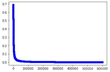
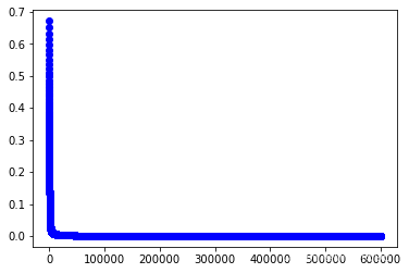
#初始化超参数
iter_num,alpha=600000,0.001
#训练第一个模型
w1,cost_lst1=grandient(data1_x,data1_y,iter_num,alpha)
import matplotlib.pyplot as plt
plt.plot(range(iter_num),cost_lst1,"b-o")
[<matplotlib.lines.Line2D at 0x2562630b100>]
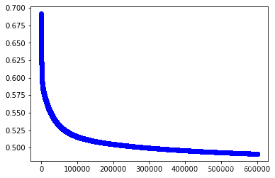
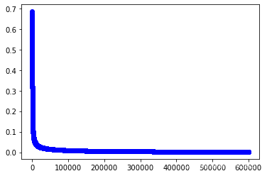
#训练第二个模型
w2,cost_lst2=grandient(data2_x,data2_y,iter_num,alpha)
import matplotlib.pyplot as plt
plt.plot(range(iter_num),cost_lst2,"b-o")
[<matplotlib.lines.Line2D at 0x25628114280>]
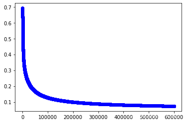
#训练第三个模型
w3,cost_lst3=grandient(data3_x,data3_y,iter_num,alpha)
w3
array([[-3.22437049],[-3.50214058],[-3.50286355],[ 5.16580317],[ 5.89898368]])
import matplotlib.pyplot as plt
plt.plot(range(iter_num),cost_lst3,"b-o")
[<matplotlib.lines.Line2D at 0x2562e0f81c0>]
1.5 利用模型进行预测
h(data_x,w3)
array([[1.48445441e-11],[1.72343968e-10],[1.02798153e-10],[5.81975546e-10],[1.48434710e-11],[1.95971176e-11],[2.18959639e-10],[5.01346874e-11],[1.40930075e-09],[1.12830635e-10],[4.31888744e-12],[1.69308343e-10],[1.35613372e-10],[1.65858883e-10],[7.89880725e-14],[4.23224675e-13],[2.48199140e-12],[2.67766642e-11],[5.39314286e-12],[1.56935848e-11],[3.47096426e-11],[4.01827075e-11],[7.63005509e-12],[8.26864773e-10],[7.97484594e-10],[3.41189783e-10],[2.73442178e-10],[1.75314894e-11],[1.48456174e-11],[4.84204982e-10],[4.84239990e-10],[4.01914238e-11],[1.18813180e-12],[3.14985611e-13],[2.03524473e-10],[2.14461446e-11],[2.18189955e-12],[1.16799745e-11],[5.92281641e-10],[3.53217554e-11],[2.26727669e-11],[8.74004884e-09],[2.93949962e-10],[6.26783110e-10],[2.23513465e-10],[4.41246960e-10],[1.45841303e-11],[2.44584721e-10],[6.13010507e-12],[4.24539165e-11],[1.64123143e-03],[8.55503211e-03],[1.65105645e-02],[9.87814122e-02],[3.97290777e-02],[1.11076040e-01],[4.19003715e-02],[2.88426221e-03],[6.27161978e-03],[7.67020481e-02],[2.27204861e-02],[2.08212169e-02],[4.58067633e-03],[9.90450665e-02],[1.19419048e-03],[1.41462060e-03],[2.22638069e-01],[2.68940904e-03],[3.66014737e-01],[6.97791873e-03],[5.78803255e-01],[2.32071970e-03],[5.28941621e-01],[4.57649874e-02],[2.69208900e-03],[2.84603646e-03],[2.20421076e-02],[2.07507605e-01],[9.10460936e-02],[2.44824946e-04],[8.37509821e-03],[2.78543808e-03],[3.11283202e-03],[8.89831833e-01],[3.65880536e-01],[3.03993844e-02],[1.18930239e-02],[4.99150151e-02],[1.10252946e-02],[5.15923462e-02],[1.43653056e-01],[4.41610209e-02],[7.37513950e-03],[2.88447014e-03],[5.07366744e-02],[7.24617687e-03],[1.83460602e-02],[5.40874928e-03],[3.87210511e-04],[1.55791816e-02],[9.99862942e-01],[9.89637526e-01],[9.86183040e-01],[9.83705644e-01],[9.98410187e-01],[9.97834502e-01],[9.84208537e-01],[9.85434538e-01],[9.94141336e-01],[9.94561329e-01],[7.20333384e-01],[9.70431293e-01],[9.62754456e-01],[9.96609064e-01],[9.99222270e-01],[9.83684437e-01],[9.26437633e-01],[9.83486260e-01],[9.99950496e-01],[9.39002061e-01],[9.88043323e-01],[9.88637702e-01],[9.98357641e-01],[7.65848930e-01],[9.73006160e-01],[8.76969899e-01],[6.61137141e-01],[6.97324053e-01],[9.97185846e-01],[6.11033594e-01],[9.77494647e-01],[6.58573810e-01],[9.98437920e-01],[5.24529693e-01],[9.70465066e-01],[9.87624920e-01],[9.97236435e-01],[9.26432706e-01],[6.61104746e-01],[8.84442100e-01],[9.96082862e-01],[8.40940308e-01],[9.89637526e-01],[9.96974990e-01],[9.97386310e-01],[9.62040470e-01],[9.52214579e-01],[8.96902215e-01],[9.90200940e-01],[9.28785160e-01]])
#将数据输入三个模型的看看结果
multi_pred=pd.DataFrame(zip(h(data_x,w1).ravel(),h(data_x,w2).ravel(),h(data_x,w3).ravel()))
multi_pred
| 0 | 1 | 2 | |
|---|---|---|---|
| 0 | 0.999297 | 0.108037 | 1.484454e-11 |
| 1 | 0.997061 | 0.270814 | 1.723440e-10 |
| 2 | 0.998633 | 0.164710 | 1.027982e-10 |
| 3 | 0.995774 | 0.231910 | 5.819755e-10 |
| 4 | 0.999415 | 0.085259 | 1.484347e-11 |
| ... | ... | ... | ... |
| 145 | 0.000007 | 0.127574 | 9.620405e-01 |
| 146 | 0.000006 | 0.496389 | 9.522146e-01 |
| 147 | 0.000010 | 0.234745 | 8.969022e-01 |
| 148 | 0.000006 | 0.058444 | 9.902009e-01 |
| 149 | 0.000014 | 0.284295 | 9.287852e-01 |
150 rows × 3 columns
multi_pred.values[:3]
array([[9.99297209e-01, 1.08037473e-01, 1.48445441e-11],[9.97060801e-01, 2.70813780e-01, 1.72343968e-10],[9.98632728e-01, 1.64709623e-01, 1.02798153e-10]])
#每个样本的预测值
np.argmax(multi_pred.values,axis=1)
array([0, 0, 0, 0, 0, 0, 0, 0, 0, 0, 0, 0, 0, 0, 0, 0, 0, 0, 0, 0, 0, 0,0, 0, 0, 0, 0, 0, 0, 0, 0, 0, 0, 0, 0, 0, 0, 0, 0, 0, 0, 0, 0, 0,0, 0, 0, 0, 0, 0, 1, 1, 1, 1, 1, 1, 1, 1, 1, 1, 1, 1, 1, 1, 1, 1,1, 1, 1, 1, 2, 1, 1, 1, 1, 1, 1, 1, 1, 1, 1, 1, 1, 2, 2, 1, 1, 1,1, 1, 1, 1, 1, 1, 1, 1, 1, 1, 1, 1, 2, 2, 2, 2, 2, 2, 2, 2, 2, 2,2, 2, 2, 2, 2, 2, 2, 2, 2, 2, 2, 2, 2, 2, 2, 2, 2, 2, 2, 1, 2, 2,2, 1, 2, 2, 2, 2, 2, 2, 2, 2, 2, 2, 2, 2, 2, 2, 2, 2], dtype=int64)
#每个样本的真实值
data_y
array([[0],[0],[0],[0],[0],[0],[0],[0],[0],[0],[0],[0],[0],[0],[0],[0],[0],[0],[0],[0],[0],[0],[0],[0],[0],[0],[0],[0],[0],[0],[0],[0],[0],[0],[0],[0],[0],[0],[0],[0],[0],[0],[0],[0],[0],[0],[0],[0],[0],[0],[1],[1],[1],[1],[1],[1],[1],[1],[1],[1],[1],[1],[1],[1],[1],[1],[1],[1],[1],[1],[1],[1],[1],[1],[1],[1],[1],[1],[1],[1],[1],[1],[1],[1],[1],[1],[1],[1],[1],[1],[1],[1],[1],[1],[1],[1],[1],[1],[1],[1],[2],[2],[2],[2],[2],[2],[2],[2],[2],[2],[2],[2],[2],[2],[2],[2],[2],[2],[2],[2],[2],[2],[2],[2],[2],[2],[2],[2],[2],[2],[2],[2],[2],[2],[2],[2],[2],[2],[2],[2],[2],[2],[2],[2],[2],[2],[2],[2],[2],[2]])
1.6 评估模型
np.argmax(multi_pred.values,axis=1)==data_y.ravel()
array([ True, True, True, True, True, True, True, True, True,True, True, True, True, True, True, True, True, True,True, True, True, True, True, True, True, True, True,True, True, True, True, True, True, True, True, True,True, True, True, True, True, True, True, True, True,True, True, True, True, True, True, True, True, True,True, True, True, True, True, True, True, True, True,True, True, True, True, True, True, True, False, True,True, True, True, True, True, True, True, True, True,True, True, False, False, True, True, True, True, True,True, True, True, True, True, True, True, True, True,True, True, True, True, True, True, True, True, True,True, True, True, True, True, True, True, True, True,True, True, True, True, True, True, True, True, True,True, True, True, False, True, True, True, False, True,True, True, True, True, True, True, True, True, True,True, True, True, True, True, True])
np.sum(np.argmax(multi_pred.values,axis=1)==data_y.ravel())
145
np.sum(np.argmax(multi_pred.values,axis=1)==data_y.ravel())/len(data)
0.9666666666666667
1.7 试试sklearn
from sklearn.linear_model import LogisticRegression
#建立第一个模型
clf1=LogisticRegression()
clf1.fit(data1_x,data1_y)
#建立第二个模型
clf2=LogisticRegression()
clf2.fit(data2_x,data2_y)
#建立第三个模型
clf3=LogisticRegression()
clf3.fit(data3_x,data3_y)
LogisticRegression()
y_pred1=clf1.predict(data_x)
y_pred2=clf2.predict(data_x)
y_pred3=clf3.predict(data_x)
#可视化各模型的预测结果
multi_pred=pd.DataFrame(zip(y_pred1,y_pred2,y_pred3),columns=["模型1","模糊2","模型3"])
multi_pred
| 模型1 | 模糊2 | 模型3 | |
|---|---|---|---|
| 0 | 1 | 0 | 0 |
| 1 | 1 | 0 | 0 |
| 2 | 1 | 0 | 0 |
| 3 | 1 | 0 | 0 |
| 4 | 1 | 0 | 0 |
| ... | ... | ... | ... |
| 145 | 0 | 0 | 1 |
| 146 | 0 | 1 | 1 |
| 147 | 0 | 0 | 1 |
| 148 | 0 | 0 | 1 |
| 149 | 0 | 0 | 1 |
150 rows × 3 columns
#判断预测结果
np.argmax(multi_pred.values,axis=1)
array([0, 0, 0, 0, 0, 0, 0, 0, 0, 0, 0, 0, 0, 0, 0, 0, 0, 0, 0, 0, 0, 0,0, 0, 0, 0, 0, 0, 0, 0, 0, 0, 0, 0, 0, 0, 0, 0, 0, 0, 0, 0, 0, 0,0, 0, 0, 0, 0, 0, 0, 0, 0, 1, 0, 1, 0, 1, 0, 0, 1, 0, 1, 0, 0, 0,0, 1, 1, 1, 2, 0, 1, 1, 0, 0, 0, 2, 0, 1, 1, 1, 0, 1, 0, 0, 0, 1,0, 1, 1, 0, 1, 1, 1, 0, 0, 0, 1, 0, 2, 2, 2, 2, 2, 2, 1, 1, 1, 2,2, 2, 2, 1, 2, 2, 2, 2, 1, 1, 2, 2, 1, 2, 2, 2, 2, 2, 2, 2, 1, 2,2, 1, 1, 2, 2, 2, 2, 2, 2, 2, 2, 2, 2, 2, 1, 2, 2, 2], dtype=int64)
data_y.ravel()
array([0, 0, 0, 0, 0, 0, 0, 0, 0, 0, 0, 0, 0, 0, 0, 0, 0, 0, 0, 0, 0, 0,0, 0, 0, 0, 0, 0, 0, 0, 0, 0, 0, 0, 0, 0, 0, 0, 0, 0, 0, 0, 0, 0,0, 0, 0, 0, 0, 0, 1, 1, 1, 1, 1, 1, 1, 1, 1, 1, 1, 1, 1, 1, 1, 1,1, 1, 1, 1, 1, 1, 1, 1, 1, 1, 1, 1, 1, 1, 1, 1, 1, 1, 1, 1, 1, 1,1, 1, 1, 1, 1, 1, 1, 1, 1, 1, 1, 1, 2, 2, 2, 2, 2, 2, 2, 2, 2, 2,2, 2, 2, 2, 2, 2, 2, 2, 2, 2, 2, 2, 2, 2, 2, 2, 2, 2, 2, 2, 2, 2,2, 2, 2, 2, 2, 2, 2, 2, 2, 2, 2, 2, 2, 2, 2, 2, 2, 2])
#计算准确率
np.sum(np.argmax(multi_pred.values,axis=1)==data_y.ravel())/data.shape[0]
0.7333333333333333
实验4(1) 请动手完成你们第一个多分类问题,祝好运!完成下面代码
2.1 数据读取
data_x,data_y=datasets.make_blobs(n_samples=200, n_features=6, centers=4,random_state=0)
data_x.shape,data_y.shape
((200, 6), (200,))
2.2 训练数据的准备
data=np.insert(data_x,data_x.shape[1],data_y,axis=1)
data=pd.DataFrame(data,columns=["F1","F2","F3","F4","F5","F6","target"])
data
| F1 | F2 | F3 | F4 | F5 | F6 | target | |
|---|---|---|---|---|---|---|---|
| 0 | 2.116632 | 7.972800 | -9.328969 | -8.224605 | -12.178429 | 5.498447 | 2.0 |
| 1 | 1.886449 | 4.621006 | 2.841595 | 0.431245 | -2.471350 | 2.507833 | 0.0 |
| 2 | 2.391329 | 6.464609 | -9.805900 | -7.289968 | -9.650985 | 6.388460 | 2.0 |
| 3 | -1.034776 | 6.626886 | 9.031235 | -0.812908 | 5.449855 | 0.134062 | 1.0 |
| 4 | -0.481593 | 8.191753 | 7.504717 | -1.975688 | 6.649021 | 0.636824 | 1.0 |
| ... | ... | ... | ... | ... | ... | ... | ... |
| 195 | 5.434893 | 7.128471 | 9.789546 | 6.061382 | 0.634133 | 5.757024 | 3.0 |
| 196 | -0.406625 | 7.586001 | 9.322750 | -1.837333 | 6.477815 | -0.992725 | 1.0 |
| 197 | 2.031462 | 7.804427 | -8.539512 | -9.824409 | -10.046935 | 6.918085 | 2.0 |
| 198 | 4.081889 | 6.127685 | 11.091126 | 4.812011 | -0.005915 | 5.342211 | 3.0 |
| 199 | 0.985744 | 7.285737 | -8.395940 | -6.586471 | -9.651765 | 6.651012 | 2.0 |
200 rows × 7 columns
data["target"]=data["target"].astype("int32")
data
| F1 | F2 | F3 | F4 | F5 | F6 | target | |
|---|---|---|---|---|---|---|---|
| 0 | 2.116632 | 7.972800 | -9.328969 | -8.224605 | -12.178429 | 5.498447 | 2 |
| 1 | 1.886449 | 4.621006 | 2.841595 | 0.431245 | -2.471350 | 2.507833 | 0 |
| 2 | 2.391329 | 6.464609 | -9.805900 | -7.289968 | -9.650985 | 6.388460 | 2 |
| 3 | -1.034776 | 6.626886 | 9.031235 | -0.812908 | 5.449855 | 0.134062 | 1 |
| 4 | -0.481593 | 8.191753 | 7.504717 | -1.975688 | 6.649021 | 0.636824 | 1 |
| ... | ... | ... | ... | ... | ... | ... | ... |
| 195 | 5.434893 | 7.128471 | 9.789546 | 6.061382 | 0.634133 | 5.757024 | 3 |
| 196 | -0.406625 | 7.586001 | 9.322750 | -1.837333 | 6.477815 | -0.992725 | 1 |
| 197 | 2.031462 | 7.804427 | -8.539512 | -9.824409 | -10.046935 | 6.918085 | 2 |
| 198 | 4.081889 | 6.127685 | 11.091126 | 4.812011 | -0.005915 | 5.342211 | 3 |
| 199 | 0.985744 | 7.285737 | -8.395940 | -6.586471 | -9.651765 | 6.651012 | 2 |
200 rows × 7 columns
data.insert(0,"ones",1)
data
| ones | F1 | F2 | F3 | F4 | F5 | F6 | target | |
|---|---|---|---|---|---|---|---|---|
| 0 | 1 | 2.116632 | 7.972800 | -9.328969 | -8.224605 | -12.178429 | 5.498447 | 2 |
| 1 | 1 | 1.886449 | 4.621006 | 2.841595 | 0.431245 | -2.471350 | 2.507833 | 0 |
| 2 | 1 | 2.391329 | 6.464609 | -9.805900 | -7.289968 | -9.650985 | 6.388460 | 2 |
| 3 | 1 | -1.034776 | 6.626886 | 9.031235 | -0.812908 | 5.449855 | 0.134062 | 1 |
| 4 | 1 | -0.481593 | 8.191753 | 7.504717 | -1.975688 | 6.649021 | 0.636824 | 1 |
| ... | ... | ... | ... | ... | ... | ... | ... | ... |
| 195 | 1 | 5.434893 | 7.128471 | 9.789546 | 6.061382 | 0.634133 | 5.757024 | 3 |
| 196 | 1 | -0.406625 | 7.586001 | 9.322750 | -1.837333 | 6.477815 | -0.992725 | 1 |
| 197 | 1 | 2.031462 | 7.804427 | -8.539512 | -9.824409 | -10.046935 | 6.918085 | 2 |
| 198 | 1 | 4.081889 | 6.127685 | 11.091126 | 4.812011 | -0.005915 | 5.342211 | 3 |
| 199 | 1 | 0.985744 | 7.285737 | -8.395940 | -6.586471 | -9.651765 | 6.651012 | 2 |
200 rows × 8 columns
#第一个类别的数据
data1=data.copy()
data1.loc[data["target"]==0,"target"]=1
data1.loc[data["target"]!=0,"target"]=0
data1
| ones | F1 | F2 | F3 | F4 | F5 | F6 | target | |
|---|---|---|---|---|---|---|---|---|
| 0 | 1 | 2.116632 | 7.972800 | -9.328969 | -8.224605 | -12.178429 | 5.498447 | 0 |
| 1 | 1 | 1.886449 | 4.621006 | 2.841595 | 0.431245 | -2.471350 | 2.507833 | 1 |
| 2 | 1 | 2.391329 | 6.464609 | -9.805900 | -7.289968 | -9.650985 | 6.388460 | 0 |
| 3 | 1 | -1.034776 | 6.626886 | 9.031235 | -0.812908 | 5.449855 | 0.134062 | 0 |
| 4 | 1 | -0.481593 | 8.191753 | 7.504717 | -1.975688 | 6.649021 | 0.636824 | 0 |
| ... | ... | ... | ... | ... | ... | ... | ... | ... |
| 195 | 1 | 5.434893 | 7.128471 | 9.789546 | 6.061382 | 0.634133 | 5.757024 | 0 |
| 196 | 1 | -0.406625 | 7.586001 | 9.322750 | -1.837333 | 6.477815 | -0.992725 | 0 |
| 197 | 1 | 2.031462 | 7.804427 | -8.539512 | -9.824409 | -10.046935 | 6.918085 | 0 |
| 198 | 1 | 4.081889 | 6.127685 | 11.091126 | 4.812011 | -0.005915 | 5.342211 | 0 |
| 199 | 1 | 0.985744 | 7.285737 | -8.395940 | -6.586471 | -9.651765 | 6.651012 | 0 |
200 rows × 8 columns
data1_x=data1.iloc[:,:data1.shape[1]-1].values
data1_y=data1.iloc[:,data1.shape[1]-1].values
data1_x.shape,data1_y.shape
((200, 7), (200,))
#第二个类别的数据
data2=data.copy()
data2.loc[data["target"]==1,"target"]=1
data2.loc[data["target"]!=1,"target"]=0
data2
| ones | F1 | F2 | F3 | F4 | F5 | F6 | target | |
|---|---|---|---|---|---|---|---|---|
| 0 | 1 | 2.116632 | 7.972800 | -9.328969 | -8.224605 | -12.178429 | 5.498447 | 0 |
| 1 | 1 | 1.886449 | 4.621006 | 2.841595 | 0.431245 | -2.471350 | 2.507833 | 0 |
| 2 | 1 | 2.391329 | 6.464609 | -9.805900 | -7.289968 | -9.650985 | 6.388460 | 0 |
| 3 | 1 | -1.034776 | 6.626886 | 9.031235 | -0.812908 | 5.449855 | 0.134062 | 1 |
| 4 | 1 | -0.481593 | 8.191753 | 7.504717 | -1.975688 | 6.649021 | 0.636824 | 1 |
| ... | ... | ... | ... | ... | ... | ... | ... | ... |
| 195 | 1 | 5.434893 | 7.128471 | 9.789546 | 6.061382 | 0.634133 | 5.757024 | 0 |
| 196 | 1 | -0.406625 | 7.586001 | 9.322750 | -1.837333 | 6.477815 | -0.992725 | 1 |
| 197 | 1 | 2.031462 | 7.804427 | -8.539512 | -9.824409 | -10.046935 | 6.918085 | 0 |
| 198 | 1 | 4.081889 | 6.127685 | 11.091126 | 4.812011 | -0.005915 | 5.342211 | 0 |
| 199 | 1 | 0.985744 | 7.285737 | -8.395940 | -6.586471 | -9.651765 | 6.651012 | 0 |
200 rows × 8 columns
data2_x=data2.iloc[:,:data2.shape[1]-1].values
data2_y=data2.iloc[:,data2.shape[1]-1].values
#第三个类别的数据
data3=data.copy()
data3.loc[data["target"]==2,"target"]=1
data3.loc[data["target"]!=2,"target"]=0
data3
| ones | F1 | F2 | F3 | F4 | F5 | F6 | target | |
|---|---|---|---|---|---|---|---|---|
| 0 | 1 | 2.116632 | 7.972800 | -9.328969 | -8.224605 | -12.178429 | 5.498447 | 1 |
| 1 | 1 | 1.886449 | 4.621006 | 2.841595 | 0.431245 | -2.471350 | 2.507833 | 0 |
| 2 | 1 | 2.391329 | 6.464609 | -9.805900 | -7.289968 | -9.650985 | 6.388460 | 1 |
| 3 | 1 | -1.034776 | 6.626886 | 9.031235 | -0.812908 | 5.449855 | 0.134062 | 0 |
| 4 | 1 | -0.481593 | 8.191753 | 7.504717 | -1.975688 | 6.649021 | 0.636824 | 0 |
| ... | ... | ... | ... | ... | ... | ... | ... | ... |
| 195 | 1 | 5.434893 | 7.128471 | 9.789546 | 6.061382 | 0.634133 | 5.757024 | 0 |
| 196 | 1 | -0.406625 | 7.586001 | 9.322750 | -1.837333 | 6.477815 | -0.992725 | 0 |
| 197 | 1 | 2.031462 | 7.804427 | -8.539512 | -9.824409 | -10.046935 | 6.918085 | 1 |
| 198 | 1 | 4.081889 | 6.127685 | 11.091126 | 4.812011 | -0.005915 | 5.342211 | 0 |
| 199 | 1 | 0.985744 | 7.285737 | -8.395940 | -6.586471 | -9.651765 | 6.651012 | 1 |
200 rows × 8 columns
data3_x=data3.iloc[:,:data3.shape[1]-1].values
data3_y=data3.iloc[:,data3.shape[1]-1].values
#第四个类别的数据
data4=data.copy()
data4.loc[data["target"]==3,"target"]=1
data4.loc[data["target"]!=3,"target"]=0
data4
| ones | F1 | F2 | F3 | F4 | F5 | F6 | target | |
|---|---|---|---|---|---|---|---|---|
| 0 | 1 | 2.116632 | 7.972800 | -9.328969 | -8.224605 | -12.178429 | 5.498447 | 0 |
| 1 | 1 | 1.886449 | 4.621006 | 2.841595 | 0.431245 | -2.471350 | 2.507833 | 0 |
| 2 | 1 | 2.391329 | 6.464609 | -9.805900 | -7.289968 | -9.650985 | 6.388460 | 0 |
| 3 | 1 | -1.034776 | 6.626886 | 9.031235 | -0.812908 | 5.449855 | 0.134062 | 0 |
| 4 | 1 | -0.481593 | 8.191753 | 7.504717 | -1.975688 | 6.649021 | 0.636824 | 0 |
| ... | ... | ... | ... | ... | ... | ... | ... | ... |
| 195 | 1 | 5.434893 | 7.128471 | 9.789546 | 6.061382 | 0.634133 | 5.757024 | 1 |
| 196 | 1 | -0.406625 | 7.586001 | 9.322750 | -1.837333 | 6.477815 | -0.992725 | 0 |
| 197 | 1 | 2.031462 | 7.804427 | -8.539512 | -9.824409 | -10.046935 | 6.918085 | 0 |
| 198 | 1 | 4.081889 | 6.127685 | 11.091126 | 4.812011 | -0.005915 | 5.342211 | 1 |
| 199 | 1 | 0.985744 | 7.285737 | -8.395940 | -6.586471 | -9.651765 | 6.651012 | 0 |
200 rows × 8 columns
data4_x=data4.iloc[:,:data4.shape[1]-1].values
data4_y=data4.iloc[:,data4.shape[1]-1].values
2.3 定义假设函数、代价函数和梯度下降算法
def sigmoid(z):return 1 / (1 + np.exp(-z))
def h(X,w):z=X@wh=sigmoid(z)return h
#代价函数构造
def cost(X,w,y):#当X(m,n+1),y(m,),w(n+1,1)y_hat=sigmoid(X@w)right=np.multiply(y.ravel(),np.log(y_hat).ravel())+np.multiply((1-y).ravel(),np.log(1-y_hat).ravel())cost=-np.sum(right)/X.shape[0]return cost
def grandient(X,y,iter_num,alpha):y=y.reshape((X.shape[0],1))w=np.zeros((X.shape[1],1))cost_lst=[] for i in range(iter_num):y_pred=h(X,w)-ytemp=np.zeros((X.shape[1],1))for j in range(X.shape[1]):right=np.multiply(y_pred.ravel(),X[:,j])gradient=1/(X.shape[0])*(np.sum(right))temp[j,0]=w[j,0]-alpha*gradientw=tempcost_lst.append(cost(X,w,y.ravel()))return w,cost_lst
2.4 学习这四个分类模型
import matplotlib.pyplot as plt
#初始化超参数
iter_num,alpha=600000,0.001
#训练第1个模型
w1,cost_lst1=grandient(data1_x,data1_y,iter_num,alpha)
plt.plot(range(iter_num),cost_lst1,"b-o")
[<matplotlib.lines.Line2D at 0x25624eb08e0>]
#训练第2个模型
w2,cost_lst2=grandient(data2_x,data2_y,iter_num,alpha)
plt.plot(range(iter_num),cost_lst2,"b-o")
[<matplotlib.lines.Line2D at 0x25631b87a60>]

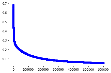
#训练第3个模型
w3,cost_lst3=grandient(data3_x,data3_y,iter_num,alpha)
plt.plot(range(iter_num),cost_lst3,"b-o")
[<matplotlib.lines.Line2D at 0x2562bcdfac0>]
#训练第4个模型
w4,cost_lst4=grandient(data4_x,data4_y,iter_num,alpha)
plt.plot(range(iter_num),cost_lst4,"b-o")
[<matplotlib.lines.Line2D at 0x25631ff4ee0>]
2.5 利用模型进行预测
data_x
array([[ 2.11663151e+00, 7.97280013e+00, -9.32896918e+00,-8.22460526e+00, -1.21784287e+01, 5.49844655e+00],[ 1.88644899e+00, 4.62100554e+00, 2.84159548e+00,4.31244563e-01, -2.47135027e+00, 2.50783257e+00],[ 2.39132949e+00, 6.46460915e+00, -9.80590050e+00,-7.28996786e+00, -9.65098460e+00, 6.38845956e+00],...,[ 2.03146167e+00, 7.80442707e+00, -8.53951210e+00,-9.82440872e+00, -1.00469351e+01, 6.91808489e+00],[ 4.08188906e+00, 6.12768483e+00, 1.10911262e+01,4.81201082e+00, -5.91530191e-03, 5.34221079e+00],[ 9.85744105e-01, 7.28573657e+00, -8.39593964e+00,-6.58647097e+00, -9.65176507e+00, 6.65101187e+00]])
data_x=np.insert(data_x,0,1,axis=1)
data_x.shape
(200, 7)
w3.shape
(7, 1)
multi_pred=pd.DataFrame(zip(h(data_x,w1).ravel(),h(data_x,w2).ravel(),h(data_x,w3).ravel(),h(data_x,w4).ravel()))
multi_pred
| 0 | 1 | 2 | 3 | |
|---|---|---|---|---|
| 0 | 0.020436 | 4.556248e-15 | 9.999975e-01 | 2.601227e-27 |
| 1 | 0.820488 | 4.180906e-05 | 3.551499e-05 | 5.908691e-05 |
| 2 | 0.109309 | 7.316201e-14 | 9.999978e-01 | 7.091713e-24 |
| 3 | 0.036608 | 9.999562e-01 | 1.048562e-09 | 5.724854e-03 |
| 4 | 0.003075 | 9.999292e-01 | 2.516742e-09 | 6.423038e-05 |
| ... | ... | ... | ... | ... |
| 195 | 0.017278 | 3.221293e-06 | 3.753372e-14 | 9.999943e-01 |
| 196 | 0.003369 | 9.999966e-01 | 6.673394e-10 | 2.281428e-03 |
| 197 | 0.000606 | 1.118174e-13 | 9.999941e-01 | 1.780212e-28 |
| 198 | 0.013072 | 4.999118e-05 | 9.811154e-14 | 9.996689e-01 |
| 199 | 0.151548 | 1.329623e-13 | 9.999447e-01 | 2.571989e-24 |
200 rows × 4 columns
2.6 计算准确率
np.sum(np.argmax(multi_pred.values,axis=1)==data_y.ravel())/len(data)
1.0
相关文章:
【Python机器学习】实验04(1) 多分类(基于逻辑回归)实践
文章目录 多分类以及机器学习实践如何对多个类别进行分类1.1 数据的预处理1.2 训练数据的准备1.3 定义假设函数,代价函数,梯度下降算法(从实验3复制过来)1.4 调用梯度下降算法来学习三个分类模型的参数1.5 利用模型进行预测1.6 评…...

【ChatGLM_01】ChatGLM2-6B本地安装与部署(大语言模型)
基于本地知识库的问答 1、简介(1)ChatGLM2-6B(2)LangChain(3)基于单一文档问答的实现原理(4)大规模语言模型系列技术:以GLM-130B为例(5)新建知识库…...
扫描器搭建扩展使用教程)
谷歌Tsunami(海啸)扫描器搭建扩展使用教程
目录 介绍 下载地址 功能总结 原理 服务探测 漏洞检测 安装...

诚迈科技承办大同首届信息技术产业峰会,共话数字经济崭新未来
7月28日,“聚势而强共领信创”2023大同首届信息技术产业峰会圆满举行。本次峰会由中共大同市委、大同市人民政府主办,中国高科技产业化研究会国际交流合作中心、山西省信创协会协办,中共大同市云冈区委、大同市云冈区人民政府、诚迈科技&…...
【Python】Python使用TK实现动态爱心效果
【Python】Python使用Tk实现动态爱心效果 画布使用了缓存机制,启动时绘制足够多的帧数,运行时一帧帧地取出来展示,明显更流畅,加快了程序执行速度。将控制跳动动画的函数从正弦函数换成了贝塞尔函数,贝塞尔函数更灵活…...

Unity3d C#快速打开萤石云监控视频流(ezopen)支持WebGL平台,替代UMP播放视频流的方案(含源码)
前言 Universal Media Player算是视频流播放功能常用的插件了,用到现在已经不知道躺了多少坑了,这个插件虽然是白嫖的,不过被甲方和领导吐槽的就是播放视频流的速度特别慢,可能需要几十秒来打开监控画面,等待的时间较…...
【Android】APP启动优化学习笔记
启动优化目的 用户体验: 应用的启动速度直接影响用户体验。用户希望应用能够快速启动并迅速响应他们的操作。如果应用启动较慢,用户可能会感到不满,并且有可能选择卸载或切换到竞争对手的应用。通过启动优化,可以提高应用的启动…...

docker的使用
docker安装 https://docs.docker.com/engine/install/debian/ 设置国内镜像 创建或修改 /etc/docker/daemon.json 文件,修改为如下形式 {"registry-mirrors": ["https://registry.hub.docker.com","http://hub-mirror.c.163.com"…...

iOS使用Rust调研
编辑已恢复 我们已与您断开连接。尝试重连时会保存您所做的变更。尝试重连 标题 1 已保存 Bin Song B 要发布此内容,请选择键盘上的 ⌘Enter。 发布 关闭 Rust技术空间 … 跨平台使用调研 iOS使用Rust调研 添加表情符号 添加标题图像 添加状态 一、iOS 项…...

抖音引流推广的几个方法,抖音全自动引流脚本软件详细使用教学
大家好我是你们的小编一辞脚本,今天给大家分享新的知识,很开心可以在CSDN平台分享知识给大家,很多伙伴看不到代码我先录制一下视频 在给大家做代码,给大家分享一下抖音引流脚本的知识和视频演示 不懂的小伙伴可以认真看一下,我们…...
k8s概念-DaemonSet
回到目录 参考链接https://v1-23.docs.kubernetes.io/zh/docs/concepts/workloads/controllers/daemonset/ DaemonSet 确保全部(或者某些)节点上运行一个 Pod 的副本 当节点加入到K8S集群中,pod会被(DaemonSet)调度到…...

Mac 终端快捷键设置:如何给 Mac 中的 Terminal 设置 Ctrl+Alt+T 快捷键快速启动
Mac 电脑中正常是没有直接打开终端命令行的快捷键指令的,但可以通过 commandspace 打开聚焦搜索,然后输入 ter 或者 terminal 全拼打开。但习惯了 linux 的同学会觉得这个操作很别扭。于是我们希望能通过键盘按键直接打开。 操作流程如下: 1…...
VR 变电站事故追忆反演——正泰电力携手图扑
VR(Virtual Reality,虚拟现实)技术作为近年来快速发展的一项新技术,具有广泛的应用前景,支持融合人工智能、机器学习、大数据等技术,实现更加智能化、个性化的应用。在电力能源领域,VR 技术在高性能计算机和专有设备支…...
fpga开发——蜂鸣器
蜂鸣器的原理 有源蜂鸣器和无源蜂鸣器 无源蜂鸣器利用电磁感应现象,为音圈接入交变电流后形成的电磁铁与永磁铁相吸或相斥而推动振膜发声,接入直流电只能持续推动振膜而无法产生声音,只能在接通或断开时产生声音。无源蜂鸣器的工作原理与扬声…...

【Liux下6818开发板(ARM)】触摸屏
(꒪ꇴ꒪ ),hello我是祐言博客主页:C语言基础,Linux基础,软件配置领域博主🌍快上🚘,一起学习!送给读者的一句鸡汤🤔:集中起来的意志可以击穿顽石!作者水平很有限,如果发现错误&#x…...

苍穹外卖day11——数据统计图形报表(Apache ECharts)
效果展示 Apache ECharts 介绍 常见图表 入门案例 快速上手 - Handbook - Apache ECharts 营业额统计——需求分析与设计 产品原型 接口设计 VO设计 营业额统计——代码开发 Controller中 /*** 数据统计相关接口*/ RestController RequestMapping("/admin/report&qu…...

在制作PC端Game Launcher游戏启动器时涉及到的技术选型
1)在制作PC端Game Launcher游戏启动器时涉及到的技术选型 2)如何将图片显示到Canvas的Raw Image上面 3)Unity 2018.4.4f1退出重启后出现黑屏 4)如何获取到GPU耗时 这是第346篇UWA技术知识分享的推送,精选了UWA社区…...
)
SQL力扣练习(九)
目录 1.订单最多的用户(586) 示例 1 解法一(limit) 解法二(dense_rank()) 2.体育馆的人流量 示例 1 解法一(临时表) 解法二(三表法) 1.订单最多的用户(586) 表: Orders --------------------------- | Column Name | Type | ---------…...

软考高级架构师笔记-10数学计算题
目录 1. 前文回顾 & 考情分析2. 最小生成树3. 最短路径4. 网络与最大流量5. 线性规划6. 动态规划/决策表7. 博弈论8. 状态转移矩阵9. 决策论10. 结语1. 前文回顾 & 考情分析 前文回顾: 软考高级架构师笔记-1计算机硬件软考高级架构师笔记-2计算机软件(操作系统)软考…...
)
设计模式五:建造者模式(Builder Pattern)
建造者模式(Builder Pattern)是一种创建型设计模式,用于通过一系列步骤来构建复杂对象。它将对象的构建过程与其表示分离,从而允许相同的构建过程可以创建不同的表示。 建造者模式中的几个角色: 产品(Product):表示被构建的复杂…...

连锁品牌万店扩张的破局之道:用数字化营建体系,突破规模化瓶颈
在消费市场竞争日趋激烈的当下,连锁品牌的规模化扩张,早已不是 “砸钱就能跑通” 的简单命题。很多品牌手握充足资金,却在扩张到几十、上百家门店时陷入停滞:门店营建标准混乱、多项目统筹失控、资深项目经理一将难求,…...
的开发详解五:SigmaStudio实战技巧与模块高效应用)
ADAU1701(含A2B)的开发详解五:SigmaStudio实战技巧与模块高效应用
1. SigmaStudio模块查找的终极技巧 第一次打开SigmaStudio时,面对左侧密密麻麻的模块列表,我完全懵了。就像走进一个巨大的图书馆却找不到分类标签,ADI把200多个算法模块分散在30多个分类里,光Volume Controls下面就有12种音量调节…...

使用VSCode无法登录Codex解决方法
登录时提示:Token exchange failed: token endpoint returned status 403 Forbidden: Country, region, or territory not supported确保魔法工具的连接模式是支持应用的,有的是只支持网站,切换成支持应用模式即可解决此问题。...
)
LabelImg标注的YOLO格式txt坐标转换保姆级教程(附Python代码)
LabelImg标注的YOLO格式坐标转换实战指南:从原理到Python实现 在计算机视觉项目中,数据标注是模型训练前的关键步骤。LabelImg作为一款开源的图像标注工具,支持生成YOLO格式的标注文件。然而,许多开发者在实际应用中发现ÿ…...
 2026)
Austroads:速度管理证据与指导回顾(英) 2026
这份报告是澳大利亚和新西兰道路运输委员会(Austroads)2025 年发布的《车速管理证据与指南回顾》,核心是为更新《道路安全指南:安全车速》(AGRS Part 3)梳理研究证据、 stakeholder 反馈并给出修订建议。下…...

DayZ社区离线模式:5步搭建专属单人末日世界
DayZ社区离线模式:5步搭建专属单人末日世界 【免费下载链接】DayZCommunityOfflineMode A community made offline mod for DayZ Standalone 项目地址: https://gitcode.com/gh_mirrors/da/DayZCommunityOfflineMode DayZ社区离线模式为玩家提供了一个完整的…...

如何解决神界原罪2模组冲突问题:Divinity Mod Manager终极指南
如何解决神界原罪2模组冲突问题:Divinity Mod Manager终极指南 【免费下载链接】DivinityModManager A mod manager for Divinity: Original Sin - Definitive Edition. 项目地址: https://gitcode.com/gh_mirrors/di/DivinityModManager Divinity Mod Manag…...

【ElevenLabs尼泊尔文语音实战指南】:20年AI语音工程师亲授7大避坑要点与本地化部署全流程
更多请点击: https://intelliparadigm.com 第一章:ElevenLabs尼泊尔文语音技术概览与核心价值 ElevenLabs 自 2023 年起逐步扩展其多语言语音合成能力,尼泊尔文(Nepali, ISO 639-1: ne)作为首批支持的南亚语系之一&am…...

技能同步工具:跨平台开发环境配置自动化管理方案
1. 项目概述:技能同步,一个被低估的开发者效率工具如果你和我一样,每天需要在多台电脑(比如公司的台式机、家里的笔记本、甚至偶尔应急的平板)之间切换,并且每台设备上都配置了不同的开发环境、安装了不同的…...

从“记录系统”到“智能系统” From “System of Record” to “System of Intelligence” —— A16Z
From “System of Record” to “System of Intelligence” 从“记录系统”到“智能系统” https://www.a16z.news/p/from-system-of-record-to-system-of Here’s one way you can think about system of record stickiness: For a long time, the valuable part of social…...