【小沐学NLP】关联规则分析Apriori算法(Mlxtend库,Python)
文章目录
- 1、简介
- 2、Mlxtend库
- 2.1 安装
- 2.2 功能
- 2.2.1 User Guide
- 2.2.2 User Guide - data
- 2.2.3 User Guide - frequent_patterns
- 2.3 入门示例
- 3、Apriori算法
- 3.1 基本概念
- 3.2 apriori
- 3.2.1 示例 1 -- 生成频繁项集
- 3.2.2 示例 2 -- 选择和筛选结果
- 3.2.3 示例 3 -- 使用稀疏表示
- 3.3 association_rules
- 3.3.1 示例 1 -- 从频繁项集生成关联规则
- 3.3.2 示例 2 -- 规则生成和选择标准
- 3.3.3 示例 3 -- 具有不完整的先前和后续信息的频繁项集
- 3.3.4 示例 4 -- 修剪关联规则
- 结语
1、简介
官网地址:
https://rasbt.github.io/mlxtend/
Mlxtend (machine learning extensions) is a Python library of useful tools for the day-to-day data science tasks.
关联规则分析是数据挖掘中最活跃的研究方法之一,目的是在一个数据集中找到各项之间的关联关系,而这种关系并没有在数据中直接体现出来。各种关联规则分析算法从不同方面入手减少可能的搜索空间大小以及减少扫描数据的次数。Apriori算法是最经典的挖掘频繁项集的算法,第一次实现在大数据集上的可行的关联规则提取,其核心思想是通过连接产生候选项及其支持度,然后通过剪枝生成频繁项集。
关联规则(Association Rules)是海量数据挖掘(Mining Massive Datasets,MMDs)非常经典的任务,其主要目标是试图从一系列事务集中挖掘出频繁项以及对应的关联规则。关联规则来自于一个家喻户晓的“啤酒与尿布”的故事。

2、Mlxtend库
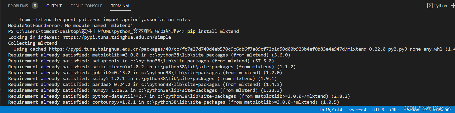
2.1 安装
pip install mlxtend
# or
pip install mlxtend --upgrade --no-deps
# or
pip install -i https://pypi.tuna.tsinghua.edu.cn/simple mlxtend
2.2 功能
2.2.1 User Guide
- classifier
- cluster
- data
- evaluate
- feature_extraction
- feature_selection
- file_io
- frequent_patterns
- image
- math
- plotting
- preprocessing
- regressor
- text
- utils
2.2.2 User Guide - data
- autompg_data
The Auto-MPG dataset for regression.
A function that loads the autompg dataset into NumPy arrays.
from mlxtend.data import autompg_data
X, y = autompg_data()print('Dimensions: %s x %s' % (X.shape[0], X.shape[1]))
print('\nHeader: %s' % ['cylinders', 'displacement', 'horsepower', 'weight', 'acceleration','model year', 'origin', 'car name'])
print('1st row', X[0])
- boston_housing_data
The Boston housing dataset for regression.
A function that loads the boston_housing_data dataset into NumPy arrays.
from mlxtend.data import boston_housing_data
X, y = boston_housing_data()print('Dimensions: %s x %s' % (X.shape[0], X.shape[1]))
print('1st row', X[0])
- iris_data
The 3-class iris dataset for classification
A function that loads the iris dataset into NumPy arrays.
from mlxtend.data import iris_data
X, y = iris_data()print('Dimensions: %s x %s' % (X.shape[0], X.shape[1]))
print('\nHeader: %s' % ['sepal length', 'sepal width','petal length', 'petal width'])
print('1st row', X[0])
import numpy as np
print('Classes: Setosa, Versicolor, Virginica')
print(np.unique(y))
print('Class distribution: %s' % np.bincount(y))
- loadlocal_mnist
A function for loading MNIST from the original ubyte files
A utility function that loads the MNIST dataset from byte-form into NumPy arrays.
from mlxtend.data import loadlocal_mnist
import platform
if not platform.system() == 'Windows':X, y = loadlocal_mnist(images_path='train-images-idx3-ubyte', labels_path='train-labels-idx1-ubyte')else:X, y = loadlocal_mnist(images_path='train-images.idx3-ubyte', labels_path='train-labels.idx1-ubyte')
print('Dimensions: %s x %s' % (X.shape[0], X.shape[1]))
print('\n1st row', X[0])
import numpy as npprint('Digits:  0 1 2 3 4 5 6 7 8 9')
print('labels: %s' % np.unique(y))
print('Class distribution: %s' % np.bincount(y))
- make_multiplexer_dataset
A function for creating multiplexer data
Function that creates a dataset generated by a n-bit Boolean multiplexer for evaluating supervised learning algorithms.
import numpy as np
from mlxtend.data import make_multiplexer_datasetX, y = make_multiplexer_dataset(address_bits=2, sample_size=10,positive_class_ratio=0.5, shuffle=False,random_seed=123)print('Features:\n', X)
print('\nClass labels:\n', y)
- mnist_data
A subset of the MNIST dataset for classification
A function that loads the MNIST dataset into NumPy arrays.
from mlxtend.data import mnist_data
X, y = mnist_data()print('Dimensions: %s x %s' % (X.shape[0], X.shape[1]))
print('1st row', X[0])
- three_blobs_data
The synthetic blobs for classification
A function that loads the three_blobs dataset into NumPy arrays.
from mlxtend.data import three_blobs_data
X, y = three_blobs_data()print('Dimensions: %s x %s' % (X.shape[0], X.shape[1]))
print('1st row', X[0])
import numpy as npprint('Suggested cluster labels')
print(np.unique(y))
print('Label distribution: %s' % np.bincount(y))
import matplotlib.pyplot as pltplt.scatter(X[:,0], X[:,1],c='white',marker='o',s=50)plt.grid()
plt.show()
- wine_data
A 3-class wine dataset for classification
A function that loads the Wine dataset into NumPy arrays.
from mlxtend.data import wine_data
X, y = wine_data()print('Dimensions: %s x %s' % (X.shape[0], X.shape[1]))
print('\nHeader: %s' % ['alcohol', 'malic acid', 'ash', 'ash alcalinity','magnesium', 'total phenols', 'flavanoids','nonflavanoid phenols', 'proanthocyanins','color intensity', 'hue', 'OD280/OD315 of diluted wines','proline'])
print('1st row', X[0])
import numpy as np
print('Classes: %s' % np.unique(y))
print('Class distribution: %s' % np.bincount(y))
2.2.3 User Guide - frequent_patterns
- apriori
(1)通过Apriori算法的频繁项集,用于提取频繁项集以进行关联规则挖掘的先验函数。
(2)Apriori 是一种流行的算法,用于提取具有关联规则学习应用的频繁项集。先验算法被设计为在包含交易的数据库上运行,例如商店顾客的购买。如果项集满足用户指定的支持阈值(support threshold),则将其视为“频繁”。例如,如果支持阈值(support threshold)设置为 0.5 (50%),则常用项集定义为在数据库中至少 50% 的事务中一起出现的一组项。
from mlxtend.frequent_patterns import aprioriapriori(df, min_support=0.5, use_colnames=False, max_len=None, verbose=0, low_memory=False)
- association_rules
从频繁项集生成关联规则,从频繁项集生成关联规则的函数。
from mlxtend.frequent_patterns import association_rules# 生成关联规则的数据帧,包括 指标“得分”、“置信度”和“提升”
association_rules(df, metric='confidence', min_threshold=0.8, support_only=False)
- fpgrowth
(1)通过 FP-growth 算法的频繁项集,实现 FP-Growth 以提取频繁项集以进行关联规则挖掘的函数。
(2)FP-Growth 是一种用于提取频繁项集的算法,其应用在关联规则学习中,成为已建立的先验算法的流行替代方案。- 通常,该算法被设计为在包含交易的数据库上运行,例如商店客户的购买。如果项集满足用户指定的支持阈值,则将其视为“频繁”。例如,如果支持阈值设置为 0.5 (50%),则常用项集定义为在数据库中至少 50% 的事务中一起出现的一组项。
- 特别是,与Apriori频繁模式挖掘算法的不同之处在于,FP-Growth是一种不需要生成候选模式的频繁模式挖掘算法。在内部,它使用所谓的FP树(频繁模式树)数据,而无需显式生成候选集,这对于大型数据集特别有吸引力。
from mlxtend.frequent_patterns import apriori# Get frequent itemsets from a one-hot DataFrame
fpgrowth(df, min_support=0.5, use_colnames=False, max_len=None, verbose=0)
- fpmax
(1)通过 FP-Max 算法实现的最大项集,实现 FP-Max 以提取最大项集以进行关联规则挖掘的函数。
(2)Apriori 算法是用于频繁生成项集的最早也是最流行的算法之一(然后频繁项集用于关联规则挖掘)。但是,Apriori 的运行时可能非常大,特别是对于具有大量唯一项的数据集,因为运行时会根据唯一项的数量呈指数级增长。- 与Apriori相比,FP-Growth 是一种频繁的模式生成算法,它将项目插入到模式搜索树中,这允许它在运行时相对于唯一项目或条目的数量线性增加。
- FP-Max是FP-Growth的变体,专注于获取最大项集。如果 X 频繁且不存在包含 X 的频繁超模式,则称项集 X 为最大值。换句话说,频繁模式 X 不能是较大频繁模式的子模式,以符合定义最大项集。
from mlxtend.frequent_patterns import apriori# Get maximal frequent itemsets from a one-hot DataFrame
fpmax(df, min_support=0.5, use_colnames=False, max_len=None, verbose=0)
2.3 入门示例
import numpy as np
import matplotlib.pyplot as plt
import matplotlib.gridspec as gridspec
import itertools
from sklearn.linear_model import LogisticRegression
from sklearn.svm import SVC
from sklearn.ensemble import RandomForestClassifier
from mlxtend.classifier import EnsembleVoteClassifier
from mlxtend.data import iris_data
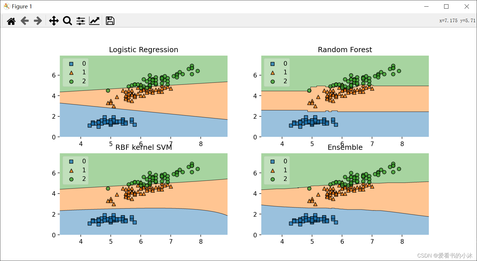
from mlxtend.plotting import plot_decision_regions# Initializing Classifiers
clf1 = LogisticRegression(random_state=0)
clf2 = RandomForestClassifier(random_state=0)
clf3 = SVC(random_state=0, probability=True)
eclf = EnsembleVoteClassifier(clfs=[clf1, clf2, clf3],weights=[2, 1, 1], voting='soft')# Loading some example data
X, y = iris_data()
X = X[:,[0, 2]]# Plotting Decision Regionsgs = gridspec.GridSpec(2, 2)
fig = plt.figure(figsize=(10, 8))labels = ['Logistic Regression','Random Forest','RBF kernel SVM','Ensemble']for clf, lab, grd in zip([clf1, clf2, clf3, eclf],labels,itertools.product([0, 1],repeat=2)):clf.fit(X, y)ax = plt.subplot(gs[grd[0], grd[1]])fig = plot_decision_regions(X=X, y=y,clf=clf, legend=2)plt.title(lab)plt.show()
3、Apriori算法
3.1 基本概念
-
关联规则的一般形式
- 关联规则的支持度(相对支持度)
项集A、B同时发生的概率称为关联规则的支持度(相对支持度)。Support(A=>B)=P(A∪B) - 关联规则的置信度
项集A发生,则项集B发生的概率为关联规则的置信度。Confidence(A=>B)=P(B∣A)
- 关联规则的支持度(相对支持度)
-
最小支持度和最小置信度
- 最小支持度是衡量支持度的一个阈值,表示项目集在统计意义上的最低重要性
- 最小置信度是衡量置信度的一个阈值,表示关联规则的最低可靠性
- 强规则是同时满足最小支持度阈值和最小置信度阈值的规则
-
项集
- 项集是项的集合。包含k 个项的集合称为k 项集
- 项集出现的频率是所有包含项集的事务计数,又称为绝对支持度或支持度计数
- 如果项集的相对支持度满足预定义的最小支持度阈值,则它是频繁项集。
-
支持度计数
- 项集A的支持度计数是事务数据集中包含项集A的事务个数,简称项集的频率或计数
- 一旦得到项集A 、 B 和A∪B的支持度计数以及所有事务个数,就可以导出对应的关联规则A=>B和B=>A,并可以检查该规则是否为强规则。
关联分析(Association Analysis):在大规模数据集中寻找有趣的关系。
频繁项集(Frequent Item Sets):经常出现在一块的物品的集合,即包含0个或者多个项的集合称为项集。
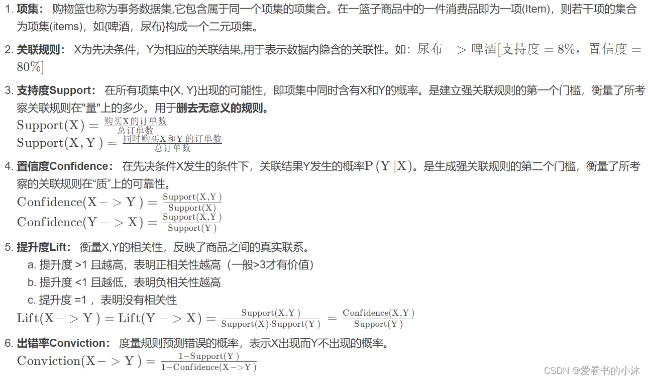
支持度(Support):数据集中包含该项集的记录所占的比例,是针对项集来说的。
置信度(Confidence):出现某些物品时,另外一些物品必定出现的概率,针对规则而言。
关联规则(Association Rules):暗示两个物品之间可能存在很强的关系。形如A->B的表达式,规则A->B的度量包括支持度和置信度
项集支持度:一个项集出现的次数与数据集所有事物数的百分比称为项集的支持度支持度: 首先是个百分比值,指的是某个商品组合出现的次数与总次数之间的比例。支持度越高,代表这个组合(可以是单个商品)出现的频率越大。
置信度:首先是个条件概率。指的是当你购买了商品A,会有多大的概率购买商品B
提升度: 商品A的出现,对商品B的出现概率提升的程度。提升度(A→B)=置信度(A→B)/支持度(B)什么样的数据才是频繁项集呢?从名字上来看就是出现次数多的集合,没错,但是上面算次数多呢?这里我们给出频繁项集的定义。**频繁项集:**支持度大于等于最小支持度(Min Support)阈值的项集。
1、导入数据,并将数据预处理
2、计算频繁项集
3、根据各个频繁项集,分别计算支持度和置信度
4、根据提供的最小支持度和最小置信度,输出满足要求的关联规则
(1)找出频繁项集(支持度必须大于等于给定的最小支持度阈值)
生成频繁项目集。
一个频繁项集的所有子集必须也是频繁的。
指定最小支持度(min_support),过滤掉非频繁项集,既能减轻计算负荷又能提高预测质量。
(2)找出上步中频繁项集的规则
生成关联规则。
指定最小置信度(metric = “confidence”, min_threshold = 0.01),来过滤掉弱规则。
由频繁项集产生强关联规则。由第一步可知,未超过预定的最小支持阈值的项集已被剔除,如果剩下的这些项集又满足了预定的最小置信度阈值,那么就挖掘出了强关联规则。
(3)Metrics
- ‘support’:

- ‘confidence’:

- ‘lift’:

- ‘leverage’:

- ‘conviction’:

- ‘zhangs_metric’:

Apriori算法的主要思想是找出存在于事务数据集中最大的频繁项集,再利用得到的最大频繁项集与预先设定的最小置信度阈值生成强关联规则。频繁项集的所有非空子集一定是频繁项集。
Apriori算法流程:
1、首先对数据库中进行一次扫描,统计每一个项出现的次数,形成候选1-项集;
2、根据minsupport阈值筛选出频繁1-项集;
3、将频繁1-项集进行组合,形成候选2-项集;
4、对数据库进行第二次扫描,为每个候选2-项集进行计数,并筛选出频繁2-项集;
5、重复上述流程,直到候选项集为空;
6、根据生成的频繁项集,通过计算相应的置信度来生成管理规则。
3.2 apriori
Frequent itemsets via the Apriori algorithm.
Apriori function to extract frequent itemsets for association rule mining.
3.2.1 示例 1 – 生成频繁项集
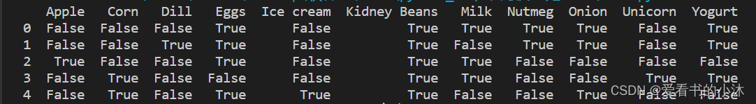
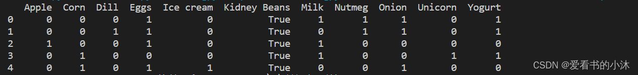
- 我们可以通过以下方式将其转换为正确的格式:TransactionEncoder
dataset = [['Milk', 'Onion', 'Nutmeg', 'Kidney Beans', 'Eggs', 'Yogurt'],['Dill', 'Onion', 'Nutmeg', 'Kidney Beans', 'Eggs', 'Yogurt'],['Milk', 'Apple', 'Kidney Beans', 'Eggs'],['Milk', 'Unicorn', 'Corn', 'Kidney Beans', 'Yogurt'],['Corn', 'Onion', 'Onion', 'Kidney Beans', 'Ice cream', 'Eggs']]import pandas as pd
from mlxtend.preprocessing import TransactionEncoderte = TransactionEncoder()
te_ary = te.fit(dataset).transform(dataset)
df = pd.DataFrame(te_ary, columns=te.columns_)
print(df)
- 现在,让我们返回至少具有 60% 支持的项和项集:
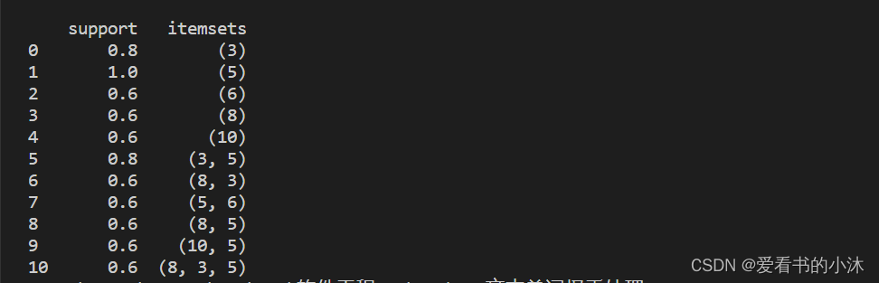
from mlxtend.frequent_patterns import apriorifrequent_itemsets = apriori(df, min_support=0.6)
print(frequent_itemsets)
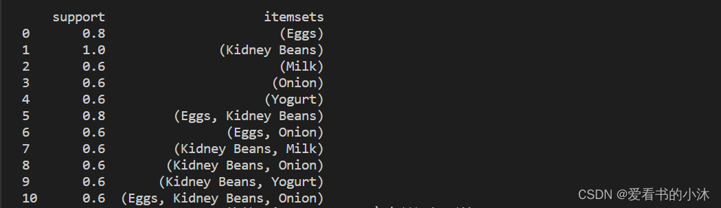
- 默认情况下, 返回项的列索引,这在下游操作(如关联规则挖掘)中可能很有用。为了更好的可读性,我们可以设置将这些整数值转换为相应的项目名称:aprioriuse_colnames=True
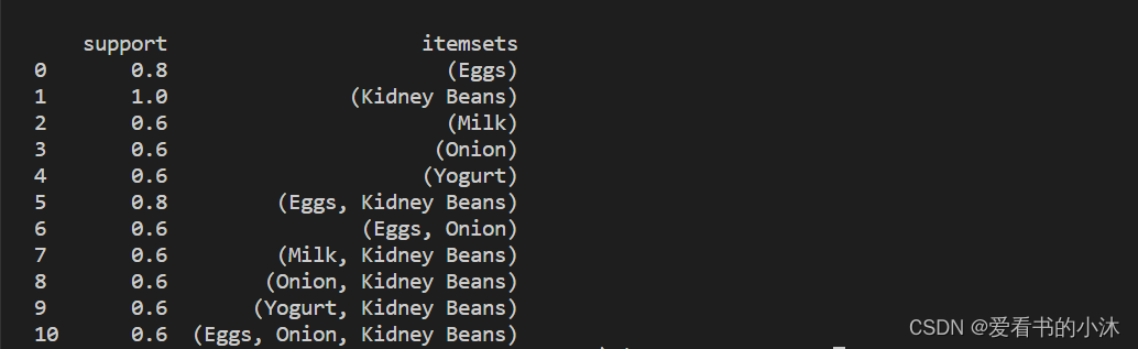
from mlxtend.frequent_patterns import apriorifrequent_itemsets = apriori(df, min_support=0.6, use_colnames=True)
print(frequent_itemsets)
3.2.2 示例 2 – 选择和筛选结果
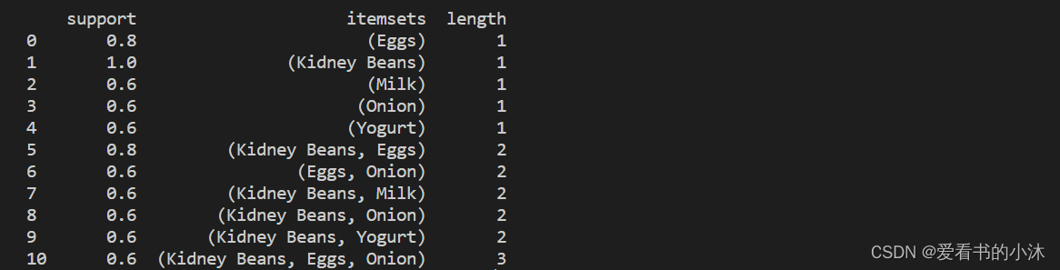
- 在于我们可以使用pandas它方便的功能来过滤结果。例如,假设我们只对长度为 2 且支持至少为 80% 的项集感兴趣。首先,我们通过创建频繁的项集,并添加一个新列来存储每个项集的长度.
from mlxtend.frequent_patterns import apriorifrequent_itemsets = apriori(df, min_support=0.6, use_colnames=True)
frequent_itemsets['length'] = frequent_itemsets['itemsets'].apply(lambda x: len(x))
print(frequent_itemsets)
- 然后,我们可以选择满足我们所需标准的结果,如下所示:
from mlxtend.frequent_patterns import apriorifrequent_itemsets = apriori(df, min_support=0.6, use_colnames=True)
frequent_itemsets['length'] = frequent_itemsets['itemsets'].apply(lambda x: len(x))
frequent_itemsets = frequent_itemsets[ (frequent_itemsets['length'] == 2) & (frequent_itemsets['support'] >= 0.8) ]
print(frequent_itemsets)

- 同样,使用 Pandas API,我们可以根据“项集”列选择条目:
from mlxtend.frequent_patterns import apriorifrequent_itemsets = apriori(df, min_support=0.6, use_colnames=True)
frequent_itemsets['length'] = frequent_itemsets['itemsets'].apply(lambda x: len(x))
frequent_itemsets = frequent_itemsets[ frequent_itemsets['itemsets'] == {'Onion', 'Eggs'} ]
print(frequent_itemsets)

3.2.3 示例 3 – 使用稀疏表示
- 为了节省内存,您可能希望以稀疏格式表示事务数据。
import pandas as pd
from mlxtend.preprocessing import TransactionEncoderte = TransactionEncoder()
oht_ary = te.fit(dataset).transform(dataset, sparse=True)
sparse_df = pd.DataFrame.sparse.from_spmatrix(oht_ary, columns=te.columns_)
print(sparse_df)
import pandas as pd
from mlxtend.preprocessing import TransactionEncoder
from mlxtend.frequent_patterns import apriorite = TransactionEncoder()
oht_ary = te.fit(dataset).transform(dataset, sparse=True)
sparse_df = pd.DataFrame.sparse.from_spmatrix(oht_ary, columns=te.columns_)
# print(sparse_df)frequent_itemsets = apriori(sparse_df, min_support=0.6, use_colnames=True, verbose=1)
print(frequent_itemsets)
3.3 association_rules
Association rules generation from frequent itemsets.
Function to generate association rules from frequent itemsets.
3.3.1 示例 1 – 从频繁项集生成关联规则
- 我们首先创建一个由 fpgrowth 函数生成的频繁项集的pandas.
import pandas as pd
from mlxtend.preprocessing import TransactionEncoder
from mlxtend.frequent_patterns import apriori, fpmax, fpgrowthdataset = [['Milk', 'Onion', 'Nutmeg', 'Kidney Beans', 'Eggs', 'Yogurt'],['Dill', 'Onion', 'Nutmeg', 'Kidney Beans', 'Eggs', 'Yogurt'],['Milk', 'Apple', 'Kidney Beans', 'Eggs'],['Milk', 'Unicorn', 'Corn', 'Kidney Beans', 'Yogurt'],['Corn', 'Onion', 'Onion', 'Kidney Beans', 'Ice cream', 'Eggs']]te = TransactionEncoder()
te_ary = te.fit(dataset).transform(dataset)
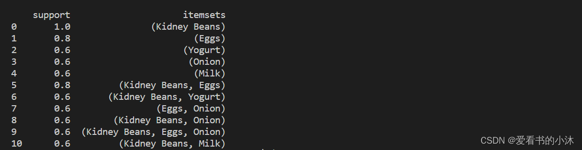
df = pd.DataFrame(te_ary, columns=te.columns_)frequent_itemsets = fpgrowth(df, min_support=0.6, use_colnames=True)
### alternatively:
#frequent_itemsets = apriori(df, min_support=0.6, use_colnames=True)
#frequent_itemsets = fpmax(df, min_support=0.6, use_colnames=True)print(frequent_itemsets)
- 该函数允许您 (1) 指定您感兴趣的指标和 (2) 相应的阈值。目前实施的措施是信心和提升。假设,仅当置信度高于 70% 阈值 时,您才对从频繁项集派生的规则感兴趣。
from mlxtend.frequent_patterns import association_rulesrules = association_rules(frequent_itemsets, metric="confidence", min_threshold=0.7)
print(rules)
3.3.2 示例 2 – 规则生成和选择标准
如果您对根据不同兴趣指标的规则感兴趣,您可以简单地调整和参数。例如,如果您只对提升分数为 >= 1.2 的规则感兴趣,则可以执行以下操作:
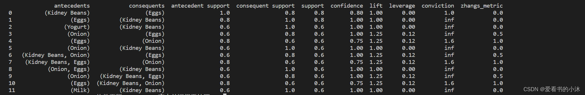
from mlxtend.frequent_patterns import association_rulesrules = association_rules(frequent_itemsets, metric="lift", min_threshold=1.2)
print(rules)

我们可以按如下方式计算先行长度:
from mlxtend.frequent_patterns import association_rulesrules = association_rules(frequent_itemsets, metric="lift", min_threshold=1.2)
# print(rules)
rules["antecedent_len"] = rules["antecedents"].apply(lambda x: len(x))
print(rules)

假设我们对满足以下条件的规则感兴趣:
- 至少 2 个前因
- 置信度> 0.75
- 提升得分> 1.2
from mlxtend.frequent_patterns import association_rulesrules = association_rules(frequent_itemsets, metric="lift", min_threshold=1.2)
# print(rules)
rules["antecedent_len"] = rules["antecedents"].apply(lambda x: len(x))
# print(rules)
rules = rules[ (rules['antecedent_len'] >= 2) &(rules['confidence'] > 0.75) &(rules['lift'] > 1.2) ]
print(rules)

同样,使用 Pandas API,我们可以根据“前因”或“后因”列选择条目:
from mlxtend.frequent_patterns import association_rulesrules = association_rules(frequent_itemsets, metric="lift", min_threshold=1.2)
# print(rules)
rules["antecedent_len"] = rules["antecedents"].apply(lambda x: len(x))
# print(rules)
rules[rules['antecedents'] == {'Eggs', 'Kidney Beans'}]
print(rules)

3.3.3 示例 3 – 具有不完整的先前和后续信息的频繁项集
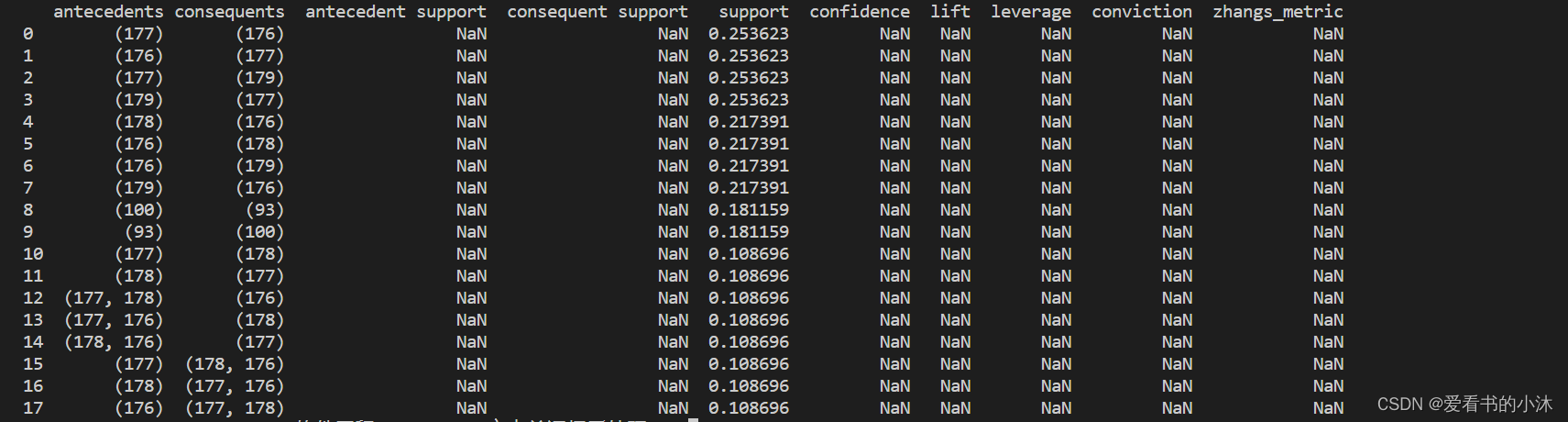
计算的大多数指标取决于频繁项集输入数据帧中提供的给定规则的结果和先前支持分数。
import pandas as pddict = {'itemsets': [['177', '176'], ['177', '179'],['176', '178'], ['176', '179'],['93', '100'], ['177', '178'],['177', '176', '178']],'support':[0.253623, 0.253623, 0.217391,0.217391, 0.181159, 0.108696, 0.108696]}freq_itemsets = pd.DataFrame(dict)
print(freq_itemsets)
import pandas as pddict = {'itemsets': [['177', '176'], ['177', '179'],['176', '178'], ['176', '179'],['93', '100'], ['177', '178'],['177', '176', '178']],'support':[0.253623, 0.253623, 0.217391,0.217391, 0.181159, 0.108696, 0.108696]}freq_itemsets = pd.DataFrame(dict)
print(freq_itemsets)from mlxtend.frequent_patterns import association_rules
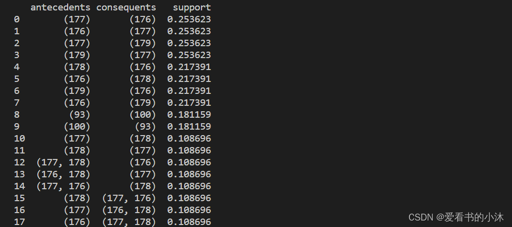
res = association_rules(freq_itemsets, support_only=True, min_threshold=0.1)
print(res)
import pandas as pddict = {'itemsets': [['177', '176'], ['177', '179'],['176', '178'], ['176', '179'],['93', '100'], ['177', '178'],['177', '176', '178']],'support':[0.253623, 0.253623, 0.217391,0.217391, 0.181159, 0.108696, 0.108696]}freq_itemsets = pd.DataFrame(dict)
print(freq_itemsets)from mlxtend.frequent_patterns import association_rules
res = association_rules(freq_itemsets, support_only=True, min_threshold=0.1)
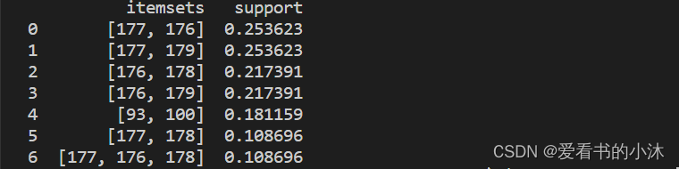
print(res)res = res[['antecedents', 'consequents', 'support']]
print(res)
3.3.4 示例 4 – 修剪关联规则
没有用于修剪的特定 API。相反,可以在生成的数据帧上使用 pandas API 来删除单个行。
import pandas as pd
from mlxtend.preprocessing import TransactionEncoder
from mlxtend.frequent_patterns import apriori, fpmax, fpgrowth
from mlxtend.frequent_patterns import association_rulesdataset = [['Milk', 'Onion', 'Nutmeg', 'Kidney Beans', 'Eggs', 'Yogurt'],['Dill', 'Onion', 'Nutmeg', 'Kidney Beans', 'Eggs', 'Yogurt'],['Milk', 'Apple', 'Kidney Beans', 'Eggs'],['Milk', 'Unicorn', 'Corn', 'Kidney Beans', 'Yogurt'],['Corn', 'Onion', 'Onion', 'Kidney Beans', 'Ice cream', 'Eggs']]te = TransactionEncoder()
te_ary = te.fit(dataset).transform(dataset)
df = pd.DataFrame(te_ary, columns=te.columns_)frequent_itemsets = fpgrowth(df, min_support=0.6, use_colnames=True)
rules = association_rules(frequent_itemsets, metric="lift", min_threshold=1.2)
print(rules)

我们想删除规则“(洋葱、芸豆)->(鸡蛋)”。为此,我们可以定义选择掩码并删除此行
import pandas as pd
from mlxtend.preprocessing import TransactionEncoder
from mlxtend.frequent_patterns import apriori, fpmax, fpgrowth
from mlxtend.frequent_patterns import association_rulesdataset = [['Milk', 'Onion', 'Nutmeg', 'Kidney Beans', 'Eggs', 'Yogurt'],['Dill', 'Onion', 'Nutmeg', 'Kidney Beans', 'Eggs', 'Yogurt'],['Milk', 'Apple', 'Kidney Beans', 'Eggs'],['Milk', 'Unicorn', 'Corn', 'Kidney Beans', 'Yogurt'],['Corn', 'Onion', 'Onion', 'Kidney Beans', 'Ice cream', 'Eggs']]te = TransactionEncoder()
te_ary = te.fit(dataset).transform(dataset)
df = pd.DataFrame(te_ary, columns=te.columns_)frequent_itemsets = fpgrowth(df, min_support=0.6, use_colnames=True)
rules = association_rules(frequent_itemsets, metric="lift", min_threshold=1.2)
print(rules)antecedent_sele = rules['antecedents'] == frozenset({'Onion', 'Kidney Beans'}) # or  frozenset({'Kidney Beans', 'Onion'})
consequent_sele = rules['consequents'] == frozenset({'Eggs'})
final_sele = (antecedent_sele & consequent_sele)rules = rules.loc[ ~final_sele ]
print(rules)
结语
如果您觉得该方法或代码有一点点用处,可以给作者点个赞,或打赏杯咖啡;╮( ̄▽ ̄)╭
如果您感觉方法或代码不咋地//(ㄒoㄒ)//,就在评论处留言,作者继续改进;o_O???
如果您需要相关功能的代码定制化开发,可以留言私信作者;(✿◡‿◡)
感谢各位大佬童鞋们的支持!( ´ ▽´ )ノ ( ´ ▽´)っ!!!
相关文章:
【小沐学NLP】关联规则分析Apriori算法(Mlxtend库,Python)
文章目录 1、简介2、Mlxtend库2.1 安装2.2 功能2.2.1 User Guide2.2.2 User Guide - data2.2.3 User Guide - frequent_patterns 2.3 入门示例 3、Apriori算法3.1 基本概念3.2 apriori3.2.1 示例 1 -- 生成频繁项集3.2.2 示例 2 -- 选择和筛选结果3.2.3 示例 3 -- 使用稀疏表示…...

对话ChatGPT:AIGC时代下,分布式存储的应用与前景
随着科技的飞速发展,我们正步入一个被称为AIGC时代的全新阶段,人工智能、物联网、大数据、云计算成为这个信息爆炸时代的主要特征。自2022年11月以来,ChatGPT的知名度迅速攀升,引发了全球科技爱好者的极大关注,其高超的…...

java多线程学习笔记一
一、线程的概述 1.1 线程的相关概念 1.1.1 进程(Process) 进程(Process)是计算机的程序关于某数据集合上的一次运行活动,是操作系统进行资源分配与调度的基本单位。 可以把进程简单的理解为操作系统中正在有运行的一…...
BOM与DOM--记录
BOM基础(BOM简介、常见事件、定时器、this指向) BOM和DOM的区别和联系 JavaScript的DOM与BOM的区别与用法详解 DOM和BOM是什么?有什么作用? 图解BOM与DOM的区别与联系 BOM和DOM详解 JavaScript 中的 BOM(浏览器对…...
Docker安装MongoDB
一、docker安装mongodb MongoDB 是一个免费的开源跨平台面向文档的 NoSQL 数据库程序。 二、安装步骤 1.docker 拉取mysql镜像 docker pull mongo:latest 2.运行容器 docker run -itd --name mongo -p 27017:27017 mongo --auth参数说明: -p 27017:27017 &#…...

不要对正则表达式进行频繁重复预编译
背景 在频繁调用场景,如方法体内或者循环语句中,新定义Pattern会导致重复预编译正则表达式,降低程序执行效率。另外,在 JDK 中部分 入参为正则表达式格式的 API,如 String.replaceAll, String.split 等,也…...

vue入门及小项目小便签条
vue 框架:是一个半成品软件,是一套可重用的,通用的,软件基础代码模型。基于框架进行开发,更加快捷 ,更加高效 v-bind为HTML标签绑定属性值,如设置href,css样式等 v-model在表单元素上创建双向数…...
详解TCP/IP协议第四篇:数据在网络中传输方式的分类概述
文章目录 前言 一:面向有连接型与面向无连接型 1:大致概念 2:面向有连接型 3:面向无连接型 二:电路交换与分组交换 1:分组交换概念 2:分组交交换过程 三:根据接收端数量分…...

SpringMvc决战-【SpringMVC之自定义注解】
目录 一、前言 1.1.什么是注解 1.2.注解的用处 1.3.注解的原理 二.注解父类 1.注解包括那些 2.JDK基本注解 3. JDK元注解 4.自定义注解 5.如何使用自定义注解(包括:注解标记【没有任何东西】,元数据注解)? 三…...
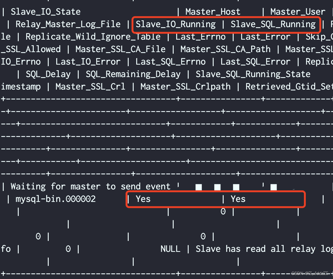
【MySQL集群一】CentOS 7上搭建MySQL集群:一主一从、多主多从
CentOS 7上搭建MySQL集群 介绍一主一从步骤1:准备工作步骤2:安装MySQL步骤3:配置主服务器步骤4:创建复制用户步骤5:备份主服务器数据,如果没有数据则省略这一步步骤6:配置从服务器步骤7…...
RGB格式
Qt视频播放器实现(目录) RGB的使用场景 目前,数字信号源(直播现场的数字相机采集的原始画面)和显示设备(手机屏幕、笔记本屏幕、个人电脑显示器屏幕)使用的基本上都是RGB格式。 三原色 RGB是…...
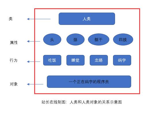
认识面向对象-PHP8知识详解
面向对象编程,也叫面向对象程序设计,是在面向过程程序设计的基础上发展而来的,它比面向过程编程具有更强的灵活性和扩展性。 它用类、对象、关系、属性等一系列东西来提高编程的效率,其主要的特性是可封装性、可继承性和多态性。…...
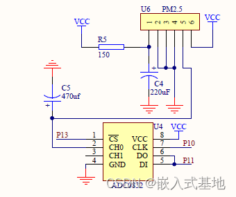
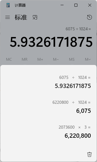
毕业设计|基于51单片机的空气质量检测PM2.5粉尘检测温度设计
基于51单片机的空气质量检测PM2.5粉尘检测温度设计 1、项目简介1.1 系统构成1.2 系统功能 2、部分电路设计2.1 LED信号指示灯电路设计2.2 LCD1602显示电路2.3 PM2.5粉尘检测电路设计 3、部分代码展示3.1 串口初始化3.1 定时器初始化3.2 LCD1602显示函数 4 演示视频及代码资料获…...

星闪空口技术初探
星闪技术设计目标 在星闪技术的应用场景中,最低的时延要求达到了20us量级,比如智能座舱的主动降噪。最高的可靠性要求达到了99.9999%,比如智能制造的传感器与执行器的消息收发。除了低时延和高可靠之外,高精度同步、多并发和信息…...

如何在不失去理智的情况下调试 TensorFlow 训练程序
一、说明 关于tensorflow的调试,是一个难啃的骨头,除了要有耐力,还需要方法;本文假设您是一个很有耐力的开发者,为您提供一些方法;这些方法也许不容易驾驭,但是依然强调您只要有耐力,…...
24. 图论 - 图的表示种类
Hi,你好。我是茶桁。 之前的一节课中,我们了解了图的来由和构成,简单的理解了一下图的一些相关概念。那么这节课,我们要了解一下图的表示,种类。相应的,我们中间需要穿插一些新的知识点用于更好的去理解图…...

C++ 读bin文件,部分代码。赚经验。
编号:1 Head: magicWord[0] 0x0102 magicWord[1] 0x0304 magicWord[2] 0x0506 magicWord[3] 0x0708 version 0x02010004 totalPacketLen 288 platform 0x000a1443 frameNumber 12 timeCpuCycles 172969774 numDetectedObj 99 numTLVs 2 subFrameNumber 0 TLV…...

vue3 父子组件传值
一,子传父 父组件 <script setup> import HelloWorld from ./components/HelloWorld.vue import { ref } from vue//直接赋值页面不会自动渲染,使用ref存储响应式数据 import { defineExpose } from "vue";父传子 let val ref(); con…...
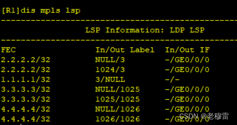
【看懂MPLS LSP表项】
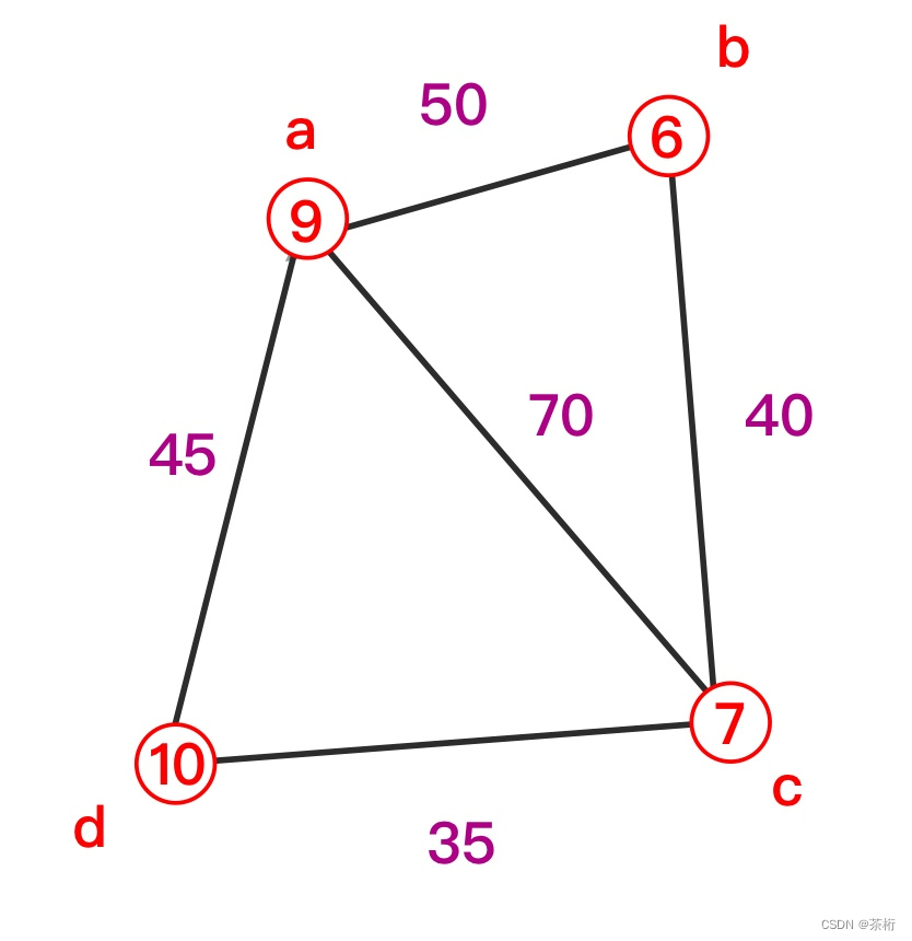
IP网络 R1根据路由表项去查FIB表 目的网络、出口、下一跳 MPLS网络 R1根据LFIB表现去查表, 路由,出口、(标签) 要实现MPLS网络全局可达性,R1应具有到每一个LSR、LSE的路由。 1、R1去FEC(转发等价类) /去往2.2.2.2的路由《路由方…...

代码随想录训练营 单调栈
代码随想录训练营 单调栈 84. 柱状图中最大的矩形🌸 最后一天~ 84. 柱状图中最大的矩形🌸 给定 n 个非负整数,用来表示柱状图中各个柱子的高度。每个柱子彼此相邻,且宽度为 1 。 求在该柱状图中,能够勾勒出来的矩形的最…...

深入解析 Android 开发高级工程师:职责、技能与面试精要
在移动互联网时代,Android 平台作为全球最大的移动操作系统之一,其应用开发人才的需求持续旺盛。对于追求技术深度和业务影响力的开发者而言,进阶成为 Android 开发高级工程师是一个重要的里程碑。这不仅要求开发者具备扎实的编码功底和丰富的项目经验,更需要其在架构设计、…...

Janus-Pro-7B WebUI开发进阶:利用JavaScript打造动态交互界面
Janus-Pro-7B WebUI开发进阶:利用JavaScript打造动态交互界面 1. 引言:从静态展示到动态交互 如果你用过一些大模型的基础Web界面,可能会觉得它们有点“呆”。输入问题,等待,然后一次性看到所有答案。整个过程就像在…...

PrivLLM 协变混淆:隐私保护的 LLM 推理高效实现
用户接入云上大模型(LLM)时,通常面临端-云数据交互如提示词上传等隐私泄露风险。常规脱敏和加密手段难以同时保障数据安全隐私和推理高效准确,陷入“安全”与“智能”不可兼得的困局。为此,字节跳动安全研究团队提出了…...
)
C++程序崩溃别慌!手把手教你用backward-cpp+glog捕获并记录堆栈信息(附完整CMake配置)
C程序崩溃别慌!手把手教你用backward-cppglog捕获并记录堆栈信息(附完整CMake配置) 深夜两点,服务器告警突然响起。你揉着惺忪的睡眼查看日志,只看到一行冰冷的"Segmentation fault"——没有调用栈…...

别再买错千元投影! 哈趣Q1Pro藏看越级体验
当下的智能投影市场正经历着深度的“去伪存真”变革,行业洗牌加速的同时,也让消费者的选购变得愈发谨慎。洛图科技数据显示,2025年国内智能投影市场整体销量下滑,其中低端投影成为调整重灾区,0-499元价位段销量同比大跌…...

ImageGlass:轻量级全能图像查看器的效率革命
ImageGlass:轻量级全能图像查看器的效率革命 【免费下载链接】ImageGlass 🏞 A lightweight, versatile image viewer 项目地址: https://gitcode.com/gh_mirrors/im/ImageGlass 价值定位:重新定义图像浏览体验 在数字内容爆炸的时代…...

保姆级教程:在Windows上用Python 3.10.7一键部署SenseVoice语音识别API
Windows平台Python 3.10.7环境下的SenseVoice语音识别API全流程部署指南 语音识别技术正在改变我们与设备交互的方式。对于开发者而言,快速搭建一个可靠的语音识别服务是许多AI应用开发的第一步。SenseVoice作为开源的语音识别解决方案,以其轻量级和易用…...

Captain AI vs DeepSeek:Ozon 卖家专属 AI,垂直深耕更懂俄语区
做Ozon跨境,选 AI 工具别只看 “全能”,更要看 “专业”和“精通”。DeepSeek 是通用型跨境AI,覆盖多平台、多场景;而Captain AI是Ozon垂直定制 AI,聚焦俄语区与Ozon规则,四大核心功能精准解决卖家从新品到…...

继电器触点粘接?手把手教你用NTC热敏电阻搞定大功率负载保护
大功率负载下继电器触点粘接的工程解决方案:NTC热敏电阻实战指南 当你在深夜调试一块电源板时,突然闻到焦糊味——继电器又粘接了。这不是个例,据统计,工业控制系统中约23%的继电器故障源于触点粘接,而大电流场景下这一…...

销售易发布AI原生CRM NeoAgent 2.0,引领行业迈入AI CRM 2.0时代
3月27日,在2026腾讯云城市峰会首站上海站,腾讯旗下CRM销售易重磅发布新一代营销服全场景AI原生CRM——NeoAgent 2.0。这不仅是产品迭代,更是销售易基于全新架构打造的智能体产品矩阵,标志着CRM开始从“管理工具”向“企业数字员工…...