基于Jaya优化算法的电力系统最优潮流研究(Matlab代码实现)
💥💥💞💞欢迎来到本博客❤️❤️💥💥
🏆博主优势:🌞🌞🌞博客内容尽量做到思维缜密,逻辑清晰,为了方便读者。
⛳️座右铭:行百里者,半于九十。
📋📋📋本文目录如下:🎁🎁🎁
目录
💥1 概述
📚2 运行结果
🎉3 参考文献
🌈4 Matlab代码实现

💥1 概述
电力系统最优潮流是指在满足电力系统各种约束条件的前提下,使得系统的总损耗最小的潮流分布状态。最优潮流问题是电力系统运行和规划中的重要问题之一,对于确保电力系统的安全、稳定和经济运行具有重要意义。
最优潮流问题可以用一个非线性优化问题来表示,目标函数是最小化系统的总损耗,约束条件包括节点功率平衡方程、节点电压幅值和相角限制、线路功率限制等。解决最优潮流问题需要使用数学方法和计算工具,常用的方法包括牛顿-拉夫森法、潮流迭代法、内点法等。
最优潮流问题的解决可以为电力系统运行和规划提供重要的参考依据。通过调整潮流分布,可以减少系统的总损耗,提高系统的运行效率和经济性。此外,最优潮流问题还可以应用于电力市场运营、电力交易和电力系统规划等领域,为电力系统的可持续发展提供支持。
基于Jaya优化算法的电力系统最优潮流研究是一种针对电力系统进行优化设计的方法。Jaya优化算法是一种基于自然界中的蝗虫聚群行为进行优化的算法,通过模拟蝗虫在自然界中的聚群行为,寻找最优解。该算法具有收敛速度快、精度高、易于实现等优点。
在电力系统最优潮流研究中,Jaya优化算法被用于寻找电力系统中最优的电压和功率分配方案。通过对电力系统中各个节点的电压和功率进行优化,可以实现电力系统的最优化运行,提高电力系统的效率和可靠性。同时,该方法还可以实现电力系统的负荷均衡,减少电力系统的能源损耗和污染,具有重要的应用价值。

📚2 运行结果


主函数代码:
%+++++++++++++++++++ Data base of the power system ++++++++++++++++++++++++
% The following file contains information about the topology of the power
% system such as the bus and line matrix
data_39;
% original matrix and generation buses
bus_o=bus; line_o=line;
slack=find(bus(:,10)==1); % Slack bus
PV=find(bus(:,10)==2); % Generation buses PV
Bgen=vertcat(slack,PV); % Slack and PV buses
PQ=find(bus(:,10)==3); % Load buses% +++++++++++++++ Parameters of the optimization algorithm ++++++++++++++++
pop = 210; % Size of the population
n_itera = 35; % Number of iterations of the optimization algorithm
Vmin=0.95; % Minimum value of voltage for the generators
Vmax=1.05; % Maximum value of voltage for the generators
mini_tap = 0.95; % Minimum value of the TAP
maxi_tap = 1.05; % Maximum value of the TAP
Smin=-0.5; % Minimum Shunt value
Smax=0.5; % Maximum Sunt value
pos_Shunt = find( bus(:,11) ~= 0); % Positions of Shunts in bus matrix
pos_tap = find( line(:,6) ~= 0); % Positions of TAPs in line matrix
tap_o = line(pos_tap,6); % Original values of TAPs
Shunt_o = bus(pos_Shunt,9); % Original values of Shunts
n_tap = length(pos_tap); % number of TAPs
n_Shunt = length(pos_Shunt); % number of Shunts
n_nodos = length(bus(:,1)); % number of buses of the power system% ++++++++++++++++ First: Run power flow for the base case ++++++++++++++++
% Store V and theta of the base case
[V_o,Theta_o,~] = PowerFlowClassical(bus_o,line_o);
% +++++++++++++++++++Compute the active power lossess++++++++++++++++++++++
nbranch=length(line_o(:,1));
FromNode=line_o(:,1);
ToNode=line_o(:,2);
for k=1:nbrancha(k)=line_o(k,6);if a(k)==0 % in this case, we are analyzing linesZpq(k)=line_o(k,3)+1i*line_o(k,4); % impedance of the transmission lineYpq(k)=Zpq(k)^-1; % admittance of the transmission lineegpq(k)=real(Ypq(k)); % conductance of the transmission line% Active power loss of the corresponding lineLlpq(k)=gpq(k)*(V_o(FromNode(k))^2 +V_o(ToNode(k))^2 -2*V_o(FromNode(k))*V_o(ToNode(k))*cos(Theta_o(FromNode(k))-Theta_o(ToNode(k))));end
end
% Total active power lossess
Plosses=sum(Llpq);
% +++++++++++++++++++++++++++ Optimum power flow ++++++++++++++++++++++++++
% Start the population
for k=1:n_tap % Start the TAP populationx_tap(:,k) = mini_tap +(maxi_tap - mini_tap)*(0.1*floor((10*rand(pop,1))));
end
for k=1:n_Shunt % Start the Shunt populationx_shunt(:,k) = Smin +(Smax - Smin)*(0.1*floor((10*rand(pop,1))));
end
for k=1:length(Bgen) % Start the population of voltage from generatorsx_vg(:,k) = Vmin +(Vmax - Vmin)*(0.1*floor((10*rand(pop,1))));
end
% JAYA algorithm
for k=1:n_itera% with the new values of the TAPs, Shunts and VGs recompute V and Ybus% Modify line and bus matrixfor p=1:popfor q=1:n_tapr=pos_tap(q);line(r,6)=x_tap(p,q); % modification of line matrix acording to the new TAP valuesend; clear rfor qa=1:n_Shuntr=pos_Shunt(qa);bus(r,9)=x_shunt(p,qa); % modification of bus matrix according to the new Shunt valuesend; clear rfor qb=1:length(Bgen)r=Bgen(qb);bus(r,2)=x_vg(p,qb); % modification of bus matrix according to the new VG valuesend% With the new line and bus matrix run power flow[V_n,Theta_n,~] = PowerFlowClassical(bus,line);% Objective function[F,~] = ObjectiveFunction(V_n,line_o,Bgen,Theta_n,nbranch,FromNode,ToNode,PQ);Ofun=F; Obfun(k,p)=F;end% Define the new values of the desition variables: VGs, TAPs and Shunts[x1,x2,x3] = UpdateDesitionVariables(Obfun(k,:),x_tap,x_shunt,x_vg);% In this section, correct the particles that are surpassing the% minimum/ maximum established values% TAP valuesxselect=round(100*x1); %discretize TAP valuesx1=xselect/100;x1a=x1;for p=1:n_tapfor i=1:popif x1(i,p)<mini_tapx1a(i,p)=mini_tap;endif x1(i,p)>maxi_tapx1a(i,p)=maxi_tap;endendend% Shunt elementsx2a=x2;for p=1:n_Shuntfor i=1:popif x2(i,p)<Sminx2a(i,p)=Smin;endif x2(i,p)>Smaxx2a(i,p)=Smax;endendend% Voltages from generatorsx3a=x3;for p=1:length(Bgen)for i=1:popif x3(i,p)<Vminx3a(i,p)=Vmin;endif x3(i,p)>Vmaxx3a(i,p)=Vmax;endendendx_tap=x1a; x_shunt=x2a; x_vg=x3a;% With the corrected updated values, modify bus and line matrixfor p=1:popfor q=1:n_tapr=pos_tap(q);line(r,6)=x_tap(p,q); % modification of line matrix acording to the new corrected TAP valuesend; clear rfor qa=1:n_Shuntr=pos_Shunt(qa);bus(r,9)=x_shunt(p,qa); % modification of bus matrix according to the new corrected Shunt valuesend; clear rfor qb=1:length(Bgen)r=Bgen(qb);bus(r,2)=x_vg(p,qb); % modification of bus matrix according to the new corrected VG valuesend% Run Newton Raphson [V_n,Theta_n,~] = PowerFlowClassical(bus,line);% Objective function[Fnew,~] = ObjectiveFunction(V_n,line,Bgen,Theta_n,nbranch,FromNode,ToNode,PQ);Obfunnew(k,p)=Fnew;end% Store values of TAPS, SHUNTS AND VGS for every iterationXTAP(k,:,:)=x1a; XSHUNT(k,:,:)=x2a; XVG(k,:,:)=x3a;
if k>1for i=1:popif(Obfunnew(k-1,i)<Obfunnew(k,i))x_tap(i,:)=XTAP(k-1,i,:); x_shunt(i,:)=XSHUNT(k-1,i,:); x_vg(i,:)=XVG(k-1,i,:);Obfunnew(k,i)=Obfunnew(k-1,i);% In case that we needed the values of the previos iterations,% we will have to change the storing matrix XTAP XSHUNT and XVGXTAP(k,i,:)=x_tap(i,:); XSHUNT(k,i,:)=x_shunt(i,:); XVG(k,i,:)=x_vg(i,:);endend
end
% best solution at each iteration
bsof(k)=min(Obfunnew(k,:));
% Find the values of TAPs, Shunts and VGs associated to the best solution
for i=1:popif bsof(k)==Obfunnew(k,i)xitap(k,:)=x_tap(i,:); % TAP values associate to the best solutionxishunt(k,:)=x_shunt(i,:); % Shunt values associate to the best solutionxivg(k,:)=x_vg(i,:); % VG values associate to the best solutionend
end
end
% ++++++++++++++++++++++++++++++++++Solution ++++++++++++++++++++++++++++++
% once the optimization algorithm has sttoped, run power flow with the
% solutions provided
% First, we modify line and bus
for q=1:n_tapr=pos_tap(q);line(r,6)=xitap(end,q); % modification of line matrix acording to the new corrected TAP values
end; clear r
for qa=1:n_Shuntr=pos_Shunt(qa);bus(r,9)=xishunt(end,qa); % modification of bus matrix according to the new corrected Shunt values
end; clear r
for qb=1:length(Bgen)r=Bgen(qb);bus(r,2)=xivg(end,qb); % modification of bus matrix according to the new corrected VG values
end
[Vs,Thetas,~] = PowerFlowClassical(bus,line);
[Fobjective,Pls] = ObjectiveFunction(Vs,line,Bgen,Thetas,nbranch,FromNode,ToNode,PQ);
% ++++++++++++++++++++++++++++++ Print results ++++++++++++++++++++++++++++
disp('OPTIMIZACI覰 MEDIANTE ALGORITMO JAYA')disp(' ')disp(' ')disp(' VOLTAGE ANGLE ')disp(' ----------------- ---------------- ')disp(' BUS Orig JAYA Orig JAYA ')disp(' ')display_1=[bus(:,1) V_o Vs Theta_o*(180/pi) Thetas*(180/pi)];disp(display_1)
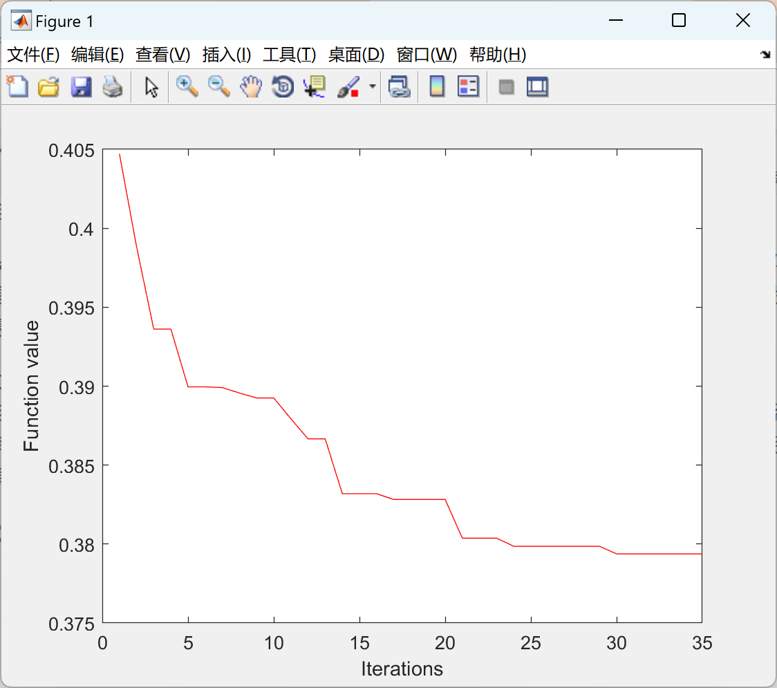
figure (1)
plot(bsof,'r'); xlabel('Iterations'); ylabel('Function value')
figure (2)
title('Voltage profile')
for k=1:n_nodosLim1(k)=0.95;Lim2(k)=1.05;
end
plot(V_o); hold on; plot(Vs); hold on; plot(Lim1,'--k'); hold on; plot(Lim2,'--k'); xlabel('# bus'); ylabel('Magnitude (pu)')
legend('Voltage base case','Voltage for the optimum solution')
figure (3)
title('Active power lossess')
y=[Plosses,Pls];
c=categorical({'Base case','Optimum solution'});
bar(c,y,'FaceColor',[0 .5 .5],'EdgeColor',[0 .9 .9],'LineWidth',1.5)
ylabel('Total active power lossess (pu)')
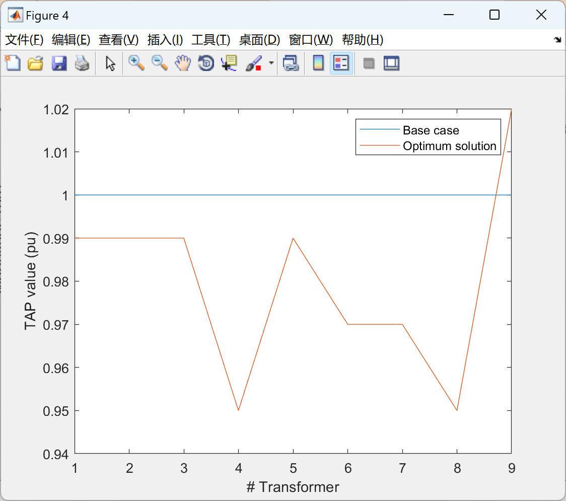
figure (4)
title('TAP values comparison')
plot(tap_o); hold on; plot(xitap(end,:)); xlabel('# Transformer'); ylabel('TAP value (pu)')
legend('Base case','Optimum solution')%+++++++++++++++++++ Data base of the power system ++++++++++++++++++++++++
% The following file contains information about the topology of the power
% system such as the bus and line matrix
data_39;
% original matrix and generation buses
bus_o=bus; line_o=line;
slack=find(bus(:,10)==1); % Slack bus
PV=find(bus(:,10)==2); % Generation buses PV
Bgen=vertcat(slack,PV); % Slack and PV buses
PQ=find(bus(:,10)==3); % Load buses
% +++++++++++++++ Parameters of the optimization algorithm ++++++++++++++++
pop = 210; % Size of the population
n_itera = 35; % Number of iterations of the optimization algorithm
Vmin=0.95; % Minimum value of voltage for the generators
Vmax=1.05; % Maximum value of voltage for the generators
mini_tap = 0.95; % Minimum value of the TAP
maxi_tap = 1.05; % Maximum value of the TAP
Smin=-0.5; % Minimum Shunt value
Smax=0.5; % Maximum Sunt value
pos_Shunt = find( bus(:,11) ~= 0); % Positions of Shunts in bus matrix
pos_tap = find( line(:,6) ~= 0); % Positions of TAPs in line matrix
tap_o = line(pos_tap,6); % Original values of TAPs
Shunt_o = bus(pos_Shunt,9); % Original values of Shunts
n_tap = length(pos_tap); % number of TAPs
n_Shunt = length(pos_Shunt); % number of Shunts
n_nodos = length(bus(:,1)); % number of buses of the power system
% ++++++++++++++++ First: Run power flow for the base case ++++++++++++++++
% Store V and theta of the base case
[V_o,Theta_o,~] = PowerFlowClassical(bus_o,line_o);
% +++++++++++++++++++Compute the active power lossess++++++++++++++++++++++
nbranch=length(line_o(:,1));
FromNode=line_o(:,1);
ToNode=line_o(:,2);
for k=1:nbranch
a(k)=line_o(k,6);
if a(k)==0 % in this case, we are analyzing lines
Zpq(k)=line_o(k,3)+1i*line_o(k,4); % impedance of the transmission line
Ypq(k)=Zpq(k)^-1; % admittance of the transmission linee
gpq(k)=real(Ypq(k)); % conductance of the transmission line
% Active power loss of the corresponding line
Llpq(k)=gpq(k)*(V_o(FromNode(k))^2 +V_o(ToNode(k))^2 -2*V_o(FromNode(k))*V_o(ToNode(k))*cos(Theta_o(FromNode(k))-Theta_o(ToNode(k))));
end
end
% Total active power lossess
Plosses=sum(Llpq);
% +++++++++++++++++++++++++++ Optimum power flow ++++++++++++++++++++++++++
% Start the population
for k=1:n_tap % Start the TAP population
x_tap(:,k) = mini_tap +(maxi_tap - mini_tap)*(0.1*floor((10*rand(pop,1))));
end
for k=1:n_Shunt % Start the Shunt population
x_shunt(:,k) = Smin +(Smax - Smin)*(0.1*floor((10*rand(pop,1))));
end
for k=1:length(Bgen) % Start the population of voltage from generators
x_vg(:,k) = Vmin +(Vmax - Vmin)*(0.1*floor((10*rand(pop,1))));
end
% JAYA algorithm
for k=1:n_itera
% with the new values of the TAPs, Shunts and VGs recompute V and Ybus
% Modify line and bus matrix
for p=1:pop
for q=1:n_tap
r=pos_tap(q);
line(r,6)=x_tap(p,q); % modification of line matrix acording to the new TAP values
end; clear r
for qa=1:n_Shunt
r=pos_Shunt(qa);
bus(r,9)=x_shunt(p,qa); % modification of bus matrix according to the new Shunt values
end; clear r
for qb=1:length(Bgen)
r=Bgen(qb);
bus(r,2)=x_vg(p,qb); % modification of bus matrix according to the new VG values
end
% With the new line and bus matrix run power flow
[V_n,Theta_n,~] = PowerFlowClassical(bus,line);
% Objective function
[F,~] = ObjectiveFunction(V_n,line_o,Bgen,Theta_n,nbranch,FromNode,ToNode,PQ);
Ofun=F; Obfun(k,p)=F;
end
% Define the new values of the desition variables: VGs, TAPs and Shunts
[x1,x2,x3] = UpdateDesitionVariables(Obfun(k,:),x_tap,x_shunt,x_vg);
% In this section, correct the particles that are surpassing the
% minimum/ maximum established values
% TAP values
xselect=round(100*x1); %discretize TAP values
x1=xselect/100;
x1a=x1;
for p=1:n_tap
for i=1:pop
if x1(i,p)<mini_tap
x1a(i,p)=mini_tap;
end
if x1(i,p)>maxi_tap
x1a(i,p)=maxi_tap;
end
end
end
% Shunt elements
x2a=x2;
for p=1:n_Shunt
for i=1:pop
if x2(i,p)<Smin
x2a(i,p)=Smin;
end
if x2(i,p)>Smax
x2a(i,p)=Smax;
end
end
end
% Voltages from generators
x3a=x3;
for p=1:length(Bgen)
for i=1:pop
if x3(i,p)<Vmin
x3a(i,p)=Vmin;
end
if x3(i,p)>Vmax
x3a(i,p)=Vmax;
end
end
end
x_tap=x1a; x_shunt=x2a; x_vg=x3a;
% With the corrected updated values, modify bus and line matrix
for p=1:pop
for q=1:n_tap
r=pos_tap(q);
line(r,6)=x_tap(p,q); % modification of line matrix acording to the new corrected TAP values
end; clear r
for qa=1:n_Shunt
r=pos_Shunt(qa);
bus(r,9)=x_shunt(p,qa); % modification of bus matrix according to the new corrected Shunt values
end; clear r
for qb=1:length(Bgen)
r=Bgen(qb);
bus(r,2)=x_vg(p,qb); % modification of bus matrix according to the new corrected VG values
end
% Run Newton Raphson
[V_n,Theta_n,~] = PowerFlowClassical(bus,line);
% Objective function
[Fnew,~] = ObjectiveFunction(V_n,line,Bgen,Theta_n,nbranch,FromNode,ToNode,PQ);
Obfunnew(k,p)=Fnew;
end
% Store values of TAPS, SHUNTS AND VGS for every iteration
XTAP(k,:,:)=x1a; XSHUNT(k,:,:)=x2a; XVG(k,:,:)=x3a;
if k>1
for i=1:pop
if(Obfunnew(k-1,i)<Obfunnew(k,i))
x_tap(i,:)=XTAP(k-1,i,:); x_shunt(i,:)=XSHUNT(k-1,i,:); x_vg(i,:)=XVG(k-1,i,:);
Obfunnew(k,i)=Obfunnew(k-1,i);
% In case that we needed the values of the previos iterations,
% we will have to change the storing matrix XTAP XSHUNT and XVG
XTAP(k,i,:)=x_tap(i,:); XSHUNT(k,i,:)=x_shunt(i,:); XVG(k,i,:)=x_vg(i,:);
end
end
end
% best solution at each iteration
bsof(k)=min(Obfunnew(k,:));
% Find the values of TAPs, Shunts and VGs associated to the best solution
for i=1:pop
if bsof(k)==Obfunnew(k,i)
xitap(k,:)=x_tap(i,:); % TAP values associate to the best solution
xishunt(k,:)=x_shunt(i,:); % Shunt values associate to the best solution
xivg(k,:)=x_vg(i,:); % VG values associate to the best solution
end
end
end
% ++++++++++++++++++++++++++++++++++Solution ++++++++++++++++++++++++++++++
% once the optimization algorithm has sttoped, run power flow with the
% solutions provided
% First, we modify line and bus
for q=1:n_tap
r=pos_tap(q);
line(r,6)=xitap(end,q); % modification of line matrix acording to the new corrected TAP values
end; clear r
for qa=1:n_Shunt
r=pos_Shunt(qa);
bus(r,9)=xishunt(end,qa); % modification of bus matrix according to the new corrected Shunt values
end; clear r
for qb=1:length(Bgen)
r=Bgen(qb);
bus(r,2)=xivg(end,qb); % modification of bus matrix according to the new corrected VG values
end
[Vs,Thetas,~] = PowerFlowClassical(bus,line);
[Fobjective,Pls] = ObjectiveFunction(Vs,line,Bgen,Thetas,nbranch,FromNode,ToNode,PQ);
% ++++++++++++++++++++++++++++++ Print results ++++++++++++++++++++++++++++
disp('OPTIMIZACI覰 MEDIANTE ALGORITMO JAYA')
disp(' ')
disp(' ')
disp(' VOLTAGE ANGLE ')
disp(' ----------------- ---------------- ')
disp(' BUS Orig JAYA Orig JAYA ')
disp(' ')
display_1=[bus(:,1) V_o Vs Theta_o*(180/pi) Thetas*(180/pi)];
disp(display_1)
figure (1)
plot(bsof,'r'); xlabel('Iterations'); ylabel('Function value')
figure (2)
title('Voltage profile')
for k=1:n_nodos
Lim1(k)=0.95;
Lim2(k)=1.05;
end
plot(V_o); hold on; plot(Vs); hold on; plot(Lim1,'--k'); hold on; plot(Lim2,'--k'); xlabel('# bus'); ylabel('Magnitude (pu)')
legend('Voltage base case','Voltage for the optimum solution')
figure (3)
title('Active power lossess')
y=[Plosses,Pls];
c=categorical({'Base case','Optimum solution'});
bar(c,y,'FaceColor',[0 .5 .5],'EdgeColor',[0 .9 .9],'LineWidth',1.5)
ylabel('Total active power lossess (pu)')
figure (4)
title('TAP values comparison')
plot(tap_o); hold on; plot(xitap(end,:)); xlabel('# Transformer'); ylabel('TAP value (pu)')
legend('Base case','Optimum solution')
🎉3 参考文献
文章中一些内容引自网络,会注明出处或引用为参考文献,难免有未尽之处,如有不妥,请随时联系删除。
[1]李璇.基于遗传算法的电力系统最优潮流问题研究[D].华中科技大学,2007.
[2]尤金.基于Jaya算法的DG优化配置研究[D].天津大学,2018.
[3]蒋承刚,熊国江,帅茂杭.基于DE-Jaya混合优化算法的电力系统经济调度方法[J].传感器与微系统, 2023.
🌈4 Matlab代码实现
相关文章:
基于Jaya优化算法的电力系统最优潮流研究(Matlab代码实现)
💥💥💞💞欢迎来到本博客❤️❤️💥💥 🏆博主优势:🌞🌞🌞博客内容尽量做到思维缜密,逻辑清晰,为了方便读者。 ⛳️座右铭&a…...

Write-Ahead Log(PostgreSQL 14 Internals翻译版)
日志 如果发生停电、操作系统错误或数据库服务器崩溃等故障,RAM中的所有内容都将丢失;只有写入磁盘的数据才会被保留。要在故障后启动服务器,必须恢复数据一致性。如果磁盘本身已损坏,则必须通过备份恢复来解决相同的问题。 理论…...
CUDA 学习记录
1.关于volatile: 对于文章中这个函数, __global__ void reduceUnrollWarps8 (int *g_idata, int *g_odata, unsigned int n) {// set thread IDunsigned int tid threadIdx.x;unsigned int idx blockIdx.x * blockDim.x * 8 threadIdx.x;// convert…...

【Java 进阶篇】深入了解 Bootstrap 按钮和图标
按钮和图标在网页设计中扮演着重要的角色,它们是用户与网站或应用程序交互的关键元素之一。Bootstrap 是一个流行的前端框架,提供了丰富的按钮样式和图标库,使开发者能够轻松创建吸引人的界面。在本文中,我们将深入探讨 Bootstrap…...

基于Java的人事管理系统设计与实现(源码+lw+部署文档+讲解等)
文章目录 前言具体实现截图论文参考详细视频演示为什么选择我自己的网站自己的小程序(小蔡coding) 代码参考数据库参考源码获取 前言 💗博主介绍:✌全网粉丝10W,CSDN特邀作者、博客专家、CSDN新星计划导师、全栈领域优质创作者&am…...

代码随想录算法训练营第五十九天| 647. 回文子串 516.最长回文子序列
今日学习的文章链接和视频链接 回文子串 https://programmercarl.com/0647.%E5%9B%9E%E6%96%87%E5%AD%90%E4%B8%B2.html 516.最长回文子序列 https://programmercarl.com/0516.%E6%9C%80%E9%95%BF%E5%9B%9E%E6%96%87%E5%AD%90%E5%BA%8F%E5%88%97.html 动态规划总结篇 https:…...

uniapp 小程序优惠劵样式
先看效果图 上代码 <view class"coupon"><view class"tickets" v-for"(item,index) in 10" :key"item"><view class"l-tickets"><view class"name">10元优惠劵</view><view cl…...

元梦之星内测上线,如何在B站打响声量?
元梦之星是腾讯天美工作室群研发的超开星乐园派对手游,于2023年1月17日通过审批。该游戏风格可爱软萌,带有社交属性,又是一款开黑聚会的手游,备受年轻人关注。 飞瓜数据(B站版)显示,元梦之星在…...
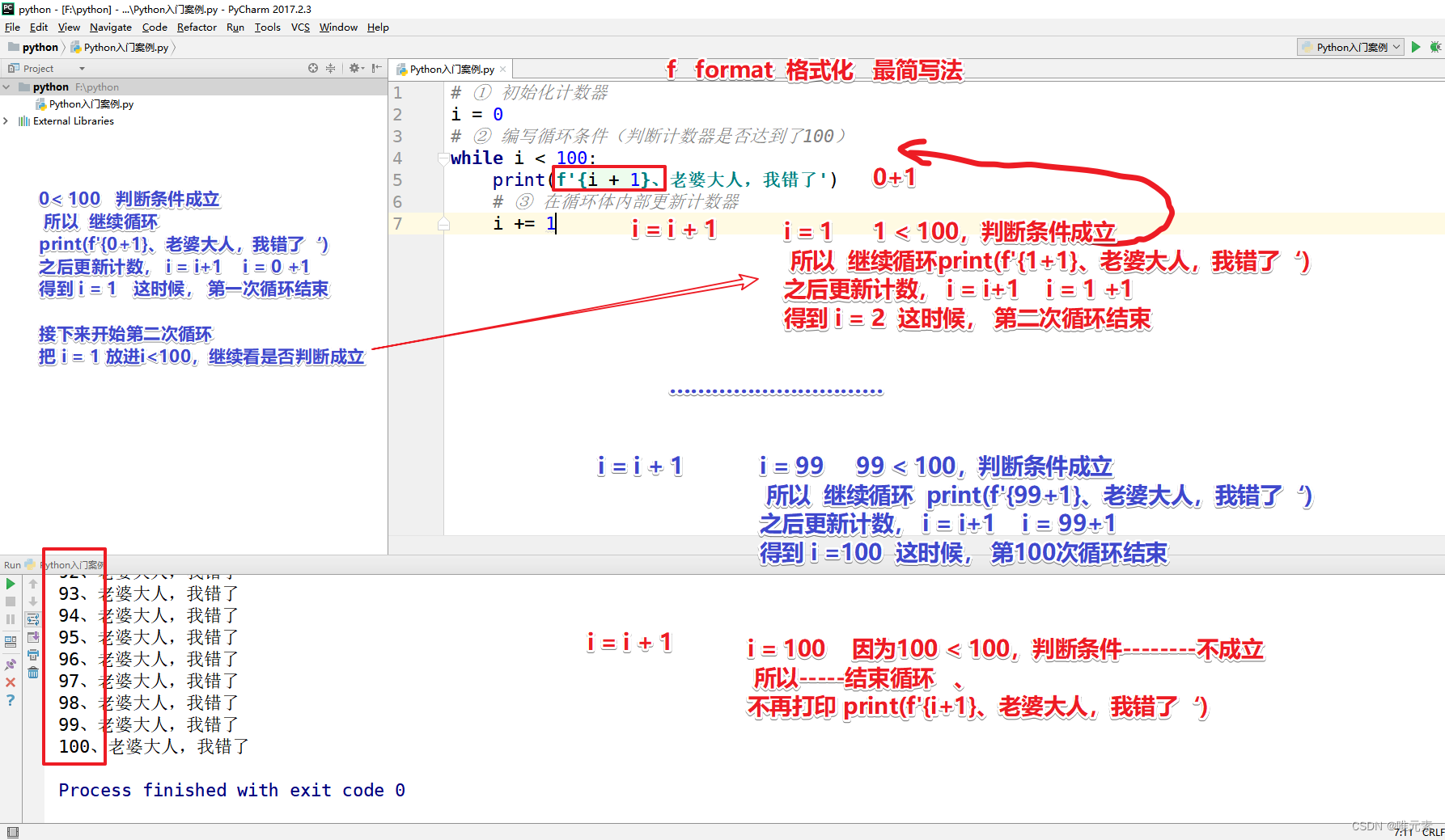
Python---循环---while循环
Python中的循环 包括 while循环与for循环,本文以while循环为主。 Python中所有的知识点,都是为了解决某个问题诞生的,就好比中文的汉字,每个汉字都是为了解决某种意思表达而诞生的。 1、什么是循环 现实生活中,也有…...

面试知识点--基础篇
文章目录 前言一、排序1. 冒泡排序2. 选择排序3. 插入排序4. 快速单边循环排序5. 快速双边循环排序6. 二分查找 二、集合1.List2.Map 前言 提示:以下是本篇文章正文内容,下面案例可供参考 一、排序 1. 冒泡排序 冒泡排序就是把小的元素往前调或者把大…...
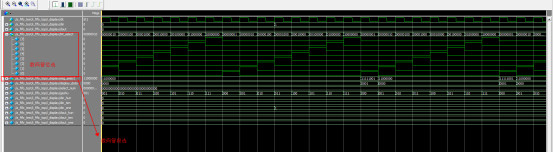
FIFO设计16*8,verilog,源码和视频
名称:FIFO设计16*8,数据显示在数码管 软件:Quartus 语言:Verilog 代码功能: 使用verilog语言设计一个16*8的FIFO,深度16,宽度为8。可对FIFO进行写和读,并将FIFO读出的数据显示到…...

#力扣:2769. 找出最大的可达成数字@FDDLC
2769. 找出最大的可达成数字 - 力扣(LeetCode) 一、Java class Solution {public int theMaximumAchievableX(int num, int t) {return num 2*t;} }...
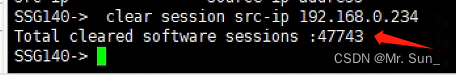
Juniper防火墙SSG-140 session 过高问题
1.SSG-140性能参数 2.问题截图 3.解决方法 (1)通过telnet 或 consol的方法登录到防火墙; (2)使用get session 查看总的session会话数,如果大于300 一般属于不正常情况 (3)使用get…...

Spring Boot 3.2四个新特点提升运行性能
随着 Spring Framework 6.1 和 Spring Boot 3.2 普遍可用性的临近,我们想分享一下 Spring 团队为让开发人员优化其应用程序的运行时效率而做出的几项努力的概述。 我们将介绍以下技术和用例: Spring MVC 将使用 基于JDK 21 虚拟线程 Web 堆栈使用 Spri…...

一阶系统阶跃响应实现规划方波目标值
一阶系统单位阶跃响应 一阶系统传递函数,实质是一阶惯性环节,T为一阶系统时间常数。 输入信号为单位阶跃函数,数学表达式 单位阶跃函数拉氏变换 输出一阶系统单位阶跃响应 拉普拉斯反变换 使用前向差分法对一阶系统离散化 将z变换写成差分方…...

项目经理如何去拆分复杂项目?
代码的横向分层,维度是根据复杂度来的,可保证代码便于开发和维护 1、因为强类型的原因,把变动大的分到数据库来解决,这是一种后端分离。 2、因为发布难的原因,所以用稳定的引擎来解决问题,然后用数据库配置…...
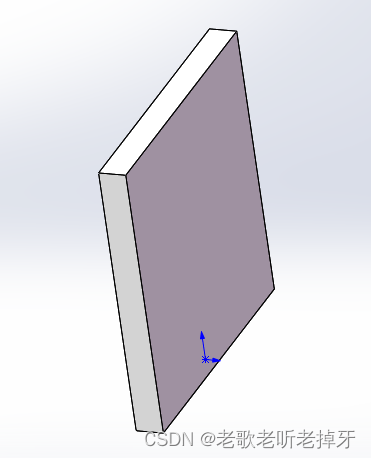
python二次开发Solidworks:修改实体尺寸
立方体原始尺寸:100mm100mm100mm 修改后尺寸:10mm100mm100mm import win32com.client as win32 import pythoncomdef bin_width(width):myDimension Part.Parameter("D1草图1")myDimension.SystemValue width def bin_length(length):myDime…...
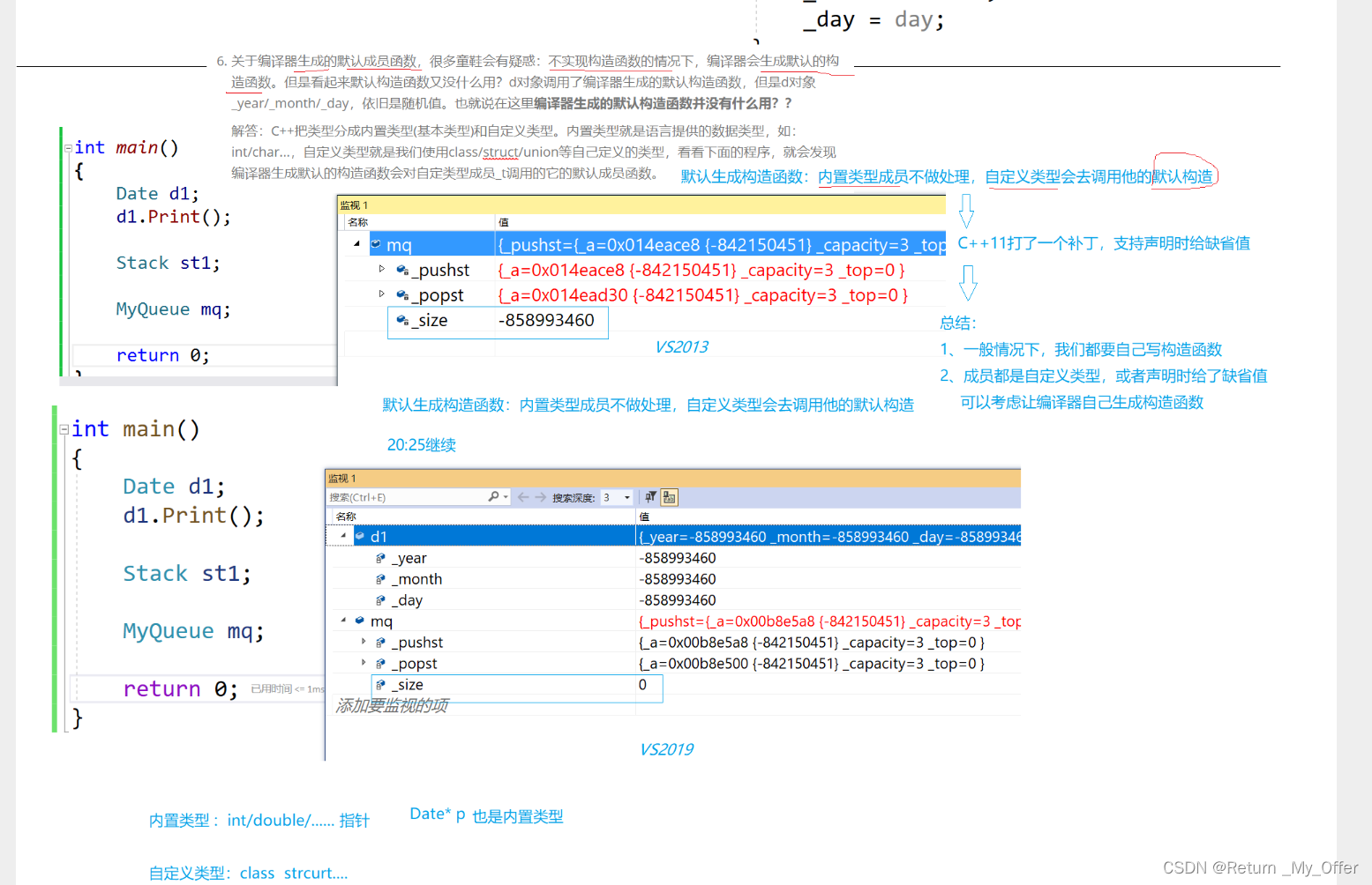
【C++】:类和对象(中)之类的默认成员函数——构造函数and析构函数
1.类的6个默认成员函数 如果一个类中什么成员都没有,简称为空类 空类中真的什么都没有吗?并不是,任何类在什么都不写时,编译器会自动生成以下6个默认成员函数 默认成员函数:用户没有显式实现,编译器会生成…...
sqlserver系统存储过程添加用户学习
sqlserver有一个系统存储过程sp_adduser;从名字看是添加用户的;操作一下, 从错误提示看还需要先添加一个登录名,再执行一个系统过程sp_addlogin看一下, 执行完之后看一下,安全性-登录名下面有了rabbit&…...

Monocle 3 | 太牛了!单细胞必学R包!~(一)(预处理与降维聚类)
1写在前面 忙碌的一周结束了,终于迎来周末了。🫠 这周的手术真的是做到崩溃,2天的手术都过点了。🫠 真的希望有时间静下来思考一下。🫠 最近的教程可能会陆续写一下Monocle 3,炙手可热啊,欢迎大…...

NaViL-9B多场景应用:法律合同截图理解+条款要点提取实战案例
NaViL-9B多场景应用:法律合同截图理解条款要点提取实战案例 1. 引言:当AI遇上法律合同 想象一下这样的场景:你刚收到一份20页的PDF合同,需要快速找出关键条款。传统方法是逐页阅读、手动标注,耗时又容易遗漏重点。现…...

工业级Wi-Fi 7接入点EKI-6333BE-4GD技术解析与应用
1. 工业级Wi-Fi 7接入点EKI-6333BE-4GD深度解析在工业自动化和机器人技术快速发展的今天,稳定可靠的无线网络连接已成为关键基础设施。研华科技(Advantech)最新推出的EKI-6333BE-4GD工业级Wi-Fi 7接入点,正是为满足这一需求而设计…...

Learning to AutoFocus:深度学习驱动的自动对焦实战
文章目录 Learning to AutoFocus:深度学习驱动的自动对焦实战 一、问题背景 二、技术方案 三、数据准备 四、模型 五、训练 六、推理与对焦控制 七、部署考虑 八、实验结果 九、总结 代码链接与详细流程 购买即可解锁1000+YOLO优化文章,并且还有海量深度学习复现项目,价格仅…...

OpenClaw System Prompt 构建流程学习笔记
OpenClaw System Prompt 构建流程学习笔记 概述 本笔记详细记录了 OpenClaw 如何将 AGENTS.md 文件内容动态注入到 LLM 的 system 提示词中的完整调用链。该机制是 OpenClaw 工程化设计的核心:用户通过文件系统配置系统行为,而非硬编码。 ✅ 核心结论:AGENTS.md 的内容以原…...

从惠斯通电桥到非平衡电桥:用FQJ型实验箱搞定Cu50和MF51温度传感器标定
从惠斯通电桥到非平衡电桥:用FQJ型实验箱搞定Cu50和MF51温度传感器标定 在温控系统开发中,传感器标定是决定测量精度的关键环节。传统实验室教学常将电桥实验局限于理论验证,而本文将展示如何将FQJ型非平衡电桥实验箱转化为工程实践工具&…...

GDB 调试完全指南:从入门到工程实战
GDB 调试完全指南:从入门到工程实战 这份教程旨在帮助你建立系统的调试思维,不仅掌握命令,更掌握解决复杂问题的方法。第一章:工欲善其事(环境与配置) 在开始调试之前,必须确保你的“武器”已经…...

开源代码审计工具opencode:基于异常检测的智能安全扫描实践
1. 项目概述:一个开源代码审计与异常检测工具最近在跟几个做安全开发的朋友聊天,大家普遍提到一个痛点:项目大了,代码库动辄几十万行,每次上线前的人工代码审计(Code Review)都像大海捞针&#…...

電機方向資料整理
1. 基本知識確認電機的接綫2.SVPWM2.1 svpwm是什么SVPWM(空间矢量脉宽调制)是一种用于三相电压源逆变器的调制技术。核心思想:把逆变器的 8 种开关状态看成空间中的 8 个基本电压矢量(6 个有效矢量,2 个零矢量…...
)
VS Code Copilot Next 配置实战手册(企业级自动化工作流搭建全流程)
更多请点击: https://intelliparadigm.com 第一章:VS Code Copilot Next 自动化工作流配置概览 VS Code Copilot Next 是微软与 GitHub 联合推出的下一代智能编程助手,它深度集成于 VS Code 编辑器中,支持上下文感知的代码生成、…...

面试官亲述:一道“发红包”用例设计题,我凭什么给他通过?
上周帮部门做校招面试,最近面试了不少校招同学,简历都挺能打——自动化框架、接口测试、性能压测都写着,项目经历至少两三个。我问了一个问题:“如果让你测试微信发红包,你怎么设计测试用例?”7个人里面&am…...