GEO生信数据挖掘(九)WGCNA分析
第六节,我们使用结核病基因数据,做了一个数据预处理的实操案例。例子中结核类型,包括结核,潜隐进展,对照和潜隐,四个类别。第七节延续上个数据,进行了差异分析。 第八节对差异基因进行富集分析。本节进行WGCNA分析。
更新版本:GEO生信数据挖掘(九)肺结核数据-差异分析-WGCNA分析(900行代码整理注释更新版本)
目录
加载数据,进行聚类
初次聚类观察
自己定义红线位置,进行切割划分
载入性状数据
增加形状信息后,再次聚类
网络构建
选取soft-thresholding powers
基于tom的差异的基因聚类,绘制聚类树
根据聚类情况,设置颜色
计算eigengenes
模块的自动合并
模块与临床形状的关系热图 (关键数据)
红色模块样本表达情况(相关性大)
产生了很多数据(各个模块的和临床性状)
后续挖掘核心基因时,需要用到Cytoscape,生成绘图所需要的数据
加载数据,进行聚类
library(WGCNA)
#读取目录名称,方便复制粘贴
dir()
#加载数据
load('DEG_TB_LTBI_step13.Rdata')#这里行为样品名,列为基因名
################################样品聚类####################
datExpr = t(dataset_TB_LTBI_DEG)
#初次聚类
sampleTree = hclust(dist(datExpr), method = "average")
# Plot the sample tree: Open a graphic output window of size 20 by 15 inches
# The user should change the dimensions if the window is too large or too small.
sizeGrWindow(12,9)
#pdf(file='sampleCluestering.pdf',width = 12,height = 9)
par(cex=0.6)
par(mar=c(0,4,2,0))
plot(sampleTree, main = "Sample clustering to detect outliers", sub="", xlab="", cex.lab = 1.5,cex.axis = 1.5, cex.main = 2)#结果图片自己导出PDF,文件名=1_sampleClustering.pdf### Plot a line to show the cut
abline(h = 87, col = "red")##剪切高度不确定,故无红线dev.off()
初次聚类观察

自己定义红线位置,进行切割划分
本例发现右侧有些样本孤立,适合被剔除,设置红线87切割。
左侧也被切成两块,需要做处理,保留。
### Determine cluster under the line
clust = cutreeStatic(sampleTree, cutHeight = 87, minSize = 10)
table(clust)
#clust
#0  1  2
#5 57 40### clust 1 contains the samples we want to keep.
keepSamples = (clust==1|clust==2)
datExpr0 = datExpr[keepSamples, ]
dim(datExpr0) #[1]   97 2813
#保存数据
save(datExpr0,file='datExpr0_cluster_filter.Rdata')
载入性状数据
匹配样本名称,性状数据与表达数据保证一致
#################### 载入性状数据###########################
#加载自己的性状数据
load('design_TB_LTBI.Rdata')
traitData=design
#Loading clinical trait data
#traitData = read.table("trait_D.txt",row.names=1,header=T,comment.char = "",check.names=F)########trait file name can be changed######性状数据文件名,根据实际修改,如果工作路径不是实际性状数据路径,需要添加正确的数据路径
dim(traitData)
#names(traitData)
# remove columns that hold information we do not need.
#allTraits = traitData
dim(traitData)
names(traitData)# Form a data frame analogous to expression data that will hold the clinical traits.
fpkmSamples = rownames(datExpr0)
traitSamples =rownames(traitData)
#匹配样本名称,性状数据与表达数据保证一致
traitRows = match(fpkmSamples, traitSamples)
datTraits = traitData[traitRows,]
rownames(datTraits)
collectGarbage()
增加形状信息后,再次聚类
# Re-cluster samples
sampleTree2 = hclust(dist(datExpr0), method = "average")
# Convert traits to a color representation: white means low, red means high, grey means missing entry
traitColors = numbers2colors(datTraits, signed = FALSE)
# Plot the sample dendrogram and the colors underneath.#sizeGrWindow(20,20)
##pdf(file="2_Sample dendrogram and trait heatmap.pdf",width=12,height=12)
plotDendroAndColors(sampleTree2, traitColors,groupLabels = names(datTraits),main = "Sample dendrogram and trait heatmap")dev.off()
下方红色,大致分成了两类,效果不错。

网络构建
#############################network constr######################################### Allow multi-threading within WGCNA. At present this call is necessary.
# Any error here may be ignored but you may want to update WGCNA if you see one.
# Caution: skip this line if you run RStudio or other third-party R environments.
# See note above.
enableWGCNAThreads()# Choose a set of soft-thresholding powers
powers = c(1:15)# Call the network topology analysis function
sft = pickSoftThreshold(datExpr0, powerVector = powers, verbose = 5)# Plot the results:
sizeGrWindow(15, 9)
#pdf(file="3_Scale independence.pdf",width=9,height=5)
#pdf(file="Rplot03.pdf",width=9,height=5)
par(mfrow = c(1,2))
cex1 = 0.9
# Scale-free topology fit index as a function of the soft-thresholding power
plot(sft$fitIndices[,1], -sign(sft$fitIndices[,3])*sft$fitIndices[,2],xlab="Soft Threshold (power)",ylab="Scale Free Topology Model Fit,signed R^2",type="n",main = paste("Scale independence"));
text(sft$fitIndices[,1], -sign(sft$fitIndices[,3])*sft$fitIndices[,2],labels=powers,cex=cex1,col="red");
# this line corresponds to using an R^2 cut-off of h
abline(h=0.90,col="red")
# Mean connectivity as a function of the soft-thresholding power
plot(sft$fitIndices[,1], sft$fitIndices[,5],xlab="Soft Threshold (power)",ylab="Mean Connectivity", type="n",main = paste("Mean connectivity"))
text(sft$fitIndices[,1], sft$fitIndices[,5], labels=powers, cex=cex1,col="red")
dev.off()
选取soft-thresholding powers
测试阈值,注意观察,突破红线的附近时取值,下方代码时候的是自适应的方法选取 soft-thresholding powers

######chose the softPower
#datExpr0= datExpr0[,-1]
softPower =sft$powerEstimate
adjacency = adjacency(datExpr0, power = softPower)##### Turn adjacency into topological overlap
TOM = TOMsimilarity(adjacency);
dissTOM = 1-TOM# Call the hierarchical clustering function
geneTree = hclust(as.dist(dissTOM), method = "average");
# Plot the resulting clustering tree (dendrogram)#sizeGrWindow(12,9)
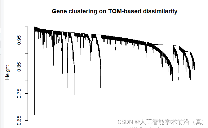
pdf(file="4_Gene clustering on TOM-based dissimilarity.pdf",width=12,height=9)
plot(geneTree, xlab="", sub="", main = "Gene clustering on TOM-based dissimilarity",labels = FALSE, hang = 0.04)
dev.off()基于tom的差异的基因聚类,绘制聚类树
根据聚类情况,设置颜色
# We like large modules, so we set the minimum module size relatively high:
minModuleSize = 30
# Module identification using dynamic tree cut:
dynamicMods = cutreeDynamic(dendro = geneTree, distM = dissTOM,deepSplit = 2, pamRespectsDendro = FALSE,minClusterSize = minModuleSize);
table(dynamicMods)# Convert numeric lables into colors
dynamicColors = labels2colors(dynamicMods)
table(dynamicColors)
# Plot the dendrogram and colors underneath
#sizeGrWindow(8,6)
pdf(file="5_Dynamic Tree Cut.pdf",width=8,height=6)
plotDendroAndColors(geneTree, dynamicColors, "Dynamic Tree Cut",dendroLabels = FALSE, hang = 0.03,addGuide = TRUE, guideHang = 0.05,main = "Gene dendrogram and module colors")
dev.off()

计算eigengenes
# Calculate eigengenes
MEList = moduleEigengenes(datExpr0, colors = dynamicColors)
MEs = MEList$eigengenes
# Calculate dissimilarity of module eigengenes
MEDiss = 1-cor(MEs);
# Cluster module eigengenes
METree = hclust(as.dist(MEDiss), method = "average")
# Plot the result
#sizeGrWindow(7, 6)
pdf(file="6_Clustering of module eigengenes.pdf",width=7,height=6)
plot(METree, main = "Clustering of module eigengenes",xlab = "", sub = "")
MEDissThres = 0.25######剪切高度可修改
# Plot the cut line into the dendrogram
abline(h=MEDissThres, col = "red")
dev.off()
模块的自动合并
# Call an automatic merging function
merge = mergeCloseModules(datExpr0, dynamicColors, cutHeight = MEDissThres, verbose = 3)
# The merged module colors
mergedColors = merge$colors
# Eigengenes of the new merged modules:
mergedMEs = merge$newMEs#sizeGrWindow(12, 9)
pdf(file="7_merged dynamic.pdf", width = 9, height = 6)
plotDendroAndColors(geneTree, cbind(dynamicColors, mergedColors),c("Dynamic Tree Cut", "Merged dynamic"),dendroLabels = FALSE, hang = 0.03,addGuide = TRUE, guideHang = 0.05)
dev.off()# Rename to moduleColors
moduleColors = mergedColors
# Construct numerical labels corresponding to the colors
colorOrder = c("grey", standardColors(50))
moduleLabels = match(moduleColors, colorOrder)-1
MEs = mergedMEs# Save module colors and labels for use in subsequent parts
save(MEs, TOM, dissTOM,  moduleLabels, moduleColors, geneTree, sft, file = "networkConstruction-stepByStep.RData")

模块与临床形状的关系热图 (关键数据)
#############################relate modules to external clinical triats######################################
# Define numbers of genes and samples
nGenes = ncol(datExpr0)
nSamples = nrow(datExpr0)moduleTraitCor = cor(MEs, datTraits, use = "p")
moduleTraitPvalue = corPvalueStudent(moduleTraitCor, nSamples)#sizeGrWindow(10,6)
pdf(file="8_Module-trait relationships.pdf",width=10,height=6)
# Will display correlations and their p-values
textMatrix = paste(signif(moduleTraitCor, 2), "\n(",signif(moduleTraitPvalue, 1), ")", sep = "")dim(textMatrix) = dim(moduleTraitCor)
par(mar = c(6, 8.5, 3, 3))# Display the correlation values within a heatmap plot #修改性状类型 data.frame
labeledHeatmap(Matrix = moduleTraitCor,xLabels = names(data.frame(datTraits)),yLabels = names(MEs),ySymbols = names(MEs),colorLabels = FALSE,colors = greenWhiteRed(50),textMatrix = textMatrix,setStdMargins = FALSE,cex.text = 0.5,zlim = c(-1,1),main = paste("Module-trait relationships"))
dev.off()
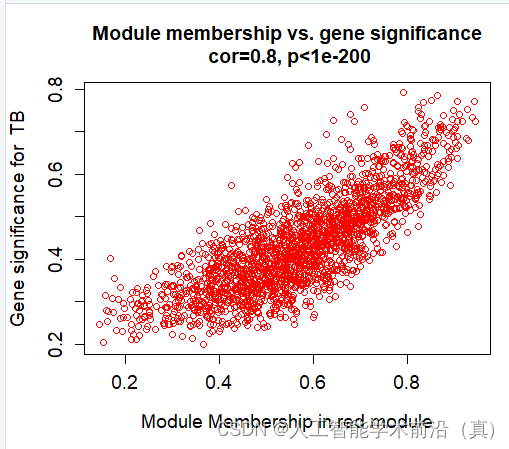
挑选相关性最高的,具有统计学意义的(p<0.05),red模块最佳!

红色模块样本表达情况(相关性大)
产生了很多数据(各个模块的和临床性状)
######## Define variable weight containing all column of datTraits###MM and GS# names (colors) of the modules
modNames = substring(names(MEs), 3)geneModuleMembership = as.data.frame(cor(datExpr0, MEs, use = "p"))
MMPvalue = as.data.frame(corPvalueStudent(as.matrix(geneModuleMembership), nSamples))names(geneModuleMembership) = paste("MM", modNames, sep="")
names(MMPvalue) = paste("p.MM", modNames, sep="")#names of those trait
traitNames=names(data.frame(datTraits))
class(datTraits)geneTraitSignificance = as.data.frame(cor(datExpr0, datTraits, use = "p"))
GSPvalue = as.data.frame(corPvalueStudent(as.matrix(geneTraitSignificance), nSamples))names(geneTraitSignificance) = paste("GS.", traitNames, sep="")
names(GSPvalue) = paste("p.GS.", traitNames, sep="")####plot MM vs GS for each trait vs each module##########example:royalblue and CK
module="red"
column = match(module, modNames)
moduleGenes = moduleColors==moduletrait="TB"
traitColumn=match(trait,traitNames)sizeGrWindow(7, 7)#par(mfrow = c(1,1))
verboseScatterplot(abs(geneModuleMembership[moduleGenes, column]),
abs(geneTraitSignificance[moduleGenes, traitColumn]),
xlab = paste("Module Membership in", module, "module"),
ylab = paste("Gene significance for ",trait),
main = paste("Module membership vs. gene significance\n"),
cex.main = 1.2, cex.lab = 1.2, cex.axis = 1.2, col = module)
######for (trait in traitNames){traitColumn=match(trait,traitNames)for (module in modNames){column = match(module, modNames)moduleGenes = moduleColors==moduleif (nrow(geneModuleMembership[moduleGenes,]) > 1){####进行这部分计算必须每个模块内基因数量大于2,由于前面设置了最小数量是30,这里可以不做这个判断,但是grey有可能会出现1个gene,它会导致代码运行的时候中断,故设置这一步#sizeGrWindow(7, 7)pdf(file=paste("9_", trait, "_", module,"_Module membership vs gene significance.pdf",sep=""),width=7,height=7)par(mfrow = c(1,1))verboseScatterplot(abs(geneModuleMembership[moduleGenes, column]),abs(geneTraitSignificance[moduleGenes, traitColumn]),xlab = paste("Module Membership in", module, "module"),ylab = paste("Gene significance for ",trait),main = paste("Module membership vs. gene significance\n"),cex.main = 1.2, cex.lab = 1.2, cex.axis = 1.2, col = module)dev.off()}}
}#####
names(datExpr0)
probes = names(datExpr0)#################export GS and MM############### geneInfo0 = data.frame(probes= probes,moduleColor = moduleColors)for (Tra in 1:ncol(geneTraitSignificance))
{oldNames = names(geneInfo0)geneInfo0 = data.frame(geneInfo0, geneTraitSignificance[,Tra],GSPvalue[, Tra])names(geneInfo0) = c(oldNames,names(geneTraitSignificance)[Tra],names(GSPvalue)[Tra])
}for (mod in 1:ncol(geneModuleMembership))
{oldNames = names(geneInfo0)geneInfo0 = data.frame(geneInfo0, geneModuleMembership[,mod],MMPvalue[, mod])names(geneInfo0) = c(oldNames,names(geneModuleMembership)[mod],names(MMPvalue)[mod])
}
geneOrder =order(geneInfo0$moduleColor)
geneInfo = geneInfo0[geneOrder, ]write.table(geneInfo, file = "10_GS_and_MM.xls",sep="\t",row.names=F)
####################################################Visualizing the gene network#######################################################nGenes = ncol(datExpr0)
nSamples = nrow(datExpr0)# Transform dissTOM with a power to make moderately strong connections more visible in the heatmap
plotTOM = dissTOM^7
# Set diagonal to NA for a nicer plot
diag(plotTOM) = NA# Call the plot functionsizeGrWindow(9,9) #这个耗电脑内存
pdf(file="12_Network heatmap plot_all gene.pdf",width=9, height=9)
TOMplot(plotTOM, geneTree, moduleColors, main = "Network heatmap plot, all genes")
dev.off()nSelect = 400
# For reproducibility, we set the random seed
set.seed(10)
select = sample(nGenes, size = nSelect)
selectTOM = dissTOM[select, select]
# There's no simple way of restricting a clustering tree to a subset of genes, so we must re-cluster.
selectTree = hclust(as.dist(selectTOM), method = "average")
selectColors = moduleColors[select]# Open a graphical window
#sizeGrWindow(9,9)
# Taking the dissimilarity to a power, say 10, makes the plot more informative by effectively changing
# the color palette; setting the diagonal to NA also improves the clarity of the plot
plotDiss = selectTOM^7
diag(plotDiss) = NApdf(file="13_Network heatmap plot_selected genes.pdf",width=9, height=9)
TOMplot(plotDiss, selectTree, selectColors, main = "Network heatmap plot, selected genes")
dev.off()####################################################Visualizing the gene network of eigengenes#####################################################sizeGrWindow(5,7.5)
pdf(file="14_Eigengene dendrogram and Eigengene adjacency heatmap.pdf", width=5, height=7.5)
par(cex = 0.9)
plotEigengeneNetworks(MEs, "", marDendro = c(0,4,1,2), marHeatmap = c(3,4,1,2), cex.lab = 0.8, xLabelsAngle= 90)
dev.off()#or devide into two parts
# Plot the dendrogram
#sizeGrWindow(6,6);
pdf(file="15_Eigengene dendrogram_2.pdf",width=6, height=6)
par(cex = 1.0)
plotEigengeneNetworks(MEs, "Eigengene dendrogram", marDendro = c(0,4,2,0), plotHeatmaps = FALSE)
dev.off()pdf(file="15_Eigengene adjacency heatmap_2.pdf",width=6, height=6)
# Plot the heatmap matrix (note: this plot will overwrite the dendrogram plot)
par(cex = 1.0)
plotEigengeneNetworks(MEs, "Eigengene adjacency heatmap", marHeatmap = c(3,4,2,2), plotDendrograms = FALSE, xLabelsAngle = 90)
dev.off()后续挖掘核心基因时,需要用到Cytoscape,生成绘图所需要的数据
###########################Exporting to Cytoscape all one by one ########################### Select each module
'''
Error in exportNetworkToCytoscape(modTOM, edgeFile = paste("CytoscapeInput-edges-",  : Cannot determine node names: nodeNames is NULL and adjMat has no dimnames.datExpr0 格式需要dataframe
'''
modules =module
for (mod in 1:nrow(table(moduleColors)))
{modules = names(table(moduleColors))[mod]# Select module probesprobes = names(data.frame(datExpr0))  # inModule = (moduleColors == modules)modProbes = probes[inModule]modGenes = modProbes# Select the corresponding Topological OverlapmodTOM = TOM[inModule, inModule]dimnames(modTOM) = list(modProbes, modProbes)# Export the network into edge and node list files Cytoscape can readcyt = exportNetworkToCytoscape(modTOM,edgeFile = paste("CytoscapeInput-edges-", modules , ".txt", sep=""),nodeFile = paste("CytoscapeInput-nodes-", modules, ".txt", sep=""),weighted = TRUE,threshold = 0.02,nodeNames = modProbes,altNodeNames = modGenes,nodeAttr = moduleColors[inModule])
}
关系网络的构建完毕,绘图找核心基因,Cytoscape 到底怎么玩?
相关文章:
GEO生信数据挖掘(九)WGCNA分析
第六节,我们使用结核病基因数据,做了一个数据预处理的实操案例。例子中结核类型,包括结核,潜隐进展,对照和潜隐,四个类别。第七节延续上个数据,进行了差异分析。 第八节对差异基因进行富集分析。…...
)
Python 中,单例模式的5种实现方式(使用模块、使用装饰器、使用类方法、基于new方法实现、基于metaclass方式实现)
单例模式的5种实现方式 1 使用模块 2 使用装饰器 3 使用类方法 4.基于new方法实现 5 基于metaclass方式实现 单例模式的5种实现方式 什么是单例模式? 单例模式是指:保证一个类仅有一个实例,并提供一个访问它的全局访问点# 线程1 执行&#x…...

超低延迟直播技术路线,h265的无奈选择
超低延迟,多窗显示,自适应编解码和渲染,高分辨低码率,还有微信小程序的标配,这些在现今的监控和直播中都成刚需了,中国的音视频技术人面临着困境,核心门户浏览器不掌握在自己手上,老…...
openstack 云主机 linux报 login incorrect
还未输入密码就提示login incorrect 不给输密码位置 完全不给输密码的机会 关机进入单用户 检查登录安全记录 vi /var/log/secure 发现 /usr/lib64/security/pam_unix.so 报错 将正常的机器提取/usr/lib64/security/pam_unix.so 比对MD5一致, 另外判断 libtir…...

Selenium:Web自动化框架
Selenium自动化入门 1、Selenium概述2、Selenium环境搭建3、Selenium基本操作4、网页元素定位5、操作Cookie6、标签页管理 1、Selenium概述 Selenium(Web Browser Automation)的初衷是Web应用自动化测试。Selenium广泛应用于爬虫,爬虫需要让浏…...

Android11 添加adb后门
软件平台:Android11 硬件平台:QCS6125 需求:通过设备的物理组合按键,直接打开adb功能,我们这里确定的是Volume-up、Volume-down、camera三个按键在短时间内各按三次即可触发,具体代码改动如下:…...
福昕阅读器打开pdf文档时显示的标题不是文件名
0 Preface/Foreword 1 现象 文件名为:Demo-20231017 打开效果:显示名字为 word template 2 解决方法 2.1 利用打印方式将word生产pdf 在word生成pdf文件时,使用打印方式生成pdf文档。 2.2 删除word文档设置的标题 文件---》信息---》标…...

Python自创项目—《数字帝国》更新日志
Inscode项目地址:https://inscode.csdn.net/2302_76241188/lxzn 或者点这里访问 更新时间:2023-10-04 更新内容:新增加四个地区 附:预计下次更新将会增加几个新的地区,修复一些已知bug...
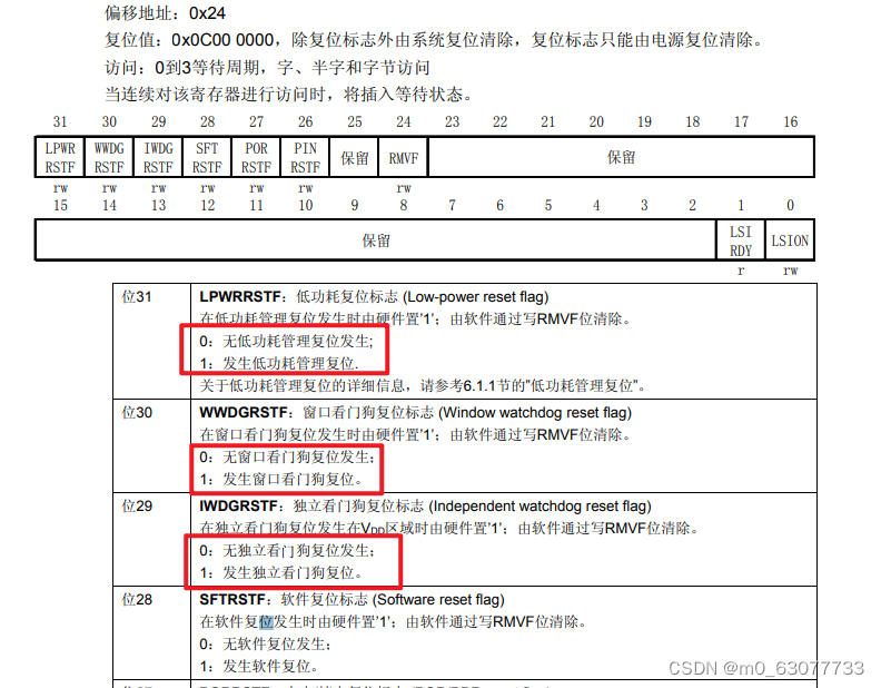
【STM32】---存储器,电源核时钟体系
一、STM32的存储器映像 1 文中的缩写 2 系统构架(原理图) 3. 存储器映像 (1)STM32是32位CPU,数据总线是32位的 (2)STM232的地址总线是32位的。(其实地址总线是32位不是由数据总线是…...

Flink中的时间和窗口操作
1.窗口概念 在大多数场景下,我们需要统计的数据流都是无界的,因此我们无法等待整个数据流终止后才进行统计。通常情况下,我们只需要对某个时间范围或者数量范围内的数据进行统计分析:如每隔五分钟统计一次过去一小时内所有商品的点击量;或者每发生1000次点击后,都去统计一…...

【算法|前缀和系列No.5】leetcode1314. 矩阵区域和
个人主页:兜里有颗棉花糖 欢迎 点赞👍 收藏✨ 留言✉ 加关注💓本文由 兜里有颗棉花糖 原创 收录于专栏【手撕算法系列专栏】【Leetcode】 🍔本专栏旨在提高自己算法能力的同时,记录一下自己的学习过程,希望…...

python知识:从PDF 提取文本
一、说明 PDF 到文本提取是自然语言处理和数据分析中的一项基本任务,它允许研究人员和数据分析师从 PDF 文件中包含的非结构化文本数据中获得见解。Python 是一种通用且广泛使用的编程语言,它提供了多个库和工具来促进提取过程。 二、各种PDF操作库 让我…...
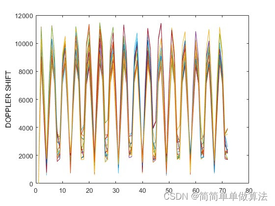
基于MATLAB的GPS卫星绕地运行轨迹动态模拟仿真
目录 1.算法运行效果图预览 2.算法运行软件版本 3.部分核心程序 4.算法理论概述 5.算法完整程序工程 1.算法运行效果图预览 2.算法运行软件版本 matlab2022a 3.部分核心程序 Prn NavData(PRNS_SEL,1);%识别导航数据中的PRNiode NavData(PRNS_SEL,11);%企…...

TCP/IP模型五层协议
TCP/IP模型五层协议 认识协议 约定双方进行的一种约定 协议分层 降低了学习和维护的成本(封装)灵活的针对这里的某一层协议进行替换 四/五层协议 五层协议的作用 应用层 应用层常见协议 应用层常见协议概览 基于TCP的协议 HTTP(超…...
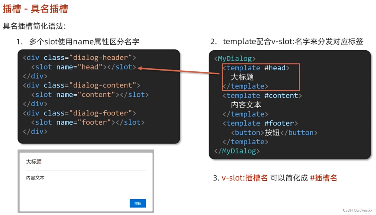
vue 插槽 - 具名插槽
vue 插槽 - 具名插槽 **创建 工程: H:\java_work\java_springboot\vue_study ctrl按住不放 右键 悬着 powershell H:\java_work\java_springboot\js_study\Vue2_3入门到实战-配套资料\01-随堂代码素材\day05\准备代码\09-插槽-具名插槽 vue --version vue create…...

Elasticsearch2.x Doc values
文档地址: https://www.elastic.co/guide/en/elasticsearch/reference/2.4/doc-values.html https://www.elastic.co/guide/en/elasticsearch/guide/2.x/docvalues-intro.html https://www.elastic.co/guide/en/elasticsearch/guide/2.x/docvalues.html https://ww…...
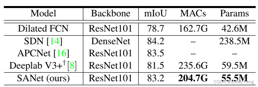
Squeeze-and-Attention Networks for Semantic Segmentation
0.摘要 最近,将注意力机制整合到分割网络中可以通过更重视提供更多信息的特征来提高它们的表征能力。然而,这些注意力机制忽视了语义分割的一个隐含子任务,并受到卷积核的网格结构的限制。在本文中,我们提出了一种新颖的squeeze-a…...
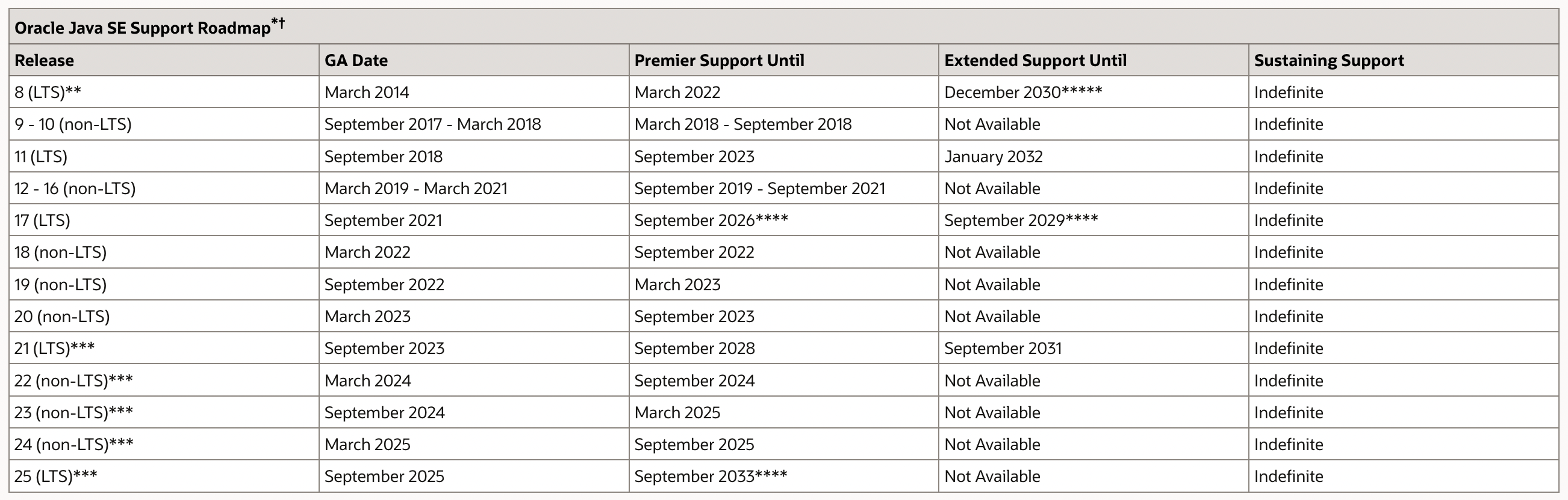
【Java】Java 11 新特性概览
Java 11 新特性概览 1. Java 11 简介2. Java 11 新特性2.1 HTTP Client 标准化2.2 String 新增方法(1)str.isBlank() - 判断字符串是否为空(2)str.lines() - 返回由行终止符划分的字符串集合(3)str.repeat(…...

用Vue3.0 写过组件吗?如果想实现一个 Modal你会怎么设计?
一、组件设计 组件就是把图形、非图形的各种逻辑均抽象为一个统一的概念(组件)来实现开发的模式 现在有一个场景,点击新增与编辑都弹框出来进行填写,功能上大同小异,可能只是标题内容或者是显示的主体内容稍微不同 …...
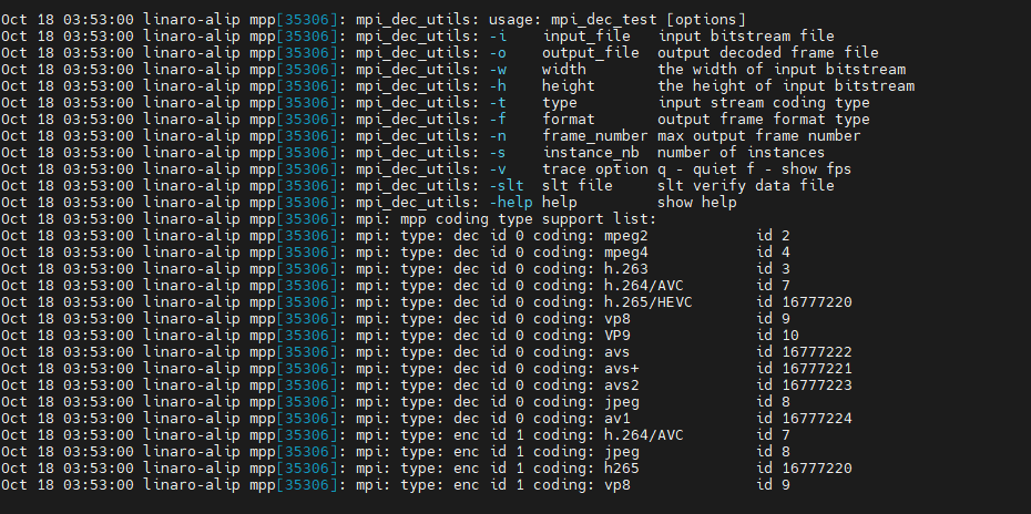
ArmSoM-W3之RK3588硬编解码MPP环境配置
1. 简介 瑞芯微提供的媒体处理软件平台(Media Process Platform,简称 MPP)是适用于瑞芯微芯片系列的 通用媒体处理软件平台。该平台对应用软件屏蔽了芯片相关的复杂底层处理,其目的是为了屏蔽不 同芯片的差异,为使用者…...

WarcraftHelper:魔兽争霸3性能优化与兼容性修复完全指南
WarcraftHelper:魔兽争霸3性能优化与兼容性修复完全指南 【免费下载链接】WarcraftHelper Warcraft III Helper , support 1.20e, 1.24e, 1.26a, 1.27a, 1.27b 项目地址: https://gitcode.com/gh_mirrors/wa/WarcraftHelper 还在为《魔兽争霸3》这款经典RTS游…...

陈、智能热板仪 大鼠热板仪 小鼠热板仪 大小鼠冷热板仪
热板法是镇痛药物筛选、区分中枢与外周镇痛机理的常用实验方法。传统实验温控、计时精度差,人为干扰大,数据重复性低。本仪器控温精准、计时精密,有效提升实验稳定性,适用于小鼠、大鼠、豚鼠镇痛检测实验。安徽,正华生…...

WinClaw:Go语言实现的Windows轻量级自动化库实战指南
1. 项目概述:一个Windows环境下的轻量级自动化利器最近在折腾一些Windows环境下的自动化任务,比如批量重命名文件、定时清理日志、自动整理桌面截图,或者是一些需要重复点击的简单GUI操作。一开始想着用Python写脚本,但涉及到UI自…...

使用Nodejs与Taotoken为你的Nextjs项目快速集成AI对话能力
使用 Node.js 与 Taotoken 为你的 Next.js 项目快速集成 AI 对话能力 1. 准备工作 在开始集成前,请确保已具备以下条件:一个可运行的 Next.js 项目(版本 12 或更高),以及 Taotoken 平台的 API Key。API Key 可在 Tao…...

PyCATIA:企业级CAD自动化解决方案与技术实现指南
PyCATIA:企业级CAD自动化解决方案与技术实现指南 【免费下载链接】pycatia python module for CATIA V5 automation 项目地址: https://gitcode.com/gh_mirrors/py/pycatia PyCATIA作为基于Python语言的CATIA V5/V6全栈式自动化模块,为制造企业提…...

KISSABC伴学 英语沉浸式伴学优势深度解析
KISSABC伴学聚焦少儿英语伴学,以“沉浸式语言环境专业引导”为核心,区别于传统英语学习工具“跟读式”“刷题式”的学习模式,打造“听、说、读、玩”四位一体的沉浸式伴学体验,助力孩子培养语感、规范发音、提升口语,贴…...
)
别再死记硬背了!用Python递归函数5分钟搞定二叉树前序/中序/后序转换(附PTA真题解析)
用Python递归思维破解二叉树遍历转换难题 第一次接触二叉树的前序、中序、后序遍历转换时,你是否也曾在各种递归调用和数组下标中迷失方向?作为数据结构学习路上的经典难题,这三种遍历方式的相互转换常常让初学者感到头疼。但今天我要分享的&…...

3种高效处理方案:如何优化AutoDock-Vina中金属离子电荷的技术实现
3种高效处理方案:如何优化AutoDock-Vina中金属离子电荷的技术实现 【免费下载链接】AutoDock-Vina AutoDock Vina 项目地址: https://gitcode.com/gh_mirrors/au/AutoDock-Vina 在分子对接研究中,金属离子配位体系的准确处理一直是计算药物发现的…...

KeymouseGo完整教程:免费开源鼠标键盘自动化工具终极指南
KeymouseGo完整教程:免费开源鼠标键盘自动化工具终极指南 【免费下载链接】KeymouseGo 类似按键精灵的鼠标键盘录制和自动化操作 模拟点击和键入 | automate mouse clicks and keyboard input 项目地址: https://gitcode.com/gh_mirrors/ke/KeymouseGo Keymo…...

从《Java编程思想》到《On Java 8》:开发者必须掌握的10个核心升级技巧
从《Java编程思想》到《On Java 8》:开发者必须掌握的10个核心升级技巧 【免费下载链接】OnJava8 《On Java 8》中文版 项目地址: https://gitcode.com/gh_mirrors/on/OnJava8 《On Java 8》作为《Java编程思想》的升级版,不仅延续了经典Java教程…...