【机器学习】从底层手写实现线性回归
【机器学习】Building-Linear-Regression-from-Scratch
- 线性回归 Linear Regression
- 0. 数据的导入与相关预处理
- 0.工具函数
- 1. 批量梯度下降法 Batch Gradient Descent
- 2. 小批量梯度下降法 Mini Batch Gradient Descent(在批量方面进行了改进)
- 3. 自适应梯度下降法 Adagrad(在学习率方面进行了改进)
- 4. 多变量线性回归 Multivariate Linear Regression(在特征方面进行了改进,拓展到多个特征)
- 5. L1正则化 L1 Regularization(在正则化方面进行了改进)
This project is not about using ready-made libraries; it’s an exploration into the core principles that power linear regression. We start from basic mathematics and progressively build up to a fully functioning linear regression model. This hands-on approach is designed for learners and enthusiasts who want to deeply understand the intricacies of one of the most fundamental algorithms in machine learning. Dive in to experience linear regression like never before!
这个项目不是关于使用现成的库,而是对驱动线性回归的核心原则的一次探索。我们从基础数学开始,逐步构建出一个功能完善的线性回归模型。这种实践方法专为那些希望深入理解机器学习中最基本算法之一的复杂性的学习者和爱好者设计。深入体验前所未有的线性回归!
If you find the code helpful, please give me a Star.
如果觉得代码对你有帮助,请给我一个Star.
前往Github下载notebook
https://github.com/Zhu-Shatong/Building-Linear-Regression-from-Scratch
线性回归 Linear Regression
CopyRight: Zhu Shatong , Tongji University
本notebook所有算法均为手写,不使用任何库函数。
(算法设计部分)目录:
- 准备工作:数据的导入与相关预处理,相关工具函数的定义
- (单变量线性回归的)批量梯度下降法 Batch Gradient Descent
- 小批量梯度下降法 Mini Batch Gradient Descent(在批量方面进行了改进)
- 自适应梯度下降法 Adagrad(在学习率方面进行了改进)
- 多变量线性回归 Multivariate Linear Regression(在特征方面进行了改进,拓展到多个特征)
- L1正则化 L1 Regularization(也就是Lasso Regression,应对多变量的过拟合)
0. 数据的导入与相关预处理
在这一section, 我们将会负责导入数据,并对数据进行一些预处理,以便于后续的操作。
data:
我们首先导入的文件为 data.xlsx ,将它存储在data变量中。这个文件中包含了两列数据,分别为 x 和 y 。
我们将会使用这些数据来进行线性回归的训练与可视化。
请注意,在后续本notebook中使用其他数据的时候,请勿再次命名为data。
数据来源:
Data on length-weight and length-length relationships, mean condition factor, and gonadosomatic index of Rutilus rutilus and Perca fluviatilis from the Ob River basin, Western Siberia - ScienceDirect
# 这一code block用来import需要的库import pandas as pd  # 用来读取excel等文件
import random  # 用来进行随机打乱数据
import numpy as np  # 用来进行矩阵运算,应对多变量线性回归
# 这一code block用来读取数据data = pd.read_excel("data.xlsx") # 读取excel文件(单变量线性回归——测试文件)
# 这一code block用来对读取的数据进行一些处理# 从数据框架中提取x和y值
x_values = data['x'].values
y_values = data['y'].values
0.工具函数
在这一section, 我们将会定义一些工具函数,以便于后续的操作。
目录:
- 可视化工具函数
- 线性回归模型计算
- 损失函数计算
# 可视化工具函数
# 对于数据点与拟合直线的可视化
def plot_data_and_line(x_values, y_values, theta_0_final, theta_1_final, cost_history, title):"""Plot data points and the fitted line.:param x_values: 这是一个list,包含了所有的x值:param y_values: 这是一个list,包含了所有的y值:param theta_0_final: 这是一个float,表示最终的theta_0:param theta_1_final: 这是一个float,表示最终的theta_1:param cost_history: 这是一个list,包含了每一次迭代后的损失函数值:param title: 这是一个string,表示图像的标题:return: 返回一个图像"""import matplotlib.pyplot as plt  # 用来画图plt.figure(figsize=(12, 5))# Subplot 1: Linear Regression# 这个subplot用来画出数据点和拟合直线plt.subplot(1, 2, 1)plt.scatter(x_values, y_values, color='blue', label='Original Data')  # 这里的scatter用来画出数据点plt.plot(x_values, [f_theta(x, theta_0_final, theta_1_final) for x in x_values], color='red',label='Linear Regression')  # 这里的列表表达式用来画出拟合直线plt.title(title)plt.xlabel('x')plt.ylabel('y')plt.legend()plt.grid(True)  # 显示网格# Subplot 2: Cost function history# 这个subplot用来画出损失函数的变化plt.subplot(1, 2, 2)plt.plot(cost_history, color='green')  # 这里的plot用来画出损失函数的变化plt.title('Cost Function History')plt.xlabel('Iteration')plt.ylabel('Cost')plt.grid(True)  # 显示网格plt.tight_layout()  # 调整子图之间的间距plt.show()
hypothesis:
f θ ( x ) = θ 0 + θ 1 x f_\theta(x)=\theta_0+\theta_1x fθ(x)=θ0+θ1x
def f_theta(x, theta_0, theta_1):"""Linear regression model.:param x: 这是一个float,表示输入的x值:param theta_0: 这是一个float,表示theta_0:param theta_1: 这是一个float,表示theta_1:return: 这是一个float,表示预测值"""return theta_0 + theta_1 * x
cost fuction:
J ( θ 0 , θ 1 ) = 1 2 N ∑ i = 1 N ( f θ ( x ( i ) ) − y ( i ) ) 2 J(\theta_0,\theta_1)=\frac1{2N}\sum_{i=1}^N(f_\theta(x^{(i)})-y^{(i)})^2 J(θ0,θ1)=2N1i=1∑N(fθ(x(i))−y(i))2
def compute_cost(x_values, y_values, theta_0, theta_1):"""Compute the cost function.:param x_values: 这是一个list,包含了所有的x值:param y_values: 这是一个list,包含了所有的y值:param theta_0: 这是一个float,表示theta_0:param theta_1: 这是一个float,表示theta_1:return: 这是一个float,表示损失函数的值"""# 计算的公式为:J(theta_0, theta_1) = 1/2N * sum((f_theta(x_i) - y_i)^2)N = len(x_values)total_error = 0for i in range(len(x_values)):total_error += (f_theta(x_values[i], theta_0, theta_1) - y_values[i]) ** 2return total_error / (2 * N)
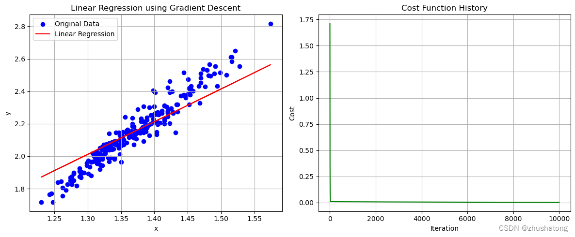
1. 批量梯度下降法 Batch Gradient Descent
repeat until convergence:
θ j : = θ j − α ∂ ∂ θ j J ( θ 0 , θ 1 ) ( for j = 1 and j = 0 ) \theta_j:=\theta_j-\alpha\frac{\partial}{\partial\theta_j}J(\theta_0,\theta_1) \\ (\text{for }j=1\text{ and }j=0) θj:=θj−α∂θj∂J(θ0,θ1)(for j=1 and j=0)
Repeat until convergence:
θ 0 : = θ 0 − a 1 N ∑ i = 1 N ( f θ ( x ( i ) ) − y ( i ) ) θ 1 : = θ 1 − a 1 N ∑ i = 1 N ( f θ ( x ( i ) ) − y ( i ) ) x ( i ) \begin{aligned}\theta_0{:}&=\theta_0-a\frac1N\sum_{i=1}^N(f_\theta\big(x^{(i)}\big)-y^{(i)})\\\theta_1{:}&=\theta_1-a\frac1N\sum_{i=1}^N(f_\theta\big(x^{(i)}\big)-y^{(i)})x^{(i)}\end{aligned} θ0:θ1:=θ0−aN1i=1∑N(fθ(x(i))−y(i))=θ1−aN1i=1∑N(fθ(x(i))−y(i))x(i)
def gradient_descent(x_values, y_values, alpha=0.05, convergence_threshold=1e-8, max_iterations=10000):"""Perform gradient descent to learn theta_0 and theta_1.:param x_values: 这是一个list,包含了所有的x值:param y_values: 这是一个list,包含了所有的y值:param alpha: 这是一个float,表示学习率:param convergence_threshold: 这是一个float,表示收敛阈值:param max_iterations: 这是一个int,表示最大迭代次数:return: 这是一个tuple,包含了theta_0, theta_1, cost_history,分别表示最终的theta_0, theta_1和损失函数的变化"""# 计算公式为: theta_j = theta_j - alpha * 1/N * sum((f_theta(x_i) - y_i) * x_i)theta_0 = 0 # 初始化theta_0theta_1 = 0 # 初始化theta_1N = len(x_values) # 样本数量cost_history = [] # 用来保存损失函数的变化for _ in range(max_iterations): # 进行迭代sum_theta_0 = 0 # 用来计算theta_0的梯度sum_theta_1 = 0 # 用来计算theta_1的梯度for i in range(N):error = f_theta(x_values[i], theta_0, theta_1) - y_values[i] # 计算误差sum_theta_0 += errorsum_theta_1 += error * x_values[i]# 注意,所有的theta的更新都是在同一时刻进行的theta_0 -= alpha * (1 / N) * sum_theta_0theta_1 -= alpha * (1 / N) * sum_theta_1cost_history.append(compute_cost(x_values, y_values, theta_0, theta_1)) # 计算损失函数的值if len(cost_history) > 1 and abs(cost_history[-1] - cost_history[-2]) < convergence_threshold:# 如果损失函数的变化小于收敛阈值,则停止迭代breakreturn theta_0, theta_1, cost_history
# 这一code block用来调用上面的函数
theta_0_final, theta_1_final, cost_history = gradient_descent(x_values, y_values)# 打印最终的theta_0, theta_1, cost
theta_0_final, theta_1_final, cost_history[-1]
# 这一code block用来画出数据点和拟合直线
plot_data_and_line(x_values, y_values, theta_0_final, theta_1_final, cost_history,'Linear Regression using Gradient Descent')
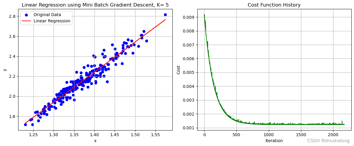
2. 小批量梯度下降法 Mini Batch Gradient Descent(在批量方面进行了改进)
θ 0 : = θ 0 − a 1 N k ∑ i = 1 N k ( f θ ( x ( i ) ) − y ( i ) ) θ 1 : = θ 1 − a 1 N k ∑ i = 1 N k ( f θ ( x ( i ) ) − y ( i ) ) x ( i ) \begin{aligned}\theta_0&:=\theta_0-a\frac1{N_k}\sum_{i=1}^{N_k}(f_\theta\big(x^{(i)}\big)-y^{(i)})\\\theta_1&:=\theta_1-a\frac1{N_k}\sum_{i=1}^{N_k}(f_\theta\big(x^{(i)}\big)-y^{(i)})x^{(i)}\end{aligned} θ0θ1:=θ0−aNk1i=1∑Nk(fθ(x(i))−y(i)):=θ1−aNk1i=1∑Nk(fθ(x(i))−y(i))x(i)
def mini_batch_gradient_descent(x_values, y_values, batch_size=5, alpha=0.05, convergence_threshold=1e-8,max_iterations=10000):"""Perform mini batch gradient descent to learn theta_0 and theta_1.:param x_values: 这是一个list,包含了所有的x值:param y_values: 这是一个list,包含了所有的y值:param batch_size: 这是一个int,表示batch的大小:param alpha: 这是一个float,表示学习率:param convergence_threshold: 这是一个float,表示收敛阈值:param max_iterations: 这是一个int,表示最大迭代次数:return: 这是一个tuple,包含了theta_0, theta_1, cost_history,分别表示最终的theta_0, theta_1和损失函数的变化"""theta_0 = 0 # 初始化theta_0theta_1 = 0 # 初始化theta_1N = len(x_values)cost_history = []for _ in range(max_iterations):# 对数据进行随机打乱combined = list(zip(x_values, y_values)) # 将x_values和y_values打包成一个listrandom.shuffle(combined) # 对打包后的list进行随机打乱x_values[:], y_values[:] = zip(*combined) # 将打乱后的list解包赋值给x_values和y_values# Mini-batch updates# 这里的代码与batch gradient descent的代码类似,只是多了一个batch_size的参数# 对于每一个batch,都会计算一次梯度,并更新theta_0和theta_1for i in range(0, N, batch_size): # i从0开始,每次增加batch_sizex_batch = x_values[i:i + batch_size] # 从i开始,取batch_size个元素y_batch = y_values[i:i + batch_size] # 从i开始,取batch_size个元素sum_theta_0 = 0 # 用来计算theta_0的梯度sum_theta_1 = 0 # 用来计算theta_1的梯度for j in range(len(x_batch)): # 对于每一个batch中的元素error = f_theta(x_batch[j], theta_0, theta_1) - y_batch[j]sum_theta_0 += errorsum_theta_1 += error * x_batch[j]theta_0 -= alpha * (1 / batch_size) * sum_theta_0theta_1 -= alpha * (1 / batch_size) * sum_theta_1cost_history.append(compute_cost(x_values, y_values, theta_0, theta_1))if len(cost_history) > 1 and abs(cost_history[-1] - cost_history[-2]) < convergence_threshold:# 如果损失函数的变化小于收敛阈值,则停止迭代breakreturn theta_0, theta_1, cost_history
# 这一code block用来调用上面的函数# K值的选择需要我们不断尝试与比较,来获取更好的效果
possible_K_values = [1, 3, 4, 5, 6, 7, 10]  # 可能得K值需要自己设定,对于不同的数据集,可能需要不同的K值
best_K = possible_K_values[0]
lowest_cost = float('inf')
theta_0_mini_batch = 0
theta_1_mini_batch = 0
cost_history_mini_batch = []for K in possible_K_values:  # 对于每一个K值theta_0_temp, theta_1_temp, cost_history_temp = mini_batch_gradient_descent(x_values, y_values, K)if cost_history_temp[-1] < lowest_cost:  # 如果损失函数的值更小lowest_cost = cost_history_temp[-1]best_K = Ktheta_0_mini_batch = theta_0_temptheta_1_mini_batch = theta_1_tempcost_history_mini_batch = cost_history_tempbest_K, theta_0_mini_batch, theta_1_mini_batch, lowest_cost
# 这一code block用来画出数据点和拟合直线
plot_data_and_line(x_values, y_values, theta_0_mini_batch, theta_1_mini_batch, cost_history_mini_batch,'Linear Regression using Mini Batch Gradient Descent, K= ' + str(best_K))
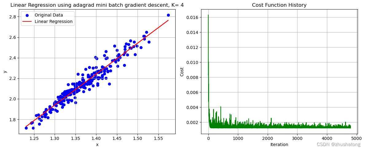
3. 自适应梯度下降法 Adagrad(在学习率方面进行了改进)
θ ( t + 1 ) : = θ ( t ) − a ∑ i = 0 t ( g ( i ) ) 2 g ( t ) \begin{aligned}\theta^{(\mathbf{t+1})}{:}=\theta^{(\mathbf{t})}-\frac{a}{\sqrt{\sum_{i=0}^{t}(g^{(i)})^2}}g^{(t)}\end{aligned} θ(t+1):=θ(t)−∑i=0t(g(i))2ag(t)
其中
g ( t ) = ∂ J ( θ ( t ) ) ∂ θ g^{(t)}=\frac{\partial J(\theta^{(t)})}{\partial\theta} g(t)=∂θ∂J(θ(t))
# 请注意这里的学习率,我将它设定的非常大,得益于adagrad的特性,我们可以使用更大的学习率
# 如果将学习率设定过小,会导致adagrad无法收敛,效果较差
# 所以,我们需要alpha也需要不断尝试与比较,来获取更好的效果
def adagrad_mini_batch_gradient_descent(x_values, y_values, batch_size=5, alpha=3, convergence_threshold=1e-8,max_iterations=10000):"""Perform mini batch gradient descent with adaptive learning rate.:param x_values:  这是一个list,包含了所有的x值:param y_values:  这是一个list,包含了所有的y值:param batch_size:  这是一个int,表示batch的大小:param alpha:   这是一个float,表示学习率:param convergence_threshold:  这是一个float,表示收敛阈值:param max_iterations:  这是一个int,表示最大迭代次数:return:    这是一个tuple,包含了theta_0, theta_1, cost_history,分别表示最终的theta_0, theta_1和损失函数的变化"""theta_0 = 0  # 初始化theta_0theta_1 = 0  # 初始化theta_1N = len(x_values)cost_history = []# 初始化sum_squared_gradients,这是用来计算学习率的sum_squared_gradients_0 = 0.0001  # 较小的值以避免被零除sum_squared_gradients_1 = 0.0001for _ in range(max_iterations):# 对数据进行随机打乱combined = list(zip(x_values, y_values))  # 将x_values和y_values打包成一个listrandom.shuffle(combined)  # 对打包后的list进行随机打乱x_values[:], y_values[:] = zip(*combined)  # 将打乱后的list解包赋值给x_values和y_values# Mini-batch updates# 这里的代码与batch gradient descent的代码类似,只是多了一个batch_size的参数for i in range(0, N, batch_size):x_batch = x_values[i:i + batch_size]y_batch = y_values[i:i + batch_size]sum_theta_0 = 0sum_theta_1 = 0for j in range(len(x_batch)):error = f_theta(x_batch[j], theta_0, theta_1) - y_batch[j]sum_theta_0 += errorsum_theta_1 += error * x_batch[j]# 计算梯度# 计算公式为: theta_j = theta_j - alpha / (sum_squared_gradients_j ** 0.5) * 1/N * sum((f_theta(x_i) - y_i) * x_i)gradient_0 = (1 / batch_size) * sum_theta_0  # 计算theta_0的梯度gradient_1 = (1 / batch_size) * sum_theta_1  # 计算theta_1的梯度sum_squared_gradients_0 += gradient_0 ** 2  # 更新sum_squared_gradients_0sum_squared_gradients_1 += gradient_1 ** 2  # 更新sum_squared_gradients_1adaptive_alpha_0 = alpha / (sum_squared_gradients_0 ** 0.5)  # 计算theta_0的学习率adaptive_alpha_1 = alpha / (sum_squared_gradients_1 ** 0.5)  # 计算theta_1的学习率theta_0 -= adaptive_alpha_0 * gradient_0  # 更新theta_0theta_1 -= adaptive_alpha_1 * gradient_1  # 更新theta_1cost_history.append(compute_cost(x_values, y_values, theta_0, theta_1))if len(cost_history) > 1 and abs(cost_history[-1] - cost_history[-2]) < convergence_threshold:# 如果损失函数的变化小于收敛阈值,则停止迭代breakreturn theta_0, theta_1, cost_history
# 这一code block用来调用上面的函数# K值的选择需要我们不断尝试与比较,来获取更好的效果
possible_K_values = [3, 4, 5, 6, 7, 10]  # 可能得K值需要自己设定,对于不同的数据集,可能需要不同的K值
best_K = possible_K_values[0]
lowest_cost = float('inf')
theta_0_adaptive = 0
theta_1_adaptive = 0
cost_history_adaptive = []for K in possible_K_values:  # 对于每一个K值theta_0_temp, theta_1_temp, cost_history_temp = adagrad_mini_batch_gradient_descent(x_values, y_values, K)if cost_history_temp[-1] < lowest_cost:lowest_cost = cost_history_temp[-1]best_K = Ktheta_0_adaptive = theta_0_temptheta_1_adaptive = theta_1_tempcost_history_adaptive = cost_history_tempbest_K, theta_0_adaptive, theta_1_adaptive, cost_history_adaptive[-1]
# 这一code block用来画出数据点和拟合直线
plot_data_and_line(x_values, y_values, theta_0_adaptive, theta_1_adaptive, cost_history_adaptive,'Linear Regression using adagrad mini batch gradient descent, K= ' + str(best_K))
4. 多变量线性回归 Multivariate Linear Regression(在特征方面进行了改进,拓展到多个特征)
f θ ( x ) = θ 0 + θ 1 x 1 + θ 2 x 2 + ⋯ + θ n x n f_\theta(x)=\theta_0+\theta_1x_1+\theta_2x_2+\cdots+\theta_nx_n fθ(x)=θ0+θ1x1+θ2x2+⋯+θnxn
J ( θ 0 , θ 1 , . . . θ n ) = 1 2 N ∑ i = 1 N ( f θ ( x ( i ) ) − y ( i ) ) 2 J(\theta_0,\theta_1,...\theta_n)=\frac1{2N}\sum_{i=1}^N(f_\theta(x^{(i)})-y^{(i)})^2 J(θ0,θ1,...θn)=2N1i=1∑N(fθ(x(i))−y(i))2
def multivariate_gradient_descent(X, y, batch_size=5, alpha=3, convergence_threshold=1e-8, max_iterations=10000):"""Perform mini batch gradient descent with adaptive learning rate for multivariate linear regression.:param X: 这是一个矩阵,包含了所有的x值:param y: 这是一个list,包含了所有的y值:param batch_size: 这是一个int,表示batch的大小:param alpha: 这是一个float,表示学习率:param convergence_threshold: 这是一个float,表示收敛阈值:param max_iterations: 这是一个int,表示最大迭代次数:return: 这是一个tuple,包含了theta, cost_history,分别表示最终的theta和损失函数的变化,theta是一个list"""m, n = X.shape # m是样本数量,n是特征数量theta = np.zeros(n + 1) # n+1 thetas 包含 theta_0X = np.hstack((np.ones((m, 1)), X)) # 在X前面加一列1,用来计算theta_0cost_history = []sum_squared_gradients = np.zeros(n + 1) + 0.0001 # 较小的值以避免被零除for _ in range(max_iterations):# 对数据进行随机打乱indices = np.arange(m) # 生成一个0到m-1的listnp.random.shuffle(indices) # 对list进行随机打乱X = X[indices] # 用打乱后的list对X进行重新排序y = y[indices] # 用打乱后的list对y进行重新排序# Mini-batch updatesfor i in range(0, m, batch_size): # i从0开始,每次增加batch_sizeX_batch = X[i:i + batch_size] # 从i开始,取batch_size个元素y_batch = y[i:i + batch_size] # 从i开始,取batch_size个元素# 梯度计算公式为: theta_j = theta_j - alpha / (sum_squared_gradients_j ** 0.5) * 1/N * sum((f_theta(x_i) - y_i) * x_i) gradient = (1 / batch_size) * X_batch.T.dot(X_batch.dot(theta) - y_batch) # 计算梯度sum_squared_gradients += gradient ** 2 # 更新sum_squared_gradientsadaptive_alpha = alpha / np.sqrt(sum_squared_gradients) # 计算学习率theta -= adaptive_alpha * gradient # 更新thetacost = (1 / (2 * m)) * np.sum((X.dot(theta) - y) ** 2) # 计算损失函数的值cost_history.append(cost)if len(cost_history) > 1 and abs(cost_history[-1] - cost_history[-2]) < convergence_threshold:# 如果损失函数的变化小于收敛阈值,则停止迭代breakreturn theta, cost_history
# 这一code block用来调用上面的函数
# 请注意,这里的数据集是多变量线性回归的数据集
X_matrix = data[['x']].values
y_vector = data['y'].values
# best_K 已经在上面的代码中被赋值
theta_multivariate, cost_history_multivariate = multivariate_gradient_descent(X_matrix, y_vector, best_K)theta_multivariate, cost_history_multivariate[-1]
5. L1正则化 L1 Regularization(在正则化方面进行了改进)
线性回归——lasso回归和岭回归(ridge regression) - wuliytTaotao - 博客园 (cnblogs.com)
def lasso_gradient_descent(X, y, batch_size=5, lambda_=0.1, alpha=3, convergence_threshold=1e-8, max_iterations=10000):"""Perform mini batch gradient descent with adaptive learning rate and L1 regularization for multivariate linear regression."""m, n = X.shape # m是样本数量,n是特征数量theta = np.zeros(n + 1) # n+1 thetas 包含 theta_0X = np.hstack((np.ones((m, 1)), X)) # 在X前面加一列1,用来计算theta_0cost_history = []sum_squared_gradients = np.zeros(n + 1) + 0.0001 # 较小的值以避免被零除for _ in range(max_iterations):# 对数据进行随机打乱indices = np.arange(m) # 生成一个0到m-1的listnp.random.shuffle(indices) # 对list进行随机打乱X = X[indices] # 用打乱后的list对X进行重新排序y = y[indices] # 用打乱后的list对y进行重新排序# Mini-batch updatesfor i in range(0, m, batch_size): # i从0开始,每次增加batch_sizeX_batch = X[i:i + batch_size] # 从i开始,取batch_size个元素y_batch = y[i:i + batch_size] # 从i开始,取batch_size个元素# Compute gradient (including L1 penalty for j > 0)gradient = (1 / batch_size) * X_batch.T.dot(X_batch.dot(theta) - y_batch) # 计算梯度gradient[1:] += lambda_ * np.sign(theta[1:]) # 对除theta_0外的所有theta添加L1正则化sum_squared_gradients += gradient ** 2 # 更新sum_squared_gradientsadaptive_alpha = alpha / np.sqrt(sum_squared_gradients) # 计算学习率theta -= adaptive_alpha * gradient # 更新theta# Compute cost (including L1 penalty for j > 0)cost = (1 / (2 * m)) * np.sum((X.dot(theta) - y) ** 2) + lambda_ * np.sum(np.abs(theta[1:]))cost_history.append(cost)if len(cost_history) > 1 and abs(cost_history[-1] - cost_history[-2]) < convergence_threshold:# 如果损失函数的变化小于收敛阈值,则停止迭代breakreturn theta, cost_history
如何选择lambda?
def determine_best_lambda(X, y, lambdas, num_folds=5, **kwargs):"""Determine the best lambda using K-fold cross validation."""from sklearn.model_selection import KFold # 此处使用sklearn中的KFold函数,用来进行交叉验证,与线性回归无关kf = KFold(n_splits=num_folds, shuffle=True, random_state=42) # 生成交叉验证的数据,42是随机种子average_errors = [] # 用来保存每一个lambda的平均误差for lambda_ in lambdas: # 对于每一个lambdafold_errors = [] # 用来保存每一折的误差for train_index, val_index in kf.split(X):X_train, X_val = X[train_index], X[val_index] # 生成训练集和验证集y_train, y_val = y[train_index], y[val_index] # 生成训练集和验证集theta, _ = lasso_gradient_descent(X_train, y_train, lambda_=lambda_, **kwargs) # 训练模型# Compute validation errory_pred = np.hstack((np.ones((X_val.shape[0], 1)), X_val)).dot(theta) # 计算预测值error = (1 / (2 * X_val.shape[0])) * np.sum((y_pred - y_val) ** 2) # 计算误差fold_errors.append(error)average_errors.append(np.mean(fold_errors))best_lambda = lambdas[np.argmin(average_errors)] # 选择平均误差最小的lambdareturn best_lambda, average_errors
# Lambda values to test
lambdas = [0, 0.001, 0.01, 0.1, 1, 10]best_lambda, average_errors = determine_best_lambda(X_matrix, y_vector, lambdas)
best_lambda, average_errors
# Apply the multivariate gradient descent (using the single feature we have for this dataset)
X_matrix = data[['x']].values
y_vector = data['y'].values
theta_lasso, cost_history_lasso = lasso_gradient_descent(X_matrix, y_vector, best_K, best_lambda)theta_lasso, cost_history_lasso[-1]# 选择平均误差最小的lambdareturn best_lambda, average_errors
相关文章:
【机器学习】从底层手写实现线性回归
【机器学习】Building-Linear-Regression-from-Scratch 线性回归 Linear Regression0. 数据的导入与相关预处理0.工具函数1. 批量梯度下降法 Batch Gradient Descent2. 小批量梯度下降法 Mini Batch Gradient Descent(在批量方面进行了改进)3. 自适应梯度…...

判断数组中对象的某个值是否有相同的并去重
如果你想判断数组中对象的某个值是否有相同的,并进行去重,你可以使用 JavaScript 中的一些数组方法和 Set 对象。以下是一个示例: // 原始数组包含对象 const array [{ id: 1, name: John },{ id: 2, name: Jane },{ id: 3, name: Doe },{ …...

Shell脚本 变量 语句 表达式
常见的解释器 #!/bin/sh #不推荐(了解) #!/bin/bash #!/usr/bin/python #!/bin/awk#!后跟的字符表示要启动的程序,该程序读取该文件执行。 #! 是一个约定的标记,它告诉系统这个脚本需要什么解释器来执行shell 函数 myShellName () {command1 }函数调用…...
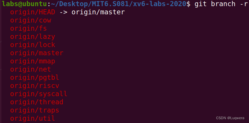
MIT6.S081-实验准备
实验全程在Vmware虚拟机 (镜像:Ubuntu-20.04-beta-desktop-amd64) 中进行 一、版本控制 1.1 将mit的实验代码克隆到本地 git clone git://g.csail.mit.edu/xv6-labs-2020 1.2 修改本地git配置文件 创建github仓库,记录仓库地址 我的仓库地址就是htt…...

工具在手,创作无忧:一键下载安装Auto CAD工具,让艺术创作更加轻松愉悦!
不要再浪费时间在网上寻找Auto CAD的安装包了!因为你所需的一切都可以在这里找到!作为全球领先的设计和绘图软件,Auto CAD为艺术家、设计师和工程师们提供了无限的创作潜力。不论是建筑设计、工业设计还是室内装饰,Auto CAD都能助…...

第25节: Vue3 带组件
在UniApp中使用Vue3框架时,你可以使用组件来封装可复用的代码块,并在需要的地方进行渲染。下面是一个示例,演示了如何在UniApp中使用Vue3框架使用带组件: <template> <view> <button click"toggleActive&q…...

ubuntu apache2配置反向代理
1.Ubuntu安装apache sudo apt-get update sudo apt-get install apache2 2.apache2反向代理配置 sudo vim /etc/apache2/sites-available/000-default.conf 添加内容如下: <VirtualHost *:80># The ServerName directive sets the request scheme, host…...

【数据挖掘 | 关联规则】FP-grow算法详解(附详细代码、案例实战、学习资源)
! 🤵♂️ 个人主页: AI_magician 📡主页地址: 作者简介:CSDN内容合伙人,全栈领域优质创作者。 👨💻景愿:旨在于能和更多的热爱计算机的伙伴一起成长!!&a…...
 11)
力扣题目学习笔记(OC + Swift) 11
11.盛最多水的容器 给定一个长度为 n 的整数数组 height 。有 n 条垂线,第 i 条线的两个端点是 (i, 0) 和 (i, height[i]) 。 找出其中的两条线,使得它们与 x 轴共同构成的容器可以容纳最多的水。 返回容器可以储存的最大水量。 说明:你不能倾…...
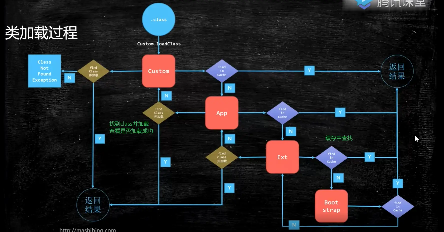
JVM基础入门
JVM 基础入门 JVM 基础 聊一聊 Java 从编码到执行到底是一个怎么样的过程? 假设我们有一个文件 x.Java,你执行 javac,它就会变成 x.class。 这个 class 怎么执行的? 当我们调用 Java 命令的时候,class 会被 load 到…...

前端真的死了吗
随着人工智能和低代码的崛起,“前端已死”的声音逐渐兴起。前端已死?尊嘟假嘟?快来发表你的看法吧! 以下方向仅供参考。 一、为什么会出现“前端已死”的言论 前端已死这个言论 是出自于2022年开始 ,2022年下半年疫情…...

前后端分离开发
前期 前后端混合开发 后期 前后端分离开发...
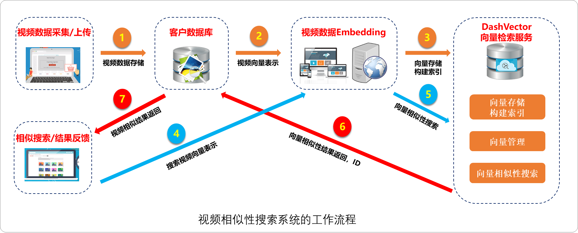
向量数据库——AI时代的基座
向量数据库——AI时代的基座 1.前言 向量数据库在构建基于大语言模型的行业智能应用中扮演着重要角色。大模型虽然能回答一般性问题,但在垂直领域服务中,其知识深度、准确度和时效性有限。为了解决这一问题,企业可以利用向量数据库结合大模…...
【️什么是分布式系统的一致性 ?】
😊引言 🎖️本篇博文约8000字,阅读大约30分钟,亲爱的读者,如果本博文对您有帮助,欢迎点赞关注!😊😊😊 🖥️什么是分布式系统的一致性 ?…...
鸿蒙ArkTS Web组件加载空白的问题原因及解决方案
问题症状 初学鸿蒙开发,按照官方文档Web组件文档《使用Web组件加载页面》示例中的代码照抄运行后显示空白,纠结之余多方搜索后扔无解决方法。 运行代码 import web_webview from ohos.web.webviewEntry Component struct Index {controller: web_webv…...
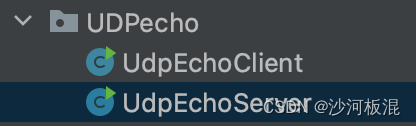
【Java】网络编程-UDP回响服务器客户端简单代码编写
这一篇文章我们将讲述网络编程中UDP服务器客户端的编程代码 1、前置知识 UDP协议全称是用户数据报协议,在网络中它与TCP协议一样用于处理数据包,是一种无连接的协议。 UDP的特点有:无连接、尽最大努力交付、面向报文、没有拥塞控制 本文讲…...

【设计模式】之工厂模式
工厂模式 1.介绍 工厂模式(创建型模式),是我们最常用的实例化对象模式,是用工厂方法代替new操作的一种模式;在工厂模式中,我们在创建对象时不会对客户端暴露创建逻辑,并且是通过使用一个共同的…...

70.爬楼梯
题目描述 假设你正在爬楼梯。需要 n 阶你才能到达楼顶。 每次你可以爬 1 或 2 个台阶。你有多少种不同的方法可以爬到楼顶呢? 注意: 给定 n 是一个正整数。 示例 1: 输入: 2 输出: 2 解释: 有两种方法可以爬到楼顶…...
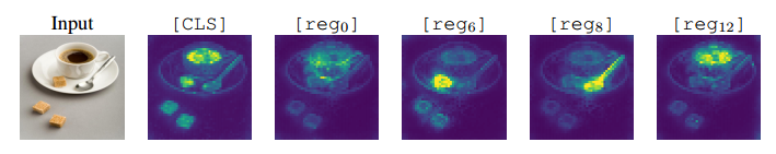
【论文解读】ICLR 2024高分作:ViT需要寄存器
来源:投稿 作者:橡皮 编辑:学姐 论文链接:https://arxiv.org/abs/2309.16588 摘要: Transformer最近已成为学习视觉表示的强大工具。在本文中,我们识别并表征监督和自监督 ViT 网络的特征图中的伪影。这些…...
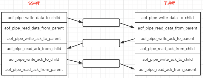
【Redis】AOF 基础
因为 Redis AOF 的实现有些绕, 就分成 2 篇进行分析, 本篇主要是介绍一下 AOF 的一些特性和依赖的其他函数的逻辑,为下一篇 (Redis AOF 源码) 源码分析做一些铺垫。 AOF 全称: Append Only File, 是 Redis 提供了一种数据保存模式, Redis 默认不开启。 AOF 采用日志的形式来记…...

一U多系统终极方案:用Ventoy管理ISO镜像+VMware验证的完整工作流
一U多系统终极方案:用Ventoy管理ISO镜像与VMware验证的完整工作流 在数字工具日益复杂的今天,系统管理员和技术爱好者常面临一个经典难题:如何高效管理多个操作系统镜像并确保其启动兼容性。传统方法需要反复格式化U盘或携带多个启动设备&am…...

JavaScript DXF文件生成:在浏览器中创建CAD图纸的终极方案
JavaScript DXF文件生成:在浏览器中创建CAD图纸的终极方案 【免费下载链接】js-dxf JavaScript DXF writer 项目地址: https://gitcode.com/gh_mirrors/js/js-dxf 你是否需要在Web应用中集成工程图纸生成功能?JavaScript DXF文件生成库为你提供了…...

CoPaw赋能智慧医疗:辅助电子病历分析与报告生成
CoPaw赋能智慧医疗:辅助电子病历分析与报告生成 1. 医疗文书处理的痛点与机遇 早上8点,张医生刚走进诊室,电脑上已经堆积了30多份待处理的电子病历。每份病历都包含患者主诉、检查结果、既往病史等非结构化文本,需要人工提取关键…...

昇腾算子开发知识地图
作者:昇腾实战派 背景 本博客旨在对社区发表的昇腾算子相关博客进行整理归类,方便用户导航使用;以下文章所用的机器均为昇腾相关设备。 Ascend C 基础理论 Ascend C基础 Ascend C算子开发详解:从原理到实战的深度剖析 深入A…...

窗口大小强制调整工具终极指南:如何轻松掌控任意应用程序窗口尺寸
窗口大小强制调整工具终极指南:如何轻松掌控任意应用程序窗口尺寸 【免费下载链接】WindowResizer 一个可以强制调整应用程序窗口大小的工具 项目地址: https://gitcode.com/gh_mirrors/wi/WindowResizer 还在为那些顽固的应用程序窗口而烦恼吗?某…...

Windows驱动级输入模拟终极指南:Interceptor技术深度解析与应用实战
Windows驱动级输入模拟终极指南:Interceptor技术深度解析与应用实战 【免费下载链接】Interceptor C# wrapper for a Windows keyboard driver. Can simulate keystrokes and mouse clicks in protected areas like the Windows logon screen (and yes, even in gam…...

科研人投稿破局:Paperxie AI 期刊写作,把「拒稿重写」变成「一次过审」
paperxie-免费查重复率aigc检测/开题报告/毕业论文/智能排版/文献综述/期刊论文https://www.paperxie.cn/ai/journalArticleshttps://www.paperxie.cn/ai/journalArticles 在学术圈,「写期刊论文」从来都不是敲字那么简单 —— 要贴合期刊收稿方向、要挖创新点、要卡…...

Agent 帮不了你,不是因为它不够聪明
上一篇我们分析了 CLI vs MCP 的争论本质上是在讨论"管道",而真正缺的是"水龙头"。这篇继续往下挖:就算水龙头开了,你也大概率接不上。Agent 在现实中寸步难行的原因,比大多数人想的更结构化。 一个常见的许诺…...

Apifox 实战:从实体类到请求参数的自动化转换技巧
1. 为什么需要实体类到请求参数的自动化转换 每次对接新接口时最头疼的事情是什么?对我来说就是手动编写那一大堆请求参数。上周接手一个用户管理模块,光是用户信息更新接口就有23个字段,如果每个字段都要手动填写参数名、类型、说明…...

OpenClaw 2026年阿里云8分钟本地云端集成零基础部署及使用教程
OpenClaw 2026年阿里云8分钟本地云端集成零基础部署及使用教程。本文面向零基础用户,完整说明在轻量服务器与本地Windows11、macOS、Linux系统中部署OpenClaw(Clawdbot)的流程,包含环境配置、服务启动、Skills集成、阿里云百炼API…...