Kaggle竞赛系列_SpaceshipTitanic金牌方案分析_数据分析
文章目录
- 【文章系列】
- 【前言】
- 【比赛简介】
- 【正文】
- (一)数据获取
- (二)数据分析
- 1. 缺失值
- 2. 重复值
- 3. 属性类型分析
- 4. 类别分析
- 5. 分析目标数值占比
- (三)属性分析
- 1. 对年龄Age分析
- (1)直方图分析
- (2)创建新属性
- 2. 对支出属性进行分析
- (1)直方图分析
- (2)创建新属性
- 3. 对离散属性进行分析
- (1)直方图分析
- 4. 对定性属性进行分析
- (1)属性分析
- (2)根据PassengerId划分group
- (3)对Cabin属性进一步划分
- (4)根据Name的姓氏划分出家庭组
- (四)归纳总结
- (五)写在最后
【文章系列】
第一章 初探Kaggle竞赛————Kaggle竞赛系列_Titanic比赛
第二章 知识补充_随机森林————数学建模系列_随机森林
第三章 知识补充_LightGBM————集成学习之Boosting方法系列_LightGBM
第四章 再战Kaggle竞赛————Kaggle竞赛系列_SpaceshipTitanic比赛
第五章 重温回顾_学习金牌方法_数据分析————Kaggle竞赛系列_SpaceshipTitanic金牌方案分析_数据分析
第六章 重温回顾_学习金牌方法_数据处理————Kaggle竞赛系列_SpaceshipTitanic金牌方案分析_数据处理
【前言】
Spaceship Titanic比赛,类似Titanic比赛,只是增加了更多的属性以及更大的数据量,仍是一个二分类问题。
今天要分析的是一篇大神的解决方案,看完后觉得干货满满,由衷地敬佩他们对数据分析的细致程度,对比之下只觉得之前自己的分析仅仅是表面功夫,单纯靠着模型的强大能力去完成任务。看来以后还是得不断地向各位前辈大佬学习,完善自己的解决方案!!!
项目代码 : 🚀 Spaceship Titanic: A complete guide 🏆 | Kaggle
我的解决方案:Kaggle竞赛系列_SpaceshipTitanic比赛
【比赛简介】
Spaceship Titanic比赛是一个在Kaggle上举办的机器学习挑战,参赛者的任务是预测Spaceship Titanic在与时空异常碰撞时,哪些乘客被传送到了另一个维度。这个比赛提供了从飞船损坏的计算机系统中恢复的一组个人记录,参赛者需要使用这些数据来进行预测。
【正文】
(一)数据获取
参考之前的Titanic比赛的数据获取操作 Kaggle_Titanic比赛
(二)数据分析
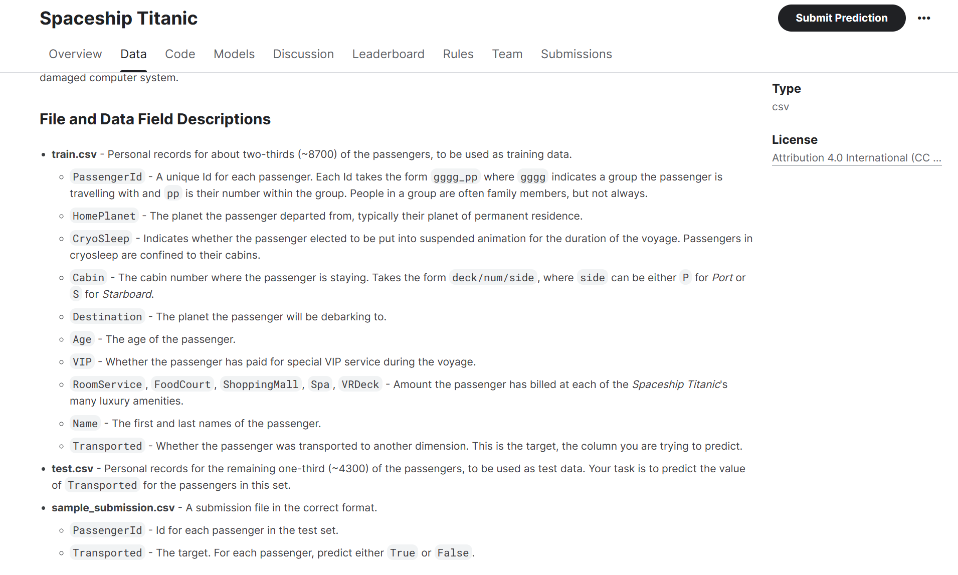
train.csv- 用于训练数据的大约三分之二(约8700名)乘客的个人记录。PassengerId- 每位乘客的唯一标识。每个标识的格式为gggg_pp,其中gggg表示乘客所在的团体,pp是他们在团体中的编号。一个团体中的人通常是家庭成员,但并不总是如此。HomePlanet- 乘客出发的星球,通常是他们的永久居住星球。CryoSleep- 表示乘客是否选择在航程期间被置于悬浮动状态。处于冷冻睡眠状态的乘客被限制在他们的舱房内。Cabin- 乘客所住的舱房号码。格式为deck/num/side,其中side可以是P(港口)或S(舷侧)。Destination- 乘客将要下船的星球。Age- 乘客的年龄。VIP- 乘客是否支付额外费用获得特殊的VIP服务。RoomService,FoodCourt,ShoppingMall,Spa,VRDeck- 乘客在太空巨轮泰坦尼克号的许多豪华设施上的费用金额。Name- 乘客的名字和姓氏。Transported- 乘客是否被传送到另一个维度。这是目标,也就是您要预测的列。test.csv- 剩余三分之一(约4300名)乘客的个人记录,用作测试数据。您的任务是预测这一集合中乘客的Transported值。sample_submission.csv- 一个以正确格式的提交文件。PassengerId- 测试集中每位乘客的标识。Transported- 目标。对于每位乘客,预测True或False。
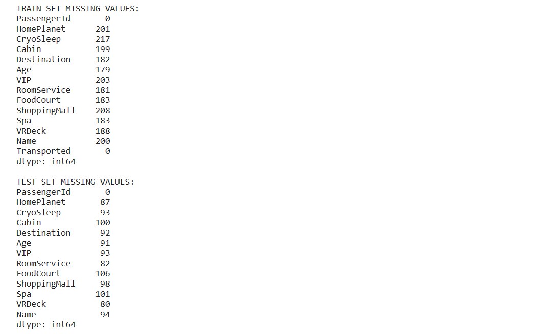
1. 缺失值
print('TRAIN SET MISSING VALUES:')
print(train.isna().sum())
print('')
print('TEST SET MISSING VALUES:')
print(test.isna().sum())
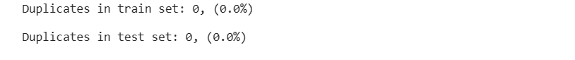
2. 重复值
print(f'Duplicates in train set: {train.duplicated().sum()}, ({np.round(100*train.duplicated().sum()/len(train),1)}%)')
print('')
print(f'Duplicates in test set: {test.duplicated().sum()}, ({np.round(100*test.duplicated().sum()/len(test),1)}%)')
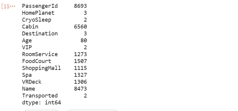
3. 属性类型分析
train.nunique()
4. 类别分析
train.dtypes
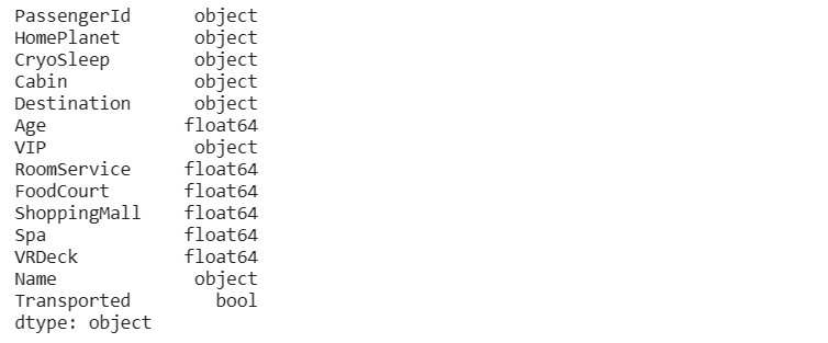
一般而言,连续型属性被存储为float和double类型,离散型属性被存储为object和int类型。
- 6个连续性属性(
RoomService,FoodCourt,ShoppingMall,Spa,VRDeck,Age) - 4个离散属性(
HomePlanet,CryoSleep,Destination,VIP) - 剩余3个描述性/定性属性(
PassengerId,Name,Cabin)
5. 分析目标数值占比
# 特征尺寸
plt.figure(figsize=(6,6))# 饼状图
train['Transported'].value_counts().plot.pie(explode=[0.1,0.1], autopct='%1.1f%%', shadow=True, textprops={'fontsize':16}).set_title("Target distribution")
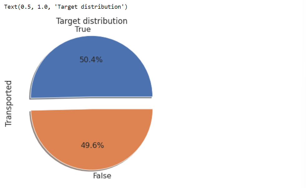
分布平衡,因此不需要采用过采样、欠采样方法。
(三)属性分析
1. 对年龄Age分析
(1)直方图分析
直方图关键参数:hue=Target属性
# 特征尺寸
plt.figure(figsize=(10,4))# 直方图
sns.histplot(data=train, x='Age', hue='Transported', binwidth=1, kde=True)plt.title('Age distribution')
plt.xlabel('Age (years)')
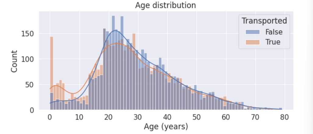
注意到:
- 0-18岁的青少年更容易被转移。
- 18-25岁的人被转移的可能性比不被转移的可能性要小。
- 25岁以上的人被转移的可能性和没有被转移的可能性差不多。
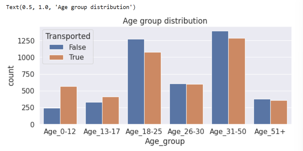
(2)创建新属性
根据直方图False与True的高度关系,对年龄划分为多层,并依次建立一个新特征。
# 新特征-训练集
train['Age_group']=np.nan
train.loc[train['Age']<=12,'Age_group']='Age_0-12'
train.loc[(train['Age']>12) & (train['Age']<18),'Age_group']='Age_13-17'
train.loc[(train['Age']>=18) & (train['Age']<=25),'Age_group']='Age_18-25'
train.loc[(train['Age']>25) & (train['Age']<=30),'Age_group']='Age_26-30'
train.loc[(train['Age']>30) & (train['Age']<=50),'Age_group']='Age_31-50'
train.loc[train['Age']>50,'Age_group']='Age_51+'# 新特征-测试集
test['Age_group']=np.nan
test.loc[test['Age']<=12,'Age_group']='Age_0-12'
test.loc[(test['Age']>12) & (test['Age']<18),'Age_group']='Age_13-17'
test.loc[(test['Age']>=18) & (test['Age']<=25),'Age_group']='Age_18-25'
test.loc[(test['Age']>25) & (test['Age']<=30),'Age_group']='Age_26-30'
test.loc[(test['Age']>30) & (test['Age']<=50),'Age_group']='Age_31-50'
test.loc[test['Age']>50,'Age_group']='Age_51+'# 新特征的分布图
plt.figure(figsize=(10,4))
g=sns.countplot(data=train, x='Age_group', hue='Transported', order=['Age_0-12','Age_13-17','Age_18-25','Age_26-30','Age_31-50','Age_51+'])
plt.title('Age group distribution')
2. 对支出属性进行分析
(1)直方图分析
# 支出特征
exp_feats=['RoomService', 'FoodCourt', 'ShoppingMall', 'Spa', 'VRDeck']# 绘图
fig=plt.figure(figsize=(10,20))
for i, var_name in enumerate(exp_feats):# 左图ax=fig.add_subplot(5,2,2*i+1)sns.histplot(data=train, x=var_name, axes=ax, bins=30, kde=False, hue='Transported')ax.set_title(var_name)# 右图(核密度估计)ax=fig.add_subplot(5,2,2*i+2)sns.histplot(data=train, x=var_name, axes=ax, bins=30, kde=True, hue='Transported')plt.ylim([0,100])ax.set_title(var_name)
fig.tight_layout()  # 改善外观
plt.show()
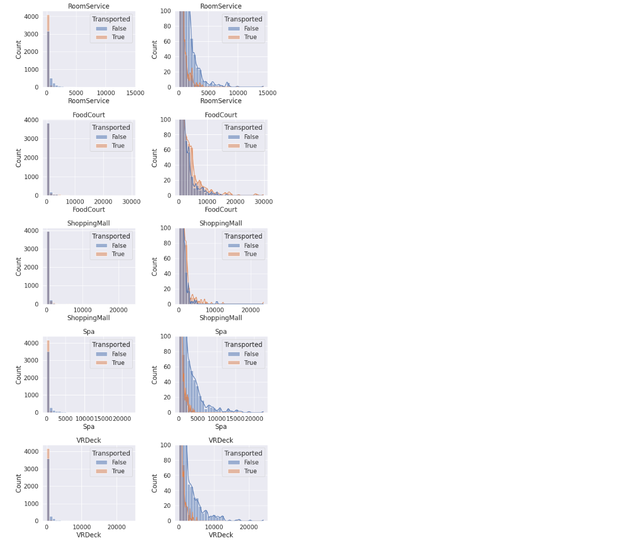
注意到:
- 大多数人都没有花钱,因此可以创建一个二元属性对是否有支出进行划分。
- 有少数的异常值。
- 被运输的人往往花费更少。
- RoomService、Spa和VRDeck与FoodCourt和ShoppingMall有着不同的分布
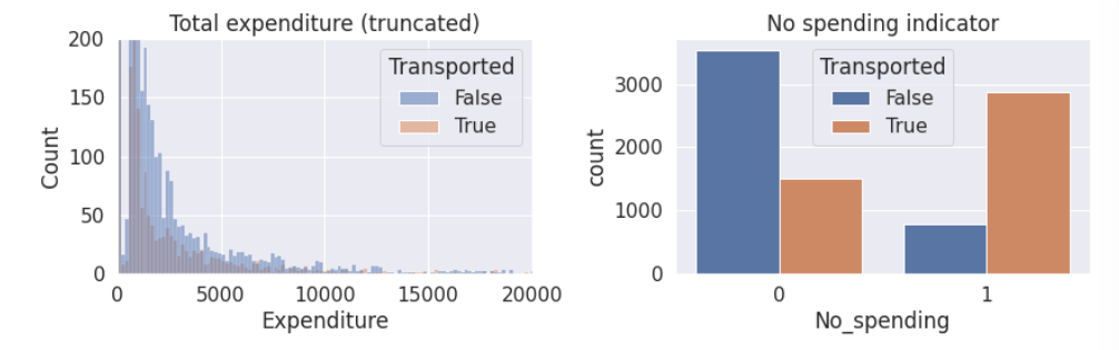
(2)创建新属性
创建一个新属性记录5个支出属性的总开支。再创建一个二元属性对是否有支出进行划分。
# 新特征-训练集
train['Expenditure']=train[exp_feats].sum(axis=1)
train['No_spending']=(train['Expenditure']==0).astype(int)# 新特征-测试集
test['Expenditure']=test[exp_feats].sum(axis=1)
test['No_spending']=(test['Expenditure']==0).astype(int)# 新特征的分布图
fig=plt.figure(figsize=(12,4))
plt.subplot(1,2,1)
sns.histplot(data=train, x='Expenditure', hue='Transported', bins=200)
plt.title('Total expenditure (truncated)')
plt.ylim([0,200])
plt.xlim([0,20000])plt.subplot(1,2,2)
sns.countplot(data=train, x='No_spending', hue='Transported')
plt.title('No spending indicator')
fig.tight_layout()
3. 对离散属性进行分析
(1)直方图分析
离散属性——>countplot
# 离散特征
cat_feats=['HomePlanet', 'CryoSleep', 'Destination', 'VIP']# 绘图
fig=plt.figure(figsize=(10,16))
for i, var_name in enumerate(cat_feats):ax=fig.add_subplot(4,1,i+1)sns.countplot(data=train, x=var_name, axes=ax, hue='Transported')ax.set_title(var_name)
fig.tight_layout()  # 改善外观
plt.show()
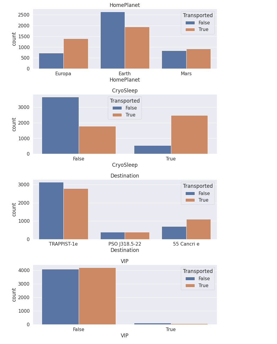
注意到:
- VIP似乎不是一个有用的功能,对目标分割差不多相等。相比之下,CryoSleep似乎是一个非常有用的功能。因此我们可以考虑去掉VIP列以防止过拟合。
4. 对定性属性进行分析
(1)属性分析
# 定性特征
qual_feats=['PassengerId', 'Cabin' ,'Name']# 预览定性特征
train[qual_feats].head()
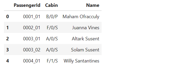
注意到:
- Passengerld采用gggg_pp的形式,其中gggg表示乘客所在的旅行团,pp表示他们在旅行团中的编号。
- Cabin的形式为deck/num/side,其中side可以是P代表左舷,也可以是S代表右舷。
因此我们可以从Passengerld特征中提取群组和群组大小。从Cabin特征中提取甲板、数量和侧面。从Name特征中提取姓氏来识别家庭。
(2)根据PassengerId划分group
# 新特征-分组
train['Group'] = train['PassengerId'].apply(lambda x: x.split('_')[0]).astype(int)
test['Group'] = test['PassengerId'].apply(lambda x: x.split('_')[0]).astype(int)# 绘图
plt.figure(figsize=(20,4))
plt.subplot(1,2,1)
sns.histplot(data=train, x='Group', hue='Transported', binwidth=1)
plt.title('Group')
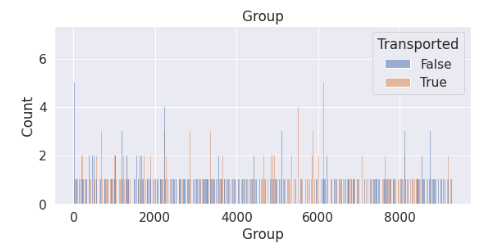
发现分组过多,不好进行独热编码,因此新建一个属性根据分组的人数记录每个分组的数量。
# 新特征-分组大小
train['Group_size']=train['Group'].map(lambda x: pd.concat([train['Group'], test['Group']]).value_counts()[x])
test['Group_size']=test['Group'].map(lambda x: pd.concat([train['Group'], test['Group']]).value_counts()[x])plt.subplot(1,2,2)
sns.countplot(data=train, x='Group_size', hue='Transported')
plt.title('Group size')
fig.tight_layout()
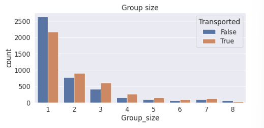
发现除了1人组更不容易被传输,其他人数的分组基本上都是更容易被传输,因此可以将其他人数的分组划分在一起。为此我们可以再新建一个属性来判断该数据是否是1人组(是否独自出行)。
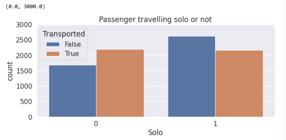
# 新特征
train['Solo']=(train['Group_size']==1).astype(int)
test['Solo']=(test['Group_size']==1).astype(int)# 新特质分布图
plt.figure(figsize=(10,4))
sns.countplot(data=train, x='Solo', hue='Transported')
plt.title('Passenger travelling solo or not')
plt.ylim([0,3000])
(3)对Cabin属性进一步划分
# 现在用离群值替换NaN(这样我们就可以拆分特征)
train['Cabin'].fillna('Z/9999/Z', inplace=True)
test['Cabin'].fillna('Z/9999/Z', inplace=True)#  新特征-训练集
train['Cabin_deck'] = train['Cabin'].apply(lambda x: x.split('/')[0])
train['Cabin_number'] = train['Cabin'].apply(lambda x: x.split('/')[1]).astype(int)
train['Cabin_side'] = train['Cabin'].apply(lambda x: x.split('/')[2])#  新特征-测试集
test['Cabin_deck'] = test['Cabin'].apply(lambda x: x.split('/')[0])
test['Cabin_number'] = test['Cabin'].apply(lambda x: x.split('/')[1]).astype(int)
test['Cabin_side'] = test['Cabin'].apply(lambda x: x.split('/')[2])# 把Nan的放回去(我们稍后会填充这些)
train.loc[train['Cabin_deck']=='Z', 'Cabin_deck']=np.nan
train.loc[train['Cabin_number']==9999, 'Cabin_number']=np.nan
train.loc[train['Cabin_side']=='Z', 'Cabin_side']=np.nan
test.loc[test['Cabin_deck']=='Z', 'Cabin_deck']=np.nan
test.loc[test['Cabin_number']==9999, 'Cabin_number']=np.nan
test.loc[test['Cabin_side']=='Z', 'Cabin_side']=np.nan# 丢弃Cabin属性(我们不再需要它了)
train.drop('Cabin', axis=1, inplace=True)
test.drop('Cabin', axis=1, inplace=True)# 新特征的分布图
fig=plt.figure(figsize=(10,12))
plt.subplot(3,1,1)
sns.countplot(data=train, x='Cabin_deck', hue='Transported', order=['A','B','C','D','E','F','G','T'])
plt.title('Cabin deck')plt.subplot(3,1,2)
sns.histplot(data=train, x='Cabin_number', hue='Transported',binwidth=20)
plt.vlines(300, ymin=0, ymax=200, color='black')
plt.vlines(600, ymin=0, ymax=200, color='black')
plt.vlines(900, ymin=0, ymax=200, color='black')
plt.vlines(1200, ymin=0, ymax=200, color='black')
plt.vlines(1500, ymin=0, ymax=200, color='black')
plt.vlines(1800, ymin=0, ymax=200, color='black')
plt.title('Cabin number')
plt.xlim([0,2000])plt.subplot(3,1,3)
sns.countplot(data=train, x='Cabin_side', hue='Transported')
plt.title('Cabin side')
fig.tight_layout()
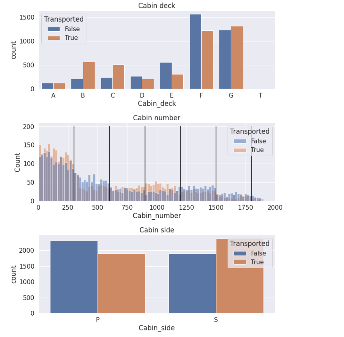
注意到Cabin_number被按照300的数量进行划分,每个划分的False与True的高度都不一样。这意味着我们可以压缩这个特征被压缩成一个分类特征,其他注意事项:客舱甲板的“T”似乎是一个异常值(只有5个样本)。
# 新特征-训练集
train['Cabin_region1']=(train['Cabin_number']<300).astype(int) # 独热编码
train['Cabin_region2']=((train['Cabin_number']>=300) & (train['Cabin_number']<600)).astype(int)
train['Cabin_region3']=((train['Cabin_number']>=600) & (train['Cabin_number']<900)).astype(int)
train['Cabin_region4']=((train['Cabin_number']>=900) & (train['Cabin_number']<1200)).astype(int)
train['Cabin_region5']=((train['Cabin_number']>=1200) & (train['Cabin_number']<1500)).astype(int)
train['Cabin_region6']=((train['Cabin_number']>=1500) & (train['Cabin_number']<1800)).astype(int)
train['Cabin_region7']=(train['Cabin_number']>=1800).astype(int)# 新特征-测试集
test['Cabin_region1']=(test['Cabin_number']<300).astype(int) # 独热编码
test['Cabin_region2']=((test['Cabin_number']>=300) & (test['Cabin_number']<600)).astype(int)
test['Cabin_region3']=((test['Cabin_number']>=600) & (test['Cabin_number']<900)).astype(int)
test['Cabin_region4']=((test['Cabin_number']>=900) & (test['Cabin_number']<1200)).astype(int)
test['Cabin_region5']=((test['Cabin_number']>=1200) & (test['Cabin_number']<1500)).astype(int)
test['Cabin_region6']=((test['Cabin_number']>=1500) & (test['Cabin_number']<1800)).astype(int)
test['Cabin_region7']=(test['Cabin_number']>=1800).astype(int)# 新特征的分布图
plt.figure(figsize=(10,4))
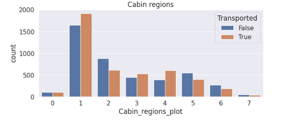
train['Cabin_regions_plot']=(train['Cabin_region1']+2*train['Cabin_region2']+3*train['Cabin_region3']+4*train['Cabin_region4']+5*train['Cabin_region5']+6*train['Cabin_region6']+7*train['Cabin_region7']).astype(int)
sns.countplot(data=train, x='Cabin_regions_plot', hue='Transported')
plt.title('Cabin regions')
train.drop('Cabin_regions_plot', axis=1, inplace=True)
(4)根据Name的姓氏划分出家庭组
根据形式划分出家庭组,再根据家庭组的大小划分出一个新的二元属性。
# 现在用离群值替换NaN(这样我们就可以拆分特征)
train['Name'].fillna('Unknown Unknown', inplace=True)
test['Name'].fillna('Unknown Unknown', inplace=True)# 新特征-姓氏
train['Surname']=train['Name'].str.split().str[-1]
test['Surname']=test['Name'].str.split().str[-1]# 新特征-家庭大小
train['Family_size']=train['Surname'].map(lambda x: pd.concat([train['Surname'],test['Surname']]).value_counts()[x])
test['Family_size']=test['Surname'].map(lambda x: pd.concat([train['Surname'],test['Surname']]).value_counts()[x])# 把Nan的放回去(我们稍后会填充这些)
train.loc[train['Surname']=='Unknown','Surname']=np.nan
train.loc[train['Family_size']>100,'Family_size']=np.nan
test.loc[test['Surname']=='Unknown','Surname']=np.nan
test.loc[test['Family_size']>100,'Family_size']=np.nan# 删除Name(我们不再需要它了)
train.drop('Name', axis=1, inplace=True)
test.drop('Name', axis=1, inplace=True)# 新特征分布图
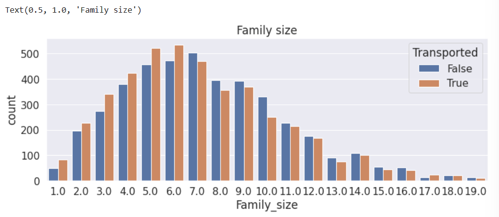
plt.figure(figsize=(12,4))
sns.countplot(data=train, x='Family_size', hue='Transported')
plt.title('Family size')
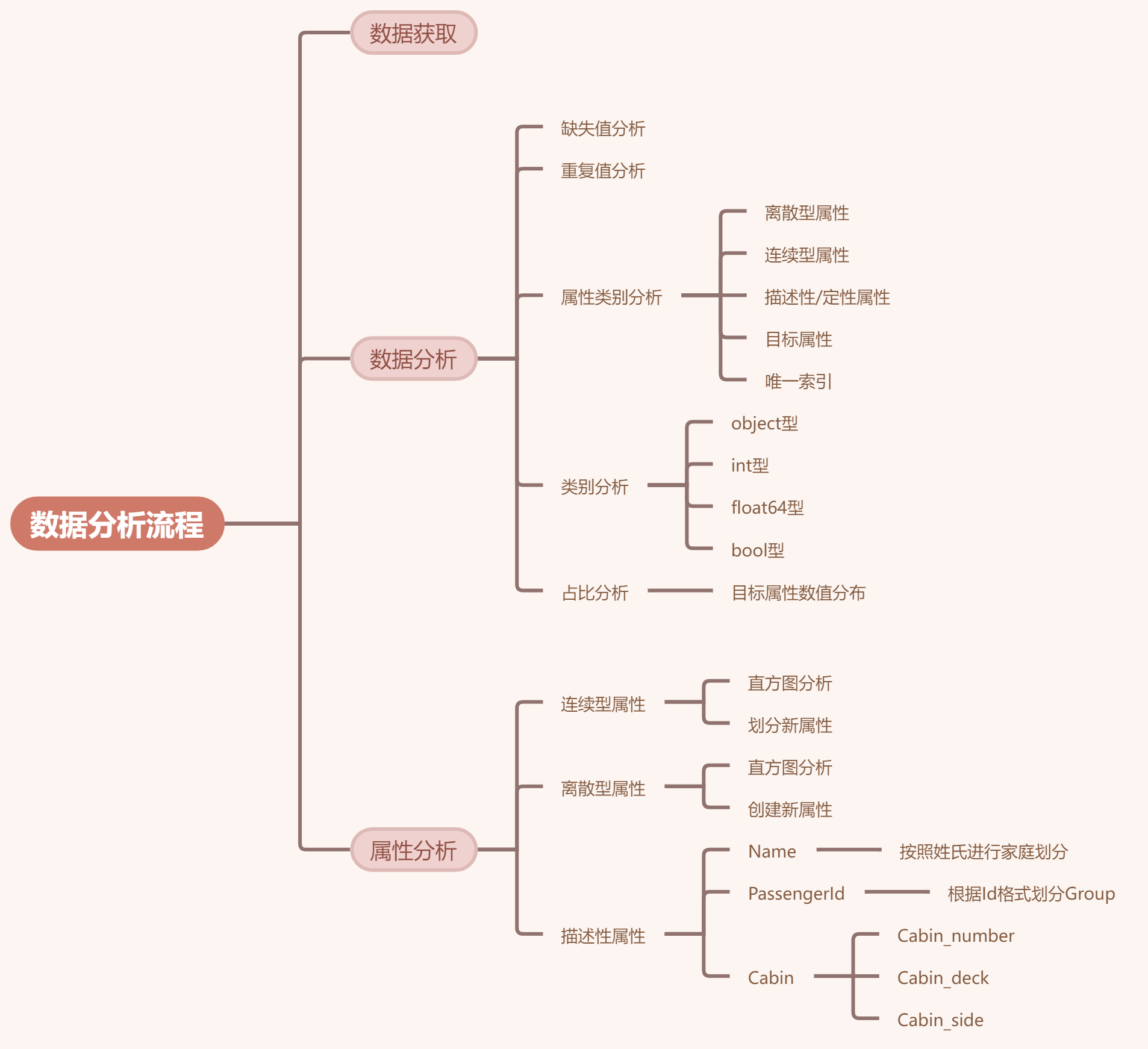
(四)归纳总结
数据分析流程总结
(五)写在最后
至此,我们已经完成了对数据集的初步分析,下一篇我们会对该数据集进行预处理。
Kaggle竞赛系列_SpaceshipTitanic金牌方案分析_数据处理
相关文章:
Kaggle竞赛系列_SpaceshipTitanic金牌方案分析_数据分析
文章目录 【文章系列】【前言】【比赛简介】【正文】(一)数据获取(二)数据分析1. 缺失值2. 重复值3. 属性类型分析4. 类别分析5. 分析目标数值占比 (三)属性分析1. 对年龄Age分析(1)…...
Tortoise-tts Better speech synthesis through scaling——TTS论文阅读
笔记地址:https://flowus.cn/share/a79f6286-b48f-42be-8425-2b5d0880c648 【FlowUs 息流】tortoise 论文地址: Better speech synthesis through scaling Abstract: 自回归变换器和DDPM:自回归变换器(autoregressive transfo…...

单元测试工具JEST入门——纯函数的测试
单元测试工具JEST入门——纯函数的测试 什么是测试❓🙉 我只是开发而已?常见单元测试工具 🔧jest的使用👀 首先你得知道一个简单的例子🌰😨 Oops!出现了一些问题👏 高效的持续监听&a…...
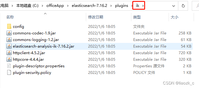
Elasticsearch Windows版安装配置
Elasticsearch简介 Elasticsearch是一个开源的搜索文献的引擎,大概含义就是你通过Rest请求告诉它关键字,他给你返回对应的内容,就这么简单。 Elasticsearch封装了Lucene,Lucene是apache软件基金会一个开放源代码的全文检索引擎工…...

安装 vant-ui 实现底部导航栏 Tabbar
本例子使用vue3 介绍 vant-ui 地址:介绍 - Vant 4 (vant-ui.github.io) Vant 是一个轻量、可定制的移动端组件库 安装 通过 npm 安装: # Vue 3 项目,安装最新版 Vant npm i vant # Vue 2 项目,安装 Vant 2 npm i vantlatest-v…...

GitHub国内打不开(解决办法有效)
最近国内访问github.com经常打不开,无法访问。 github网站打不开的解决方法 1.打开网站http://tool.chinaz.com/dns/ ,在A类型的查询中输入 github.com,找出最快的IP地址。 2.修改hosts文件。 在hosts文件中添加: # localhost n…...

Unity之第一人称角色控制
目录 第一人称角色控制 😴1、准备工作 📺2、鼠标控制摄像机视角 🎮3、角色控制 😃4.杂谈 第一人称角色控制 专栏Unity之动画和角色控制-CSDN博客的这一篇也有讲到角色控制器,是第三人称视角的,以小编…...
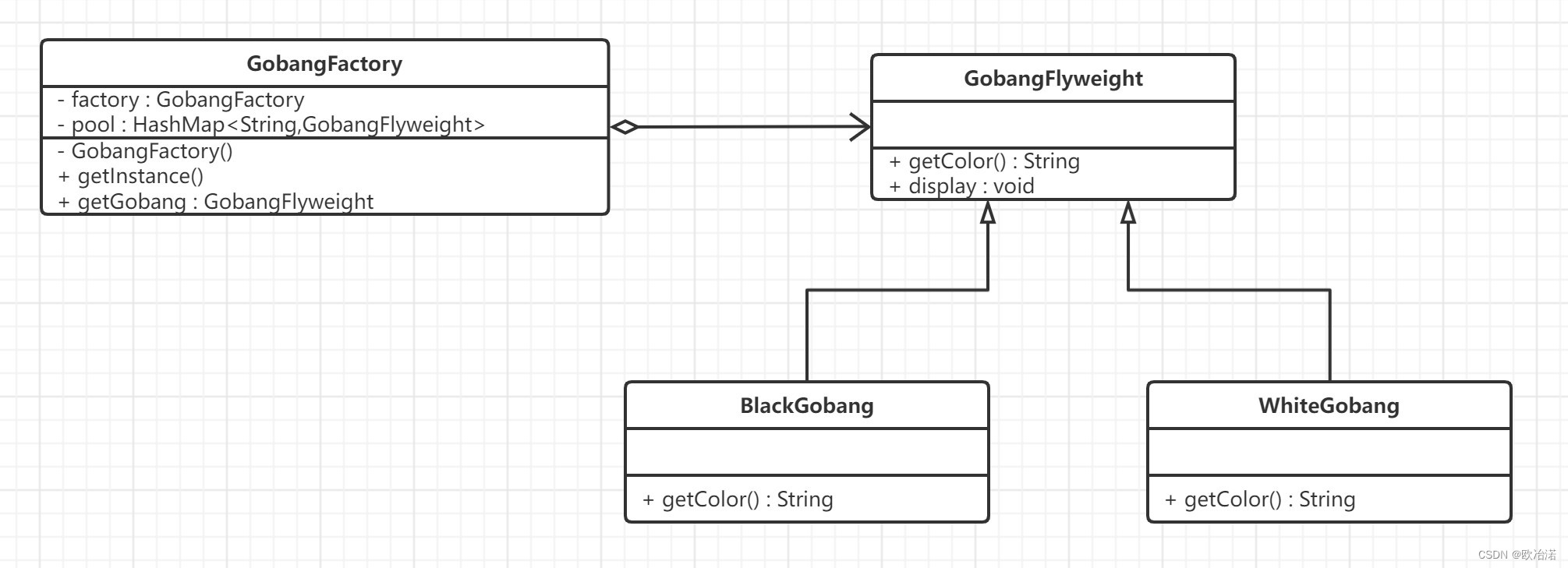
23种设计模式-结构型模式
1.代理模式 在软件开发中,由于一些原因,客户端不想或不能直接访问一个对象,此时可以通过一个称为"代理"的第三者来实现间接访问.该方案对应的设计模式被称为代理模式. 代理模式(Proxy Design Pattern ) 原始定义是:让你能够提供对象的替代品或其占位符。…...

python -- 流程控制
1、if控制语句:语法格式: age 20 if age > 18:print("我不是小孩子") elif age < 18:print("你永远都是小孩子") else:print("你永远都是小孩子") 2、while循环语句:语法格式: age1 30 …...
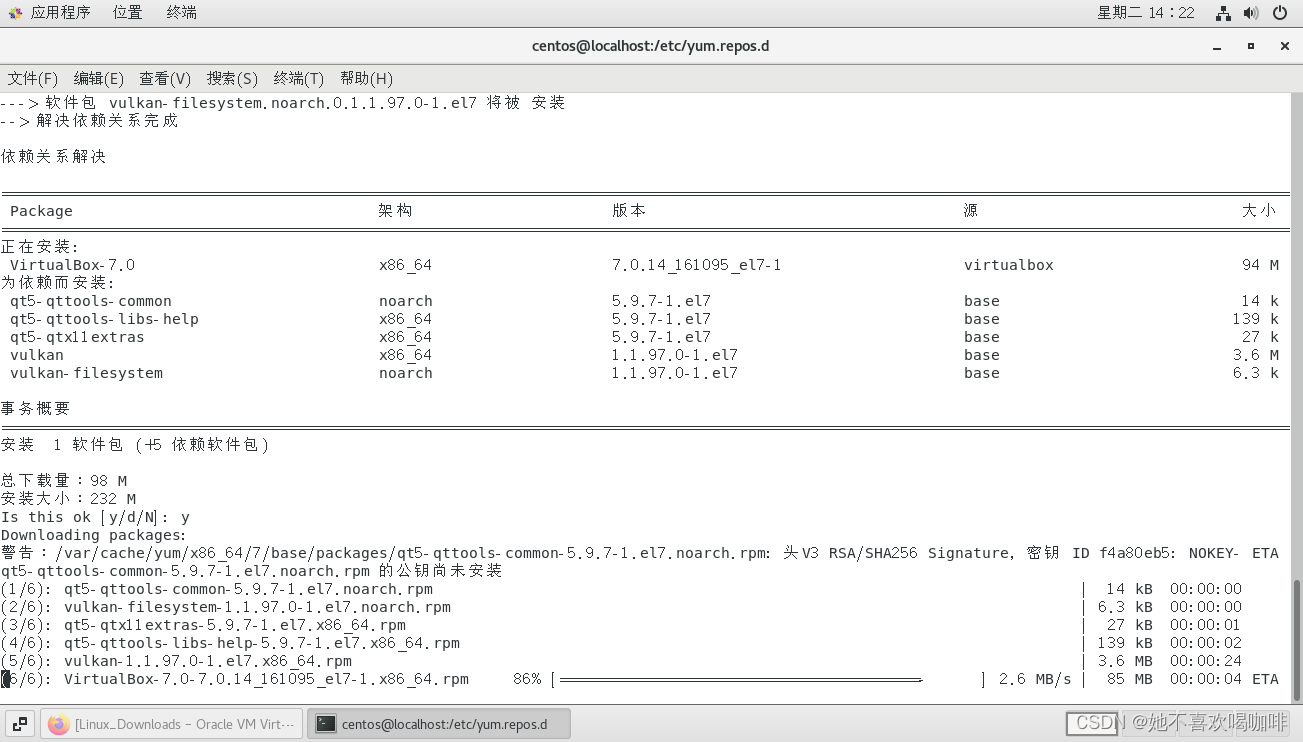
Centos 7.9 在线安装 VirtualBox 7.0
1 访问 Linux_Downloads – Oracle VM VirtualBox 2 点击 the Oracle Linux repo file 复制 内容到 /etc/yum.repos.d/. 3 在 /etc/yum.repos.d/ 目录下新建 virtualbox.repo,复制内容到 virtualbox.repo 并 :wq 保存。 [rootlocalhost centos]# cd /etc/yum.rep…...
mysql之基本查询
基本查询 一、SELECT 查询语句 一、SELECT 查询语句 查询所有列 1 SELECT *FORM emp;查询指定字段 SELECT empno,ename,job FROM emp;给字段取别名 SELECT empno 员工编号 FROM emp; SELECT empno 员工编号,ename 姓名,job 岗位 FROM emp; SELECT empno AS 员工编号,ename …...

鸿蒙(HarmonyOS)项目方舟框架(ArkUI)之DataPanel组件
鸿蒙(HarmonyOS)项目方舟框架(ArkUI)之DataPanel组件 一、操作环境 操作系统: Windows 10 专业版、IDE:DevEco Studio 3.1、SDK:HarmonyOS 3.1 二、DataPanel组件 数据面板组件,用于将多个数据占比情况使用占比图进…...
qt5-入门
参考: qt学习指南 Qt5和Qt6的区别-CSDN博客 Qt 学习之路_w3cschool Qt教程,Qt5编程入门教程(非常详细) 本地环境: win10专业版,64位 技术选择 Qt5力推QML界面编程。QML类似HTML,可以借助CSS进…...

【重磅发布】已开放!模型师入驻、转格式再升级、3D展示框架全新玩法…
1月23日,老子云正式发布全新版本。此次新版本包含多板块功能上线和升级,为用户带来了含模型师入驻、三维格式在线转换升级、模型免费增值权益开放、全新3D展示框架等一系列精彩内容! 1月23日,老子云正式发布全新版本。此次新版本…...

Qt 基础之QDataTime
Qt 基础之QDataTime 引言一、获取(设定)日期和时间二、时间戳三、时间计算 (重载运算符) 引言 QDataTime是Qt框架中用于处理日期和时间的类。它提供了操作和格式化日期、时间和日期时间组合的功能。QDataTime可以用于存储和检索日期和时间、比较日期和时间、对日期和时间执行算…...
美国将限制中国,使用Azure、AWS等云,训练AI大模型
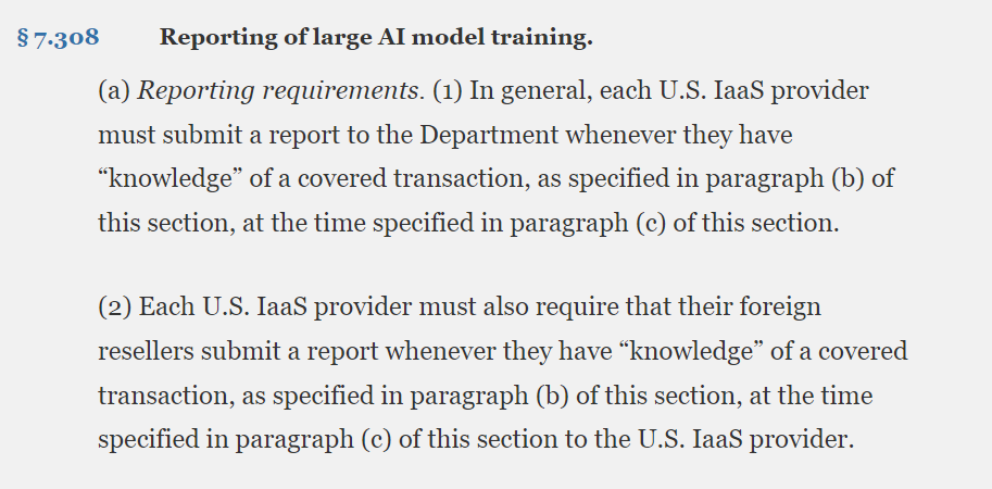
1月29日,美国商务部在Federal Register(联邦公报)正式公布了,《采取额外措施应对与重大恶意网络行为相关的国家紧急状态》提案。 该提案明确要求美国IaaS(云服务)厂商在提供云服务时,要验证外国…...

智能指针|巨巨巨详细
智能指针 shared_ptrshared_ptr的基本用法使用shared_ptr要注意的问题 unique_ptr独占的智能指针weak_ptr弱引用的智能指针weak_ptr的基本用法weak_ptr返回this指针weak_ptr解决循环引用问题 weak_ptr使用注意事项 智能指针 C程序设计中使用堆内存是非常频繁的操作࿰…...

硬件知识(2) 手机的传感器-sensor
#灵感# 看看小米在干啥 手机型号:Redmi Note 13 Pro,解读一下它宣传的手机卖点。 目录 宣传1:1/1.4" 大底,f/1.65 大光圈, 宣传2:支持 2 亿像素超清直出,分辨率高达 16320 x 12240 宣…...
Kotlin快速入门系列9
Kotlin对象表达式和对象声明 对象表达式 有时,我们想要创建一个对当前类有些许修改的对象同时又不想重新声明一个子类。如果是Java,可以用匿名内部类的概念来解决这个问题。kotlin的对象表达式和对象声明就是为了实现这一点(创建一个对某个类做了轻微改…...
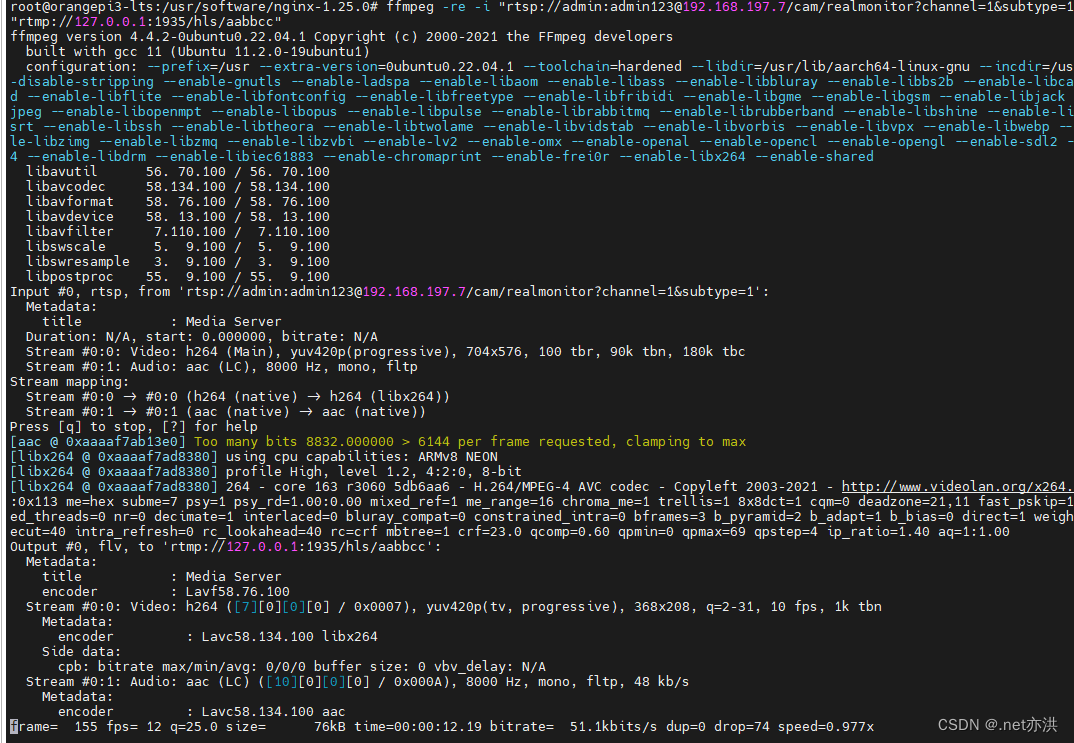
nginx+nginx-rtmp-module+ffmpeg进行局域网推流rtmp\m3u8
局域网推流的简单方式 这里以ubuntu为例 一、先下载安装包 nginx、nginx-rtmp-module,再一起安装 # 下载nginx # 这里我安装的是 nginx-1.10.3 版本 cd /usr/software wget http://nginx.org/download/nginx-1.25.0.tar.gz tar -zxvf nginx-1.25.0.tar.gz# 下载ng…...

AI Agent 为什么必须有“记忆系统”?
导语:大模型不是没有智商,而是经常没有“记性”。真正能长期干活的 Agent,不是靠无限拉长上下文,而是靠一套会压缩、会检索、会遗忘、会治理的外置记忆系统。一、先给结论:Agent 的记忆系统,本质是“上下文…...

从脚本到系统:设计一个支持插件、限流、重试与监控的 Python 异步爬虫框架
从脚本到系统:设计一个支持插件、限流、重试与监控的 Python 异步爬虫框架 很多人第一次写 Python 爬虫,都是从几十行脚本开始的:requests.get()、BeautifulSoup、for 循环、保存 CSV。它很快,也很有成就感。但真实项目往往不是“…...

中兴新支点NewStartOS初体验:从激活到日常使用,聊聊这个国产Linux桌面的真实感受
中兴新支点NewStartOS深度体验:一个技术爱好者的真实使用笔记第一次启动中兴新支点NewStartOS时,那个简洁的登录界面就给我留下了不错的印象。作为一个长期在Windows和macOS之间切换的用户,这次尝试国产Linux桌面系统,更像是一次充…...

H.Test.DefaultApplicationBase-默认应用组合
H.Test.DefaultApplicationBase 示例项目学习教程 一、概述 H.Test.DefaultApplicationBase 展示了如何使用 WPF-Control 框架的默认应用组合(Default ApplicationBase)。这是一个"开箱即用"的应用模板,一键注册所有常用服务和模块…...

机器学习预测关税冲击下的股市波动:随机森林、SVR、kNN与线性回归实战对比
1. 项目概述与核心问题拆解做量化研究的朋友们,尤其是关注宏观事件对市场冲击的,应该都对“黑天鹅”事件不陌生。政策变动,特别是像关税这种直接影响国际贸易成本和公司利润的宏观变量,往往会在短期内引发市场剧烈波动。传统的做法…...

2026 最新版网络安全全岗位详解,入行择业一看就懂
全网最全!网络安全全岗位解析(2026版) 摘要:随着数字化转型加速,网络安全已成为企业、政务、互联网大厂的核心刚需,人才缺口持续扩大,2026年国内网络安全人才缺口已突破327万,全球缺…...

从‘调参苦手’到‘一击即中’:实战解读glmnet中lambda.min与lambda.1se到底怎么选
从‘调参苦手’到‘一击即中’:实战解读glmnet中lambda.min与lambda.1se到底怎么选 在机器学习的世界里,LASSO回归就像一位精明的裁缝,能够为数据量身定制最合身的模型。而glmnet包中的lambda.min和lambda.1se,则是这位裁缝手中的…...
(Google drive存储解密密钥,加密聊天记录还是存储在Meta服务器上)聊天加密)
Messenger端到端加密机制(end-to-end encryption)(Google drive存储解密密钥,加密聊天记录还是存储在Meta服务器上)聊天加密
Messenger有个save key in google drive选项,这是什么,是指把聊天记录存于google drive吗?还是只存一个key?只存一个key有啥用啊? 文章目录解释为什么只存 key 就够了?如果没有这个 key 会怎样?…...

5分钟学会使用Mermaid Live Editor:免费在线图表编辑器的完整指南
5分钟学会使用Mermaid Live Editor:免费在线图表编辑器的完整指南 【免费下载链接】mermaid-live-editor Edit, preview and share mermaid charts/diagrams. New implementation of the live editor. 项目地址: https://gitcode.com/GitHub_Trending/me/mermaid-…...
)
别再傻傻分不清!Keil C51和MDK-ARM双版本保姆级安装与共存指南(附资源)
Keil C51与MDK-ARM双版本高效共存实战手册 引言:为什么开发者需要同时安装两个版本? 在嵌入式开发领域,51单片机和ARM架构设备依然占据着重要地位。许多工程师和学生在项目开发或学习过程中,常常需要同时接触这两种不同架构的芯片…...