金融贷款批准预测项目
注意:本文引用自专业人工智能社区Venus AI
更多AI知识请参考原站 ([www.aideeplearning.cn])
在金融服务行业,贷款审批是一项关键任务,它不仅关系到资金的安全,还直接影响到金融机构的运营效率和风险管理。传统的审批流程往往依赖于人工审核,这不仅效率低下,而且容易受到主观判断的影响。为了解决这些问题,我们引入了一种基于机器学习的贷款预测模型,旨在提高贷款审批的准确性和效率。
项目背景
在当前的金融市场中,违约率的不断波动对贷款审批流程提出了新的挑战。传统方法往往无法有效预测和管理这些风险,因此需要一种更智能、更可靠的方法来评估贷款申请。通过使用机器学习,我们可以从大量历史数据中学习并识别违约的潜在风险,这不仅能提高贷款批准的准确性,还能大大降低金融机构的损失。
经过训练的模型将用于预测新的贷款申请是否有高风险。这将帮助金融机构在贷款批准过程中做出更加明智的决策,减少不良贷款的比例,提高整体的财务健康状况。
数据集
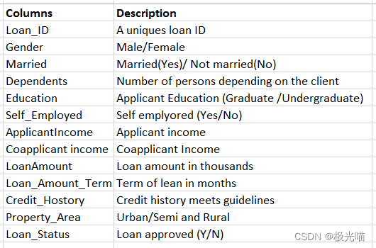
我们项目使用的数据集包括了广泛的客户特征,这些特征反映了贷款申请者的财务状况和背景。具体包括:
- 性别(Gender):申请人的性别。
- 婚姻状况(Married):申请人的婚姻状态。
- 受抚养人数(Dependents):申请人负责抚养的人数。
- 教育背景(Education):申请人的教育水平。
- 是否自雇(Self_Employed):申请人是否拥有自己的业务。
- 申请人收入(ApplicantIncome):申请人的月收入。
- 共同申请人收入(CoapplicantIncome):与申请人一同申请贷款的人的月收入。
- 贷款金额(LoanAmount):申请的贷款总额。
- 贷款期限(Loan_Amount_Term):预期的还款期限。
- 信用历史(Credit_History):申请人的信用记录。
- 财产区域(Property_Area):申请人财产所在的地理位置。
模型和依赖库
Models:
- RandomForestRegressor
- Decision Tree Regression
- logistic regression
Libraries:
- matplotlib==3.7.1
- numpy==1.24.3
- pandas==2.0.2
- scikit_learn==1.2.2
- seaborn==0.13.0
代码实现
金融贷款批准预测
项目背景
在金融领域,贷款审批是向任何人提供贷款之前需要执行的一项至关重要的任务。 这确保了批准的贷款将来可以收回。 然而,要确定一个人是否适合贷款或违约者,就很难确定有助于做出决定的性格和特征。
在这些情况下,使用机器学习的贷款预测模型成为非常有用的工具,可以根据过去的数据来预测该人是否违约。
我们获得了两个数据集(训练和测试),其中包含过去的交易,其中包括客户的一些特征以及显示客户是否违约的标签。 我们建立了一个模型,可以在训练数据集上执行,并可以预测贷款是否应获得批准。
About Data:
导入库并加载数据
#Impoting libraries
import pandas as pd
import numpy as np
import matplotlib.pyplot as plt
import seaborn as sns
df_train = pd.read_csv("train_u6lujuX_CVtuZ9i.csv")
df_test = pd.read_csv("test_Y3wMUE5_7gLdaTN.csv")df_train.head()| Loan_ID | Gender | Married | Dependents | Education | Self_Employed | ApplicantIncome | CoapplicantIncome | LoanAmount | Loan_Amount_Term | Credit_History | Property_Area | Loan_Status | |
|---|---|---|---|---|---|---|---|---|---|---|---|---|---|
| 0 | LP001002 | Male | No | 0 | Graduate | No | 5849 | 0.0 | NaN | 360.0 | 1.0 | Urban | Y |
| 1 | LP001003 | Male | Yes | 1 | Graduate | No | 4583 | 1508.0 | 128.0 | 360.0 | 1.0 | Rural | N |
| 2 | LP001005 | Male | Yes | 0 | Graduate | Yes | 3000 | 0.0 | 66.0 | 360.0 | 1.0 | Urban | Y |
| 3 | LP001006 | Male | Yes | 0 | Not Graduate | No | 2583 | 2358.0 | 120.0 | 360.0 | 1.0 | Urban | Y |
| 4 | LP001008 | Male | No | 0 | Graduate | No | 6000 | 0.0 | 141.0 | 360.0 | 1.0 | Urban | Y |
df_test.head()| Loan_ID | Gender | Married | Dependents | Education | Self_Employed | ApplicantIncome | CoapplicantIncome | LoanAmount | Loan_Amount_Term | Credit_History | Property_Area | |
|---|---|---|---|---|---|---|---|---|---|---|---|---|
| 0 | LP001015 | Male | Yes | 0 | Graduate | No | 5720 | 0 | 110.0 | 360.0 | 1.0 | Urban |
| 1 | LP001022 | Male | Yes | 1 | Graduate | No | 3076 | 1500 | 126.0 | 360.0 | 1.0 | Urban |
| 2 | LP001031 | Male | Yes | 2 | Graduate | No | 5000 | 1800 | 208.0 | 360.0 | 1.0 | Urban |
| 3 | LP001035 | Male | Yes | 2 | Graduate | No | 2340 | 2546 | 100.0 | 360.0 | NaN | Urban |
| 4 | LP001051 | Male | No | 0 | Not Graduate | No | 3276 | 0 | 78.0 | 360.0 | 1.0 | Urban |
#shape of data
df_train.shape
(614, 13)
#data summary
df_train.describe()| ApplicantIncome | CoapplicantIncome | LoanAmount | Loan_Amount_Term | Credit_History | |
|---|---|---|---|---|---|
| count | 614.000000 | 614.000000 | 592.000000 | 600.00000 | 564.000000 |
| mean | 5403.459283 | 1621.245798 | 146.412162 | 342.00000 | 0.842199 |
| std | 6109.041673 | 2926.248369 | 85.587325 | 65.12041 | 0.364878 |
| min | 150.000000 | 0.000000 | 9.000000 | 12.00000 | 0.000000 |
| 25% | 2877.500000 | 0.000000 | 100.000000 | 360.00000 | 1.000000 |
| 50% | 3812.500000 | 1188.500000 | 128.000000 | 360.00000 | 1.000000 |
| 75% | 5795.000000 | 2297.250000 | 168.000000 | 360.00000 | 1.000000 |
| max | 81000.000000 | 41667.000000 | 700.000000 | 480.00000 | 1.000000 |
df_train.info()<class 'pandas.core.frame.DataFrame'> RangeIndex: 614 entries, 0 to 613 Data columns (total 13 columns):# Column Non-Null Count Dtype --- ------ -------------- ----- 0 Loan_ID 614 non-null object 1 Gender 601 non-null object 2 Married 611 non-null object 3 Dependents 599 non-null object 4 Education 614 non-null object 5 Self_Employed 582 non-null object 6 ApplicantIncome 614 non-null int64 7 CoapplicantIncome 614 non-null float648 LoanAmount 592 non-null float649 Loan_Amount_Term 600 non-null float6410 Credit_History 564 non-null float6411 Property_Area 614 non-null object 12 Loan_Status 614 non-null object dtypes: float64(4), int64(1), object(8) memory usage: 62.5+ KB
数据清洗
# 检测空值
df_train.isna().sum()
Loan_ID 0 Gender 13 Married 3 Dependents 15 Education 0 Self_Employed 32 ApplicantIncome 0 CoapplicantIncome 0 LoanAmount 22 Loan_Amount_Term 14 Credit_History 50 Property_Area 0 Loan_Status 0 dtype: int64
有很多空值,Credit_History 的最大值为 50。
去除所有空值
# Dropping all the null values
drop_list = ['Gender','Married','Dependents','Self_Employed','LoanAmount','Loan_Amount_Term','Credit_History']
for col in drop_list:df_train = df_train[~df_train[col].isna()]df_train.isna().sum()Loan_ID 0 Gender 0 Married 0 Dependents 0 Education 0 Self_Employed 0 ApplicantIncome 0 CoapplicantIncome 0 LoanAmount 0 Loan_Amount_Term 0 Credit_History 0 Property_Area 0 Loan_Status 0 dtype: int64
Loan_ID 列没用,这里删除它
# dropping Loan_ID
df_train.drop(columns='Loan_ID',axis=1, inplace=True)df_train.shape(480, 12)
#data summary
df_train.describe()| ApplicantIncome | CoapplicantIncome | LoanAmount | Loan_Amount_Term | Credit_History | |
|---|---|---|---|---|---|
| count | 480.000000 | 480.000000 | 480.000000 | 480.000000 | 480.000000 |
| mean | 5364.231250 | 1581.093583 | 144.735417 | 342.050000 | 0.854167 |
| std | 5668.251251 | 2617.692267 | 80.508164 | 65.212401 | 0.353307 |
| min | 150.000000 | 0.000000 | 9.000000 | 36.000000 | 0.000000 |
| 25% | 2898.750000 | 0.000000 | 100.000000 | 360.000000 | 1.000000 |
| 50% | 3859.000000 | 1084.500000 | 128.000000 | 360.000000 | 1.000000 |
| 75% | 5852.500000 | 2253.250000 | 170.000000 | 360.000000 | 1.000000 |
| max | 81000.000000 | 33837.000000 | 600.000000 | 480.000000 | 1.000000 |
数据分析(EDA)
df_train.head()| Gender | Married | Dependents | Education | Self_Employed | ApplicantIncome | CoapplicantIncome | LoanAmount | Loan_Amount_Term | Credit_History | Property_Area | Loan_Status | |
|---|---|---|---|---|---|---|---|---|---|---|---|---|
| 1 | Male | Yes | 1 | Graduate | No | 4583 | 1508.0 | 128.0 | 360.0 | 1.0 | Rural | N |
| 2 | Male | Yes | 0 | Graduate | Yes | 3000 | 0.0 | 66.0 | 360.0 | 1.0 | Urban | Y |
| 3 | Male | Yes | 0 | Not Graduate | No | 2583 | 2358.0 | 120.0 | 360.0 | 1.0 | Urban | Y |
| 4 | Male | No | 0 | Graduate | No | 6000 | 0.0 | 141.0 | 360.0 | 1.0 | Urban | Y |
| 5 | Male | Yes | 2 | Graduate | Yes | 5417 | 4196.0 | 267.0 | 360.0 | 1.0 | Urban | Y |
#distribution of Churn data
sns.displot(data=df_train,x='Loan_Status')
<seaborn.axisgrid.FacetGrid at 0x1f54d853bb0>
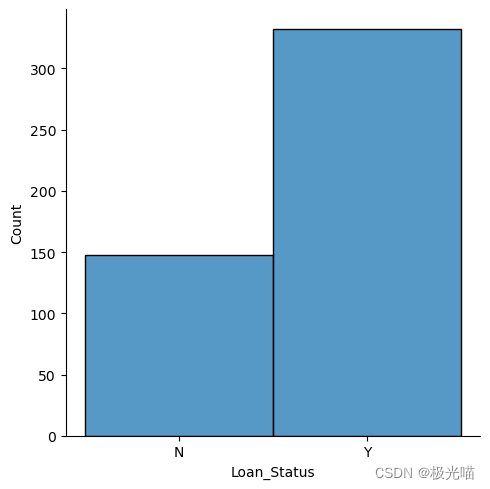
数据集是不平衡的,但是不是非常严重
自变量相对于因变量的分布.
# 设置分类特征
categorical_features=list(df_train.columns)
numeical_features = list(df_train.describe().columns)
for elem in numeical_features:categorical_features.remove(elem)
categorical_features = categorical_features[:-1]
categorical_features
['Gender','Married','Dependents','Education','Self_Employed','Property_Area']
# Set categorical and numerical features
categorical_features = list(df_train.columns)
numerical_features = list(df_train.describe().columns)
for elem in numerical_features:categorical_features.remove(elem)
categorical_features.remove('Loan_Status')  # Assuming 'Loan_Status' is not a feature to plot# Determine the layout of subplots
n_cols = 2  # Can be adjusted based on preference
n_rows = (len(categorical_features) + 1) // n_cols# Create a grid of subplots
fig, axes = plt.subplots(nrows=n_rows, ncols=n_cols, figsize=(12, n_rows * 4))# Flatten the axes array for easy iteration
axes = axes.flatten()# Plot each bar chart
for i, col in enumerate(categorical_features):df_train.groupby([col, 'Loan_Status']).size().unstack().plot(kind='bar', stacked=True, ax=axes[i])axes[i].set_title(f'Total count of Loan_Status grouped by {col}')axes[i].set_ylabel('Count')# Adjust layout and display the plot
plt.tight_layout()
plt.show()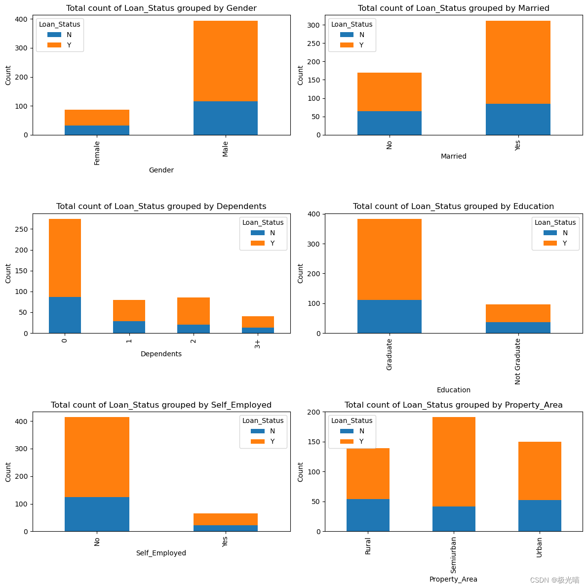
从上面的图中观察到的结果:
- 与女性相比,男性获得贷款批准的比例更高。
-
与非毕业生相比,贷款审批对毕业生更有利。
-
与受雇者相比,个体经营者获得贷款批准的机会较少。
- 城乡结合部的贷款批准率最高。
让我们看看按因变量分组的连续自变量
numerical_features = df_train.describe().columns# Determine the layout of subplots
n_cols = 2  # Adjust based on preference
n_rows = (len(numerical_features) + 1) // n_cols# Create a grid of subplots
fig, axes = plt.subplots(nrows=n_rows, ncols=n_cols, figsize=(12, n_rows * 4))# Flatten the axes array for easy iteration
axes = axes.flatten()# Plot each boxplot
for i, col in enumerate(numerical_features):sns.boxplot(x='Loan_Status', y=col, data=df_train, ax=axes[i])axes[i].set_title(f'Distribution of {col} grouped by Loan_Status')# Adjust layout and display the plot
plt.tight_layout()
plt.show()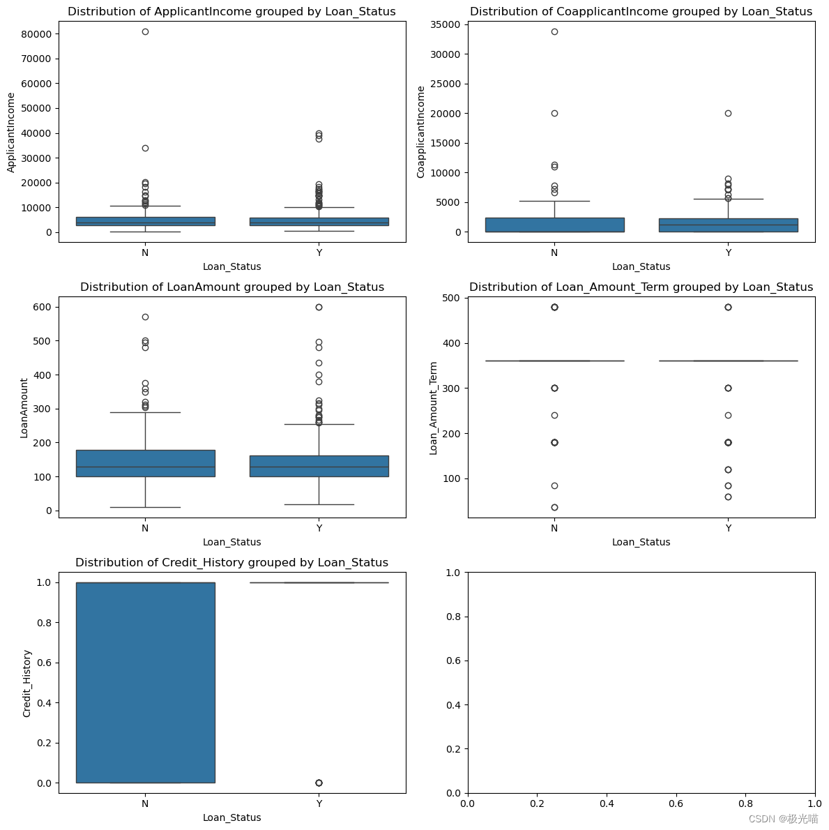
我们可以在数据中观察到很多异常值。
从上面的箱线图中无法得出任何正确的结论。
相关性分析
 ## Correlation between variables
plt.figure(figsize=(15,8))
correlation = df_train.corr()
sns.heatmap((correlation), annot=True, cmap='coolwarm')
<Axes: >

没有观察到任何显着的相关性。
数据预处理
df_train.head()| Gender | Married | Dependents | Education | Self_Employed | ApplicantIncome | CoapplicantIncome | LoanAmount | Loan_Amount_Term | Credit_History | Property_Area | Loan_Status | |
|---|---|---|---|---|---|---|---|---|---|---|---|---|
| 1 | Male | Yes | 1 | Graduate | No | 4583 | 1508.0 | 128.0 | 360.0 | 1.0 | Rural | N |
| 2 | Male | Yes | 0 | Graduate | Yes | 3000 | 0.0 | 66.0 | 360.0 | 1.0 | Urban | Y |
| 3 | Male | Yes | 0 | Not Graduate | No | 2583 | 2358.0 | 120.0 | 360.0 | 1.0 | Urban | Y |
| 4 | Male | No | 0 | Graduate | No | 6000 | 0.0 | 141.0 | 360.0 | 1.0 | Urban | Y |
| 5 | Male | Yes | 2 | Graduate | Yes | 5417 | 4196.0 | 267.0 | 360.0 | 1.0 | Urban | Y |
df_train['Property_Area'].value_counts()Semiurban 191 Urban 150 Rural 139 Name: Property_Area, dtype: int64
df_train['Credit_History'].value_counts()1.0 410 0.0 70 Name: Credit_History, dtype: int64
df_train['Dependents'].value_counts()0 274 2 85 1 80 3+ 41 Name: Dependents, dtype: int64
使用标签编码将分类列转换为数字
#Label encoding for some categorical features
df_train_new = df_train.copy()
label_col_list = ['Married','Self_Employed']
for col in label_col_list:df_train_new=df_train_new.replace({col:{'Yes':1,'No':0}})
df_train_new=df_train_new.replace({'Gender':{'Male':1,'Female':0}})
df_train_new=df_train_new.replace({'Education':{'Graduate':1,'Not Graduate':0}})
df_train_new=df_train_new.replace({'Loan_Status':{'Y':1,'N':0}})对于其余的分类特征,我们将进行一种热编码:
#one hot encoding
df_train_new = pd.get_dummies(df_train_new, columns=["Dependents","Property_Area"])df_train_new.head()| Gender | Married | Education | Self_Employed | ApplicantIncome | CoapplicantIncome | LoanAmount | Loan_Amount_Term | Credit_History | Loan_Status | Dependents_0 | Dependents_1 | Dependents_2 | Dependents_3+ | Property_Area_Rural | Property_Area_Semiurban | Property_Area_Urban | |
|---|---|---|---|---|---|---|---|---|---|---|---|---|---|---|---|---|---|
| 1 | 1 | 1 | 1 | 0 | 4583 | 1508.0 | 128.0 | 360.0 | 1.0 | 0 | 0 | 1 | 0 | 0 | 1 | 0 | 0 |
| 2 | 1 | 1 | 1 | 1 | 3000 | 0.0 | 66.0 | 360.0 | 1.0 | 1 | 1 | 0 | 0 | 0 | 0 | 0 | 1 |
| 3 | 1 | 1 | 0 | 0 | 2583 | 2358.0 | 120.0 | 360.0 | 1.0 | 1 | 1 | 0 | 0 | 0 | 0 | 0 | 1 |
| 4 | 1 | 0 | 1 | 0 | 6000 | 0.0 | 141.0 | 360.0 | 1.0 | 1 | 1 | 0 | 0 | 0 | 0 | 0 | 1 |
| 5 | 1 | 1 | 1 | 1 | 5417 | 4196.0 | 267.0 | 360.0 | 1.0 | 1 | 0 | 0 | 1 | 0 | 0 | 0 | 1 |
标准化连续变量。
#standardize continuous features
from scipy.stats import zscore
df_train_new[['ApplicantIncome','CoapplicantIncome','LoanAmount','Loan_Amount_Term']]=df_train_new[['ApplicantIncome','CoapplicantIncome','LoanAmount','Loan_Amount_Term']].apply(zscore) df_train_new.head()| Gender | Married | Education | Self_Employed | ApplicantIncome | CoapplicantIncome | LoanAmount | Loan_Amount_Term | Credit_History | Loan_Status | Dependents_0 | Dependents_1 | Dependents_2 | Dependents_3+ | Property_Area_Rural | Property_Area_Semiurban | Property_Area_Urban | |
|---|---|---|---|---|---|---|---|---|---|---|---|---|---|---|---|---|---|
| 1 | 1 | 1 | 1 | 0 | -0.137970 | -0.027952 | -0.208089 | 0.275542 | 1.0 | 0 | 0 | 1 | 0 | 0 | 1 | 0 | 0 |
| 2 | 1 | 1 | 1 | 1 | -0.417536 | -0.604633 | -0.979001 | 0.275542 | 1.0 | 1 | 1 | 0 | 0 | 0 | 0 | 0 | 1 |
| 3 | 1 | 1 | 0 | 0 | -0.491180 | 0.297100 | -0.307562 | 0.275542 | 1.0 | 1 | 1 | 0 | 0 | 0 | 0 | 0 | 1 |
| 4 | 1 | 0 | 1 | 0 | 0.112280 | -0.604633 | -0.046446 | 0.275542 | 1.0 | 1 | 1 | 0 | 0 | 0 | 0 | 0 | 1 |
| 5 | 1 | 1 | 1 | 1 | 0.009319 | 0.999978 | 1.520245 | 0.275542 | 1.0 | 1 | 0 | 0 | 1 | 0 | 0 | 0 | 1 |
# Repositioning the dependent variable to last index
last_column = df_train_new.pop('Loan_Status')
df_train_new.insert(16, 'Loan_Status', last_column)
df_train_new.head()| Gender | Married | Education | Self_Employed | ApplicantIncome | CoapplicantIncome | LoanAmount | Loan_Amount_Term | Credit_History | Dependents_0 | Dependents_1 | Dependents_2 | Dependents_3+ | Property_Area_Rural | Property_Area_Semiurban | Property_Area_Urban | Loan_Status | |
|---|---|---|---|---|---|---|---|---|---|---|---|---|---|---|---|---|---|
| 1 | 1 | 1 | 1 | 0 | -0.137970 | -0.027952 | -0.208089 | 0.275542 | 1.0 | 0 | 1 | 0 | 0 | 1 | 0 | 0 | 0 |
| 2 | 1 | 1 | 1 | 1 | -0.417536 | -0.604633 | -0.979001 | 0.275542 | 1.0 | 1 | 0 | 0 | 0 | 0 | 0 | 1 | 1 |
| 3 | 1 | 1 | 0 | 0 | -0.491180 | 0.297100 | -0.307562 | 0.275542 | 1.0 | 1 | 0 | 0 | 0 | 0 | 0 | 1 | 1 |
| 4 | 1 | 0 | 1 | 0 | 0.112280 | -0.604633 | -0.046446 | 0.275542 | 1.0 | 1 | 0 | 0 | 0 | 0 | 0 | 1 | 1 |
| 5 | 1 | 1 | 1 | 1 | 0.009319 | 0.999978 | 1.520245 | 0.275542 | 1.0 | 0 | 0 | 1 | 0 | 0 | 0 | 1 | 1 |
数据处理完毕,准备训练模型
数据集划分
由于我们的数据仅用于训练,其他数据可用于测试。 我们仍然会进行训练测试分割,因为测试数据没有标记,并且有必要根据未见过的数据评估模型。
X= df_train_new.iloc[:,:-1]
y= df_train_new.iloc[:,-1]
from sklearn.model_selection import train_test_split
X_train, X_test, y_train, y_test = train_test_split( X,y , test_size = 0.2, random_state = 0)
print(X_train.shape)
print(X_test.shape)
(384, 16) (96, 16)
y_train.value_counts()1 271 0 113 Name: Loan_Status, dtype: int64
y_test.value_counts()1 61 0 35 Name: Loan_Status, dtype: int64
对训练数据进行逻辑回归拟合
#Importing and fitting Logistic regression
from sklearn.linear_model import LogisticRegressionlr = LogisticRegression(fit_intercept=True, max_iter=10000,random_state=0)
lr.fit(X_train, y_train)
LogisticRegression
LogisticRegression(max_iter=10000, random_state=0)
# Get the model coefficients
lr.coef_
array([[ 0.23272114, 0.57128602, 0.26384918, -0.24617035, 0.15924191,-0.14703758, -0.19280038, -0.16392914, 2.97399665, -0.18202629,-0.27741114, 0.17256535, 0.28601466, -0.30275813, 0.64592912,-0.3440284 ]])
#model intercept
lr.intercept_
array([-2.1943974])
评价训练模型的性能
# Get the predicted probabilities
train_preds = lr.predict_proba(X_train)
test_preds = lr.predict_proba(X_test)test_predsarray([[0.23916396, 0.76083604],[0.24506751, 0.75493249],[0.04933527, 0.95066473],[0.20146124, 0.79853876],[0.2347122 , 0.7652878 ],[0.05817427, 0.94182573],[0.17668886, 0.82331114],[0.21352909, 0.78647091],[0.39015173, 0.60984827],[0.1902079 , 0.8097921 ],[0.20590091, 0.79409909],[0.184445 , 0.815555 ],[0.80677694, 0.19322306],[0.23024539, 0.76975461],[0.23674387, 0.76325613],[0.32409412, 0.67590588],[0.08612609, 0.91387391],[0.20502754, 0.79497246],[0.71006169, 0.28993831],[0.05818474, 0.94181526],[0.16546532, 0.83453468],[0.1191243 , 0.8808757 ],[0.16412334, 0.83587666],[0.14471253, 0.85528747],[0.49082632, 0.50917368],[0.37484189, 0.62515811],[0.20042593, 0.79957407],[0.07289182, 0.92710818],[0.10696878, 0.89303122],[0.27313905, 0.72686095],[0.07661587, 0.92338413],[0.07911086, 0.92088914],[0.32357856, 0.67642144],[0.24855278, 0.75144722],[0.25736849, 0.74263151],[0.10330185, 0.89669815],[0.27934665, 0.72065335],[0.23504431, 0.76495569],[0.37235234, 0.62764766],[0.82612173, 0.17387827],[0.25597195, 0.74402805],[0.07027974, 0.92972026],[0.21138903, 0.78861097],[0.30656929, 0.69343071],[0.12859877, 0.87140123],[0.22422238, 0.77577762],[0.19222405, 0.80777595],[0.33904961, 0.66095039],[0.21169609, 0.78830391],[0.12783677, 0.87216323],[0.21562742, 0.78437258],[0.1003408 , 0.8996592 ],[0.39205576, 0.60794424],[0.10298106, 0.89701894],[0.34917087, 0.65082913],[0.31848606, 0.68151394],[0.46697536, 0.53302464],[0.83005638, 0.16994362],[0.84749511, 0.15250489],[0.82240763, 0.17759237],[0.08938059, 0.91061941],[0.38214865, 0.61785135],[0.62202628, 0.37797372],[0.1124887 , 0.8875113 ],[0.29371977, 0.70628023],[0.12829643, 0.87170357],[0.30152976, 0.69847024],[0.12669798, 0.87330202],[0.07601492, 0.92398508],[0.06068026, 0.93931974],[0.05461916, 0.94538084],[0.10209121, 0.89790879],[0.20592351, 0.79407649],[0.56190874, 0.43809126],[0.19828342, 0.80171658],[0.20171019, 0.79828981],[0.11960918, 0.88039082],[0.25602438, 0.74397562],[0.18013843, 0.81986157],[0.37225288, 0.62774712],[0.21781716, 0.78218284],[0.10365239, 0.89634761],[0.29076172, 0.70923828],[0.59602673, 0.40397327],[0.39435357, 0.60564643],[0.40070233, 0.59929767],[0.88224869, 0.11775131],[0.22235351, 0.77764649],[0.1765423 , 0.8234577 ],[0.75247369, 0.24752631],[0.20366031, 0.79633969],[0.85207477, 0.14792523],[0.3873617 , 0.6126383 ],[0.12318258, 0.87681742],[0.06667711, 0.93332289],[0.17440779, 0.82559221]])
# Get the predicted classes
train_class_preds = lr.predict(X_train)
test_class_preds = lr.predict(X_test)train_class_predsarray([1, 1, 1, 1, 1, 1, 1, 1, 1, 1, 0, 1, 1, 1, 1, 1, 0, 1, 1, 1, 1, 1,0, 1, 1, 1, 1, 1, 1, 0, 1, 0, 1, 1, 1, 1, 1, 1, 1, 1, 1, 1, 1, 1,1, 1, 0, 1, 1, 1, 1, 1, 1, 1, 1, 1, 1, 1, 1, 0, 0, 1, 1, 1, 1, 1,1, 1, 0, 0, 1, 0, 1, 1, 1, 1, 1, 1, 1, 1, 0, 0, 0, 1, 1, 1, 1, 1,1, 1, 1, 1, 1, 0, 1, 1, 1, 1, 1, 1, 1, 0, 1, 1, 0, 0, 1, 1, 1, 1,1, 1, 1, 1, 1, 1, 1, 1, 1, 1, 1, 1, 0, 1, 1, 1, 1, 1, 1, 1, 1, 1,1, 1, 1, 1, 1, 1, 1, 0, 1, 1, 0, 1, 1, 1, 1, 1, 1, 1, 1, 1, 1, 1,0, 0, 0, 1, 1, 1, 0, 1, 1, 1, 1, 1, 1, 0, 1, 0, 1, 1, 1, 1, 1, 1,1, 1, 1, 1, 1, 1, 1, 1, 1, 1, 1, 1, 1, 1, 1, 1, 1, 1, 1, 1, 1, 0,1, 1, 1, 1, 1, 1, 1, 1, 0, 1, 1, 1, 0, 1, 1, 1, 0, 1, 1, 1, 1, 1,1, 1, 1, 1, 1, 1, 1, 1, 0, 1, 1, 1, 1, 1, 1, 1, 1, 1, 1, 0, 1, 1,1, 1, 1, 1, 1, 1, 1, 1, 0, 1, 0, 1, 1, 1, 1, 1, 1, 1, 0, 0, 1, 1,1, 1, 0, 1, 1, 1, 1, 1, 1, 1, 1, 1, 0, 1, 1, 1, 1, 1, 1, 1, 1, 1,1, 1, 1, 1, 1, 1, 1, 0, 1, 1, 1, 1, 0, 1, 1, 0, 1, 1, 1, 1, 1, 1,1, 1, 1, 0, 1, 1, 1, 1, 1, 1, 1, 0, 0, 1, 0, 1, 1, 1, 0, 1, 1, 1,1, 1, 1, 1, 1, 1, 1, 1, 1, 1, 0, 1, 1, 1, 1, 1, 1, 1, 0, 0, 1, 1,0, 0, 1, 1, 1, 1, 1, 0, 1, 1, 1, 1, 1, 1, 1, 1, 1, 1, 1, 1, 1, 0,1, 1, 1, 0, 1, 0, 1, 1, 1, 0], dtype=int64)
准确率
from sklearn.metrics import accuracy_score, confusion_matrix ,classification_report
# Get the accuracy scores
train_accuracy = accuracy_score(train_class_preds,y_train)
test_accuracy = accuracy_score(test_class_preds,y_test)print("The accuracy on train data is ", train_accuracy)
print("The accuracy on test data is ", test_accuracy)
The accuracy on train data is 0.8229166666666666 The accuracy on test data is 0.7604166666666666
由于我们的数据有些不平衡,准确性可能不是一个好的指标。 让我们使用 roc_auc 分数。
# Get the roc_auc scores
train_roc_auc = accuracy_score(y_train,train_class_preds)
test_roc_auc = accuracy_score(y_test,test_class_preds)print("The accuracy on train data is ", train_roc_auc)
print("The accuracy on test data is ", test_roc_auc)
The accuracy on train data is 0.8229166666666666 The accuracy on test data is 0.7604166666666666
# Other evaluation metrics for train data
print(classification_report(train_class_preds,y_train))
precision recall f1-score support0 0.45 0.89 0.60 571 0.98 0.81 0.89 327accuracy 0.82 384macro avg 0.71 0.85 0.74 384 weighted avg 0.90 0.82 0.84 384
# Other evaluation metrics for train data
print(classification_report(y_test,test_class_preds))
precision recall f1-score support0 1.00 0.34 0.51 351 0.73 1.00 0.84 61accuracy 0.76 96macro avg 0.86 0.67 0.68 96 weighted avg 0.83 0.76 0.72 96
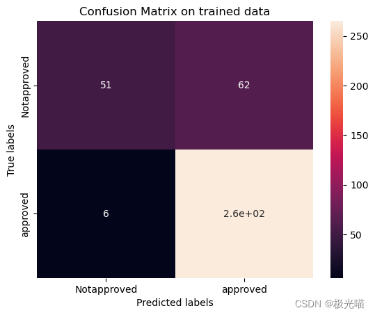
训练集和测试集上的混淆矩阵
# Get the confusion matrix for trained datalabels = ['Notapproved', 'approved']
cm = confusion_matrix(y_train, train_class_preds)
print(cm)ax= plt.subplot()
sns.heatmap(cm, annot=True, ax = ax) #annot=True to annotate cells# labels, title and ticks
ax.set_xlabel('Predicted labels')
ax.set_ylabel('True labels')
ax.set_title('Confusion Matrix on trained data')
ax.xaxis.set_ticklabels(labels)
ax.yaxis.set_ticklabels(labels)
plt.show()# Get the confusion matrix for test datalabels = ['Notapproved', 'approved']
cm = confusion_matrix(y_test, test_class_preds)
print(cm)ax= plt.subplot()
sns.heatmap(cm, annot=True, ax = ax); #annot=True to annotate cells# labels, title and ticks
ax.set_xlabel('Predicted labels')
ax.set_ylabel('True labels')
ax.set_title('Confusion Matrix on test data')
ax.xaxis.set_ticklabels(labels)
ax.yaxis.set_ticklabels(labels)
[[ 51 62][ 6 265]]
[[12 23][ 0 61]]
[Text(0, 0.5, 'Notapproved'), Text(0, 1.5, 'approved')]

决策树
#Importing libraries
from sklearn.tree import DecisionTreeClassifier
from sklearn.model_selection import GridSearchCV
# applying GreadsearchCV to identify best parameters
decision_tree = DecisionTreeClassifier()
tree_para = {'criterion':['gini','entropy'],'max_depth':[4,5,6,7,8,9,10,11,12,15,20,30,40,50,70,90,120,150]}
clf = GridSearchCV(decision_tree, tree_para, cv=5)
clf.fit(X_train, y_train)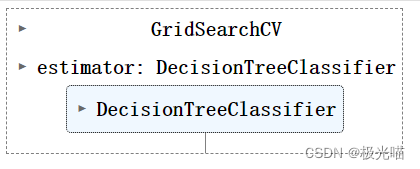
clf.best_params_{'criterion': 'gini', 'max_depth': 4}
#applying decision tree classifier
dt = DecisionTreeClassifier(criterion='gini',max_depth=4,random_state=0)
dt.fit(X_train, y_train)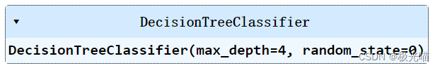
train_class_preds = dt.predict(X_train)
test_class_preds = dt.predict(X_test)
Accuracy Score
# Get the accuracy scores
train_accuracy = accuracy_score(train_class_preds,y_train)
test_accuracy = accuracy_score(test_class_preds,y_test)print("The accuracy on train data is ", train_accuracy)
print("The accuracy on test data is ", test_accuracy)
The accuracy on train data is 0.8463541666666666 The accuracy on test data is 0.71875
roc_auc score
# Get the roc_auc scores
train_roc_auc = accuracy_score(y_train,train_class_preds)
test_roc_auc = accuracy_score(y_test,test_class_preds)print("The accuracy on train data is ", train_roc_auc)
print("The accuracy on test data is ", test_roc_auc)
The accuracy on train data is 0.8463541666666666 The accuracy on test data is 0.71875
# Other evaluation metrics for train data
print(classification_report(train_class_preds,y_train))
precision recall f1-score support0 0.54 0.90 0.67 681 0.97 0.84 0.90 316accuracy 0.85 384macro avg 0.76 0.87 0.79 384 weighted avg 0.90 0.85 0.86 384
# Other evaluation metrics for train data
print(classification_report(y_test,test_class_preds))
precision recall f1-score support0 0.70 0.40 0.51 351 0.72 0.90 0.80 61accuracy 0.72 96macro avg 0.71 0.65 0.66 96 weighted avg 0.72 0.72 0.70 96
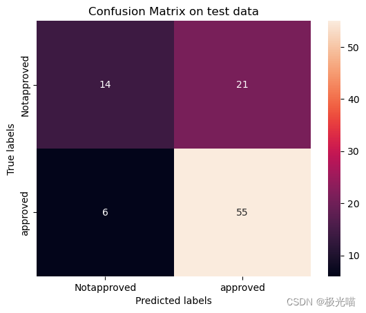
Confusion matrix on trained and test data
# Get the confusion matrix for trained datalabels = ['Notapproved', 'approved']
cm = confusion_matrix(y_train, train_class_preds)
print(cm)ax= plt.subplot()
sns.heatmap(cm, annot=True, ax = ax) #annot=True to annotate cells# labels, title and ticks
ax.set_xlabel('Predicted labels')
ax.set_ylabel('True labels')
ax.set_title('Confusion Matrix on trained data')
ax.xaxis.set_ticklabels(labels)
ax.yaxis.set_ticklabels(labels)
plt.show()# Get the confusion matrix for test datalabels = ['Notapproved', 'approved']
cm = confusion_matrix(y_test, test_class_preds)
print(cm)ax= plt.subplot()
sns.heatmap(cm, annot=True, ax = ax); #annot=True to annotate cells# labels, title and ticks
ax.set_xlabel('Predicted labels')
ax.set_ylabel('True labels')
ax.set_title('Confusion Matrix on test data')
ax.xaxis.set_ticklabels(labels)
ax.yaxis.set_ticklabels(labels)
[[ 61 52][ 7 264]]

[[14 21][ 6 55]]
[Text(0, 0.5, 'Notapproved'), Text(0, 1.5, 'approved')]
随机森林
# applying Random forrest classifier with Hyperparameter tuning
from sklearn.ensemble import RandomForestClassifier
rf = RandomForestClassifier()
grid_values = {'n_estimators':[50, 80,  100], 'max_depth':[4,5,6,7,8,9,10]}
rf_gd = GridSearchCV(rf, param_grid = grid_values, scoring = 'roc_auc', cv=5)# Fit the object to train dataset
rf_gd.fit(X_train, y_train)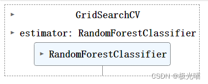
train_class_preds = rf_gd.predict(X_train)
test_class_preds = rf_gd.predict(X_test)
Accuracy Score
# Get the accuracy scores
train_accuracy = accuracy_score(train_class_preds,y_train)
test_accuracy = accuracy_score(test_class_preds,y_test)print("The accuracy on train data is ", train_accuracy)
print("The accuracy on test data is ", test_accuracy)
The accuracy on train data is 0.890625 The accuracy on test data is 0.75
roc_auc Score
# Get the roc_auc scores
train_roc_auc = accuracy_score(y_train,train_class_preds)
test_roc_auc = accuracy_score(y_test,test_class_preds)print("The accuracy on train data is ", train_roc_auc)
print("The accuracy on test data is ", test_roc_auc)
The accuracy on train data is 0.890625 The accuracy on test data is 0.75
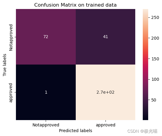
Confusion Matrix
# Get the confusion matrix for trained datalabels = ['Notapproved', 'approved']
cm = confusion_matrix(y_train, train_class_preds)
print(cm)ax= plt.subplot()
sns.heatmap(cm, annot=True, ax = ax) #annot=True to annotate cells# labels, title and ticks
ax.set_xlabel('Predicted labels')
ax.set_ylabel('True labels')
ax.set_title('Confusion Matrix on trained data')
ax.xaxis.set_ticklabels(labels)
ax.yaxis.set_ticklabels(labels)
plt.show()# Get the confusion matrix for test datalabels = ['Notapproved', 'approved']
cm = confusion_matrix(y_test, test_class_preds)
print(cm)ax= plt.subplot()
sns.heatmap(cm, annot=True, ax = ax); #annot=True to annotate cells# labels, title and ticks
ax.set_xlabel('Predicted labels')
ax.set_ylabel('True labels')
ax.set_title('Confusion Matrix on test data')
ax.xaxis.set_ticklabels(labels)
ax.yaxis.set_ticklabels(labels)
plt.show()
[[ 72 41][ 1 270]]
[[13 22][ 2 59]]
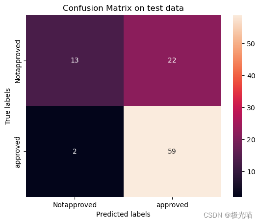
- 最佳 roc_auc 分数源于随机森林分类器,因此随机森林是该模型的最佳预测模型。
代码与数据集下载
详情请见金融贷款批准预测项目-VenusAI (aideeplearning.cn)
相关文章:
金融贷款批准预测项目
注意:本文引用自专业人工智能社区Venus AI 更多AI知识请参考原站 ([www.aideeplearning.cn]) 在金融服务行业,贷款审批是一项关键任务,它不仅关系到资金的安全,还直接影响到金融机构的运营效率和风险管理…...

FR中隐藏系统管理--用户管理中 表格中每条数据中的编辑按钮,删除按钮
比如隐藏删除按钮: var userTableTools BI.Constants.getConstant("dec.constant.user.table.tools")for(var key in userTableTools){if(key "delete"){var deleteItem userTableTools["delete"]deleteItem.invisible true;}}...

函数重载和引用【C++】
文章目录 函数重载什么是函数重载?函数重载的作用使用函数重载的注意点为什么C可以函数重载,C语言不行? 引用什么是引用?引用的语法引用的特点引用的使用场景引用的底层实现传参时传引用和传值的效率引用和指针的区别 函数重载 什…...

rust-tokio发布考古
源头: Carl Lerche Aug 4, 2016 I’m very excited to announce a project that has been a long time in the making. 我很兴奋地宣布一个酝酿已久的项目。 Tokio is a network application framework for rapid development and highly scalable deployments…...
3D医疗图像配准 | 基于Vision-Transformer+Pytorch实现的3D医疗图像配准算法
项目应用场景 面向医疗图像配准场景,项目采用 Pytorch ViT 来实现,形态为 3D 医疗图像的配准。 项目效果 项目细节 > 具体参见项目 README.md (1) 模型架构 (2) Vision Transformer 架构 (3) 量化结果分析 项目获取 https://download.csdn.net/down…...
:状态模式)
设计模式(18):状态模式
核心 用于解决系统中复杂对象的状态转换以及不同状态下行为的封装问题 结构 环境类(Context): 环境类中维护一个State对象,它定义了当前的状态,并委托当前状态处理一些请求; 抽象状态类(State): 用于封装对象的一个特定状态所对应的行为&a…...

如果用大模型考公,kimi、通义千问谁能考高分?
都说大模型要超越人类了,今天就试试让kimi和通义千问做公务员考试题目,谁能考高分? 测评结果再次让人震惊! 问题提干:大小两种规格的盒装鸡蛋,大盒装23个,小盒装16个,采购员小王买了…...

如何在Java中创建对象输入流
在Java中创建对象输入流(ObjectInputStream)通常涉及以下步骤: 获取源输入流:首先,你需要有一个源输入流,它可能来自文件、网络连接或其他任何可以提供字节序列的源。 包装源输入流:接着&#…...

Vue 打包或运行时报错Error: error:0308010C
问题描述: 报错:Error: error:0308010C 报错原因: 主要是因为 nodeJs V17 版本发布了 OpenSSL3.0 对算法和秘钥大小增加了更为严格的限制,nodeJs v17 之前版本没影响,但 V17 和之后版本会出现这个错误…...

222222222222222222222222
欢迎关注博主 Mindtechnist 或加入【Linux C/C/Python社区】一起学习和分享Linux、C、C、Python、Matlab,机器人运动控制、多机器人协作,智能优化算法,滤波估计、多传感器信息融合,机器学习,人工智能等相关领域的知识和…...

微信小程序 电影院售票选座票务系统5w7l6
uni-app框架:使用Vue.js开发跨平台应用的前端框架,编写一套代码,可编译到Android、小程序等平台。 框架支持:springboot/Ssm/thinkphp/django/flask/express均支持 前端开发:vue.js 可选语言:pythonjavanode.jsphp均支持 运行软件…...
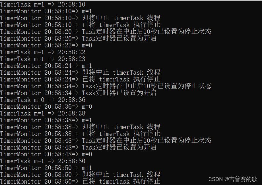
C#:用定时器监控定时器,实现中止定时器正在执行的任务,并重启
Windows服务中使用的比较多的是定时器,但这种定时任务有个比较大的毛病:有时会莫名其妙地停止执行(长时间执行不完,假死),必须得手工重启Windows服务才能恢复正常。这个就太麻烦了。 有没有办法来实现定时…...
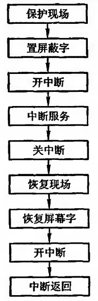
计算机组成原理 — CPU 的结构和功能
CPU 的结构和功能 CPU 的结构和功能CPU 概述控制器概述CPU 框架图CPU 寄存器控制单元 CU 指令周期概述指令周期的数据流 指令流水概述指令流水的原理影响流水线性能的因素流水线的性能流水线的多发技术流水线结构 中断系统概述中断请求标记和中断判优逻辑中断请求标记 INTR中断…...

npm包安装与管理:深入解析命令行工具的全方位操作指南,涵盖脚本执行与包发布流程
npm,全称为Node Package Manager,是专为JavaScript生态系统设计的软件包管理系统,尤其与Node.js平台紧密关联。作为Node.js的默认包管理工具,npm为开发者提供了便捷的方式来安装、共享、分发和管理代码模块。 npm作为JavaScript世…...
实现一个TCP服务器(C++))
序列化结构(protobuf)实现一个TCP服务器(C++)
Protocol Buffers(protobuf)是一种由Google开发的用于序列化结构化数据的方法,通常用于在不同应用程序之间进行数据交换或存储数据。它是一种语言无关、平台无关、可扩展的机制,可以用于各种编程语言和环境中。 1、首先建立proto文…...

Python中的list()和map() 用法
list() 在Python中,list() 是一个内置函数,用于创建列表(list)对象。它有几个不同的用途,但最常见的是将一个可迭代对象(如元组、字符串、集合或其他列表)转换为一个新的列表。 以下是一些使用…...

公网环境下如何端口映射?
公网端口映射是一种网络技术,它允许将本地网络中的设备暴露在公共互联网上,以便能够从任何地方访问这些设备。通过公网端口映射,用户可以通过互联网直接访问和控制局域网中的设备,而无需在本地网络中进行复杂的配置。 公网端口映射…...

7-36 输入年份和月份
输入一个年份和月份,输出这个月的天数。 输入格式: 输入年份year和月份month,年份和月份中间用一个空格隔开。 输出格式: 输入year年的month月对应的天数。 输入样例: 2000 2输出样例: 29输入样例: 1900 2输出样例: 28输入样例: 1900 6输出样例…...

Linux C++ 023-类模板
Linux C 023-类模板 本节关键字:Linux、C、类模板 相关库函数:getCapacity、getSize 类模板语法 类模板的作用:建立一个通用的类,类中的成员 数据类型可以不具体制定, 用一个虚拟的类型代表语法: templa…...
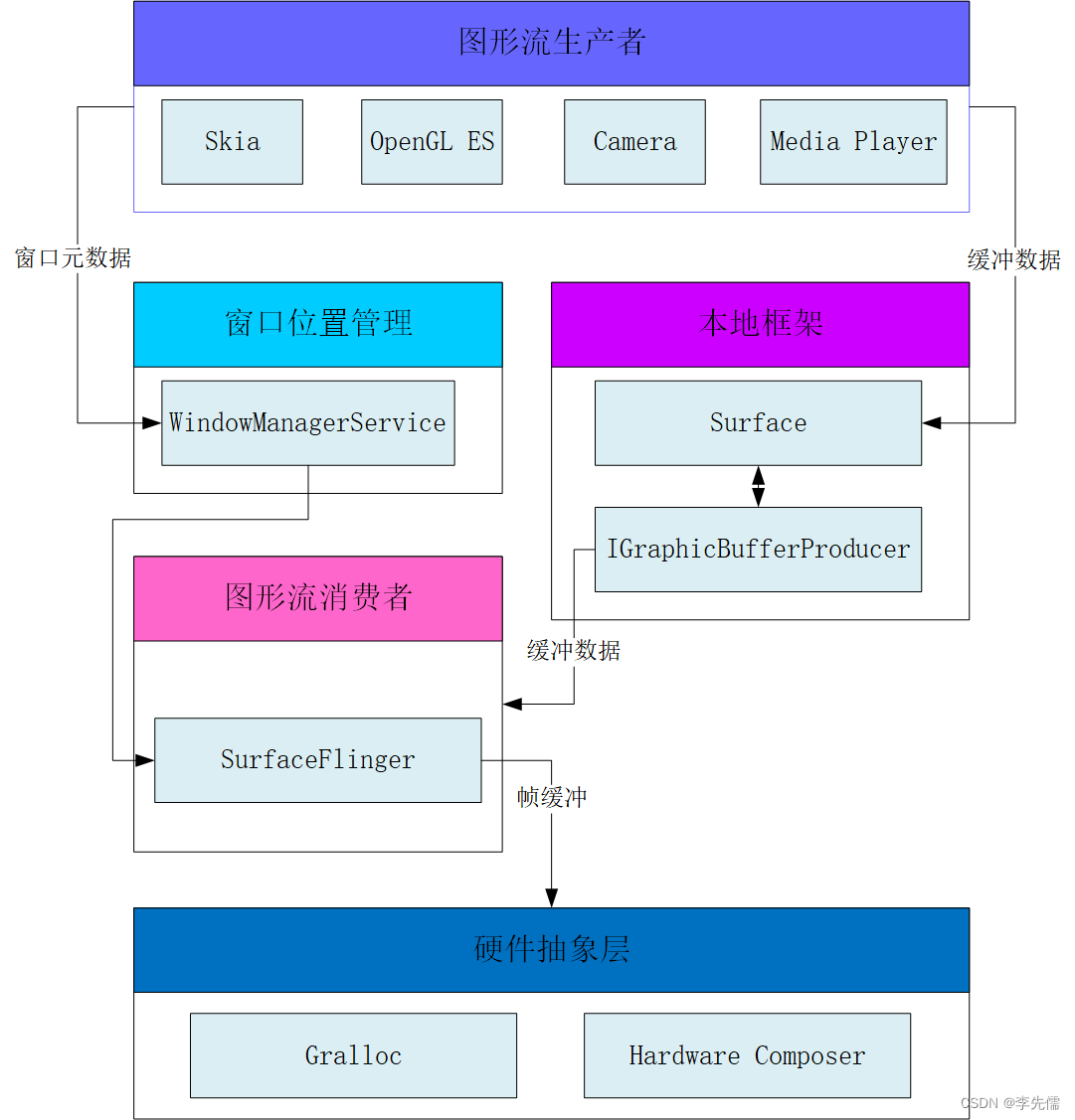
Android图形显示架构概览
图形显示系统作为Android系统核心的子系统,掌握它对于理解Android系统很有帮助,下面从整体上简单介绍图形显示系统的架构,如下图所示。 这个框架只包含了用户空间的图形组件,不涉及底层的显示驱动。框架主要包括以下4个图形组件。…...
)
告别卡顿!用GDAL+ObjectARX在AutoCAD里丝滑加载百GB遥感影像(附C++源码)
告别卡顿!用GDALObjectARX在AutoCAD里丝滑加载百GB遥感影像(附C源码) 在GIS和测绘工程领域,处理海量遥感影像数据是家常便饭。但当这些GB级甚至TB级的航拍图、卫星图需要导入AutoCAD进行规划设计时,传统的RasterImage对…...

8051嵌入式开发中的数据覆盖与代码分页技术详解
1. A51汇编中的数据覆盖与代码分页技术解析在8051嵌入式开发中,内存资源往往捉襟见肘。我曾在一个烟雾报警器项目中,主控芯片只有128字节RAM和4KB Flash,却要实现复杂的烟雾浓度算法和无线通信协议。正是通过数据覆盖(Data Overlaying)和代码…...

微信读书笔记助手:3分钟快速上手的终极笔记管理指南
微信读书笔记助手:3分钟快速上手的终极笔记管理指南 【免费下载链接】wereader 一个浏览器扩展:主要用于微信读书做笔记,对常使用 Markdown 做笔记的读者比较有帮助。 项目地址: https://gitcode.com/gh_mirrors/wer/wereader 微信读书…...

从电机控制到服务器电源:详解功率MOSFET栅极外加电容CGS与CGD的选型计算与布局要点
功率MOSFET栅极电容设计实战:从电机驱动到服务器电源的差异化策略 在电力电子系统的核心地带,功率MOSFET如同精密交响乐团的指挥,其开关性能直接决定整个系统的效率与可靠性。当我们面对电机驱动系统要求快速切换以降低损耗,或是服…...

AMD Ryzen处理器底层调试技术解析:SMUDebugTool的架构设计与实践应用
AMD Ryzen处理器底层调试技术解析:SMUDebugTool的架构设计与实践应用 【免费下载链接】SMUDebugTool A dedicated tool to help write/read various parameters of Ryzen-based systems, such as manual overclock, SMU, PCI, CPUID, MSR and Power Table. 项目地…...

DLSS Swapper终极指南:一键管理游戏图形增强文件,释放显卡全部性能
DLSS Swapper终极指南:一键管理游戏图形增强文件,释放显卡全部性能 【免费下载链接】dlss-swapper 项目地址: https://gitcode.com/GitHub_Trending/dl/dlss-swapper DLSS Swapper是一款专为游戏玩家设计的智能图形增强文件管理工具,…...

如何解决Noah-MP陆面模型编译与配置中的三大技术挑战
如何解决Noah-MP陆面模型编译与配置中的三大技术挑战 【免费下载链接】NoahMP 项目地址: https://gitcode.com/gh_mirrors/no/NoahMP Noah-MP(Noah with Multi-Parameterization options)作为先进的陆面过程模型,在水文循环模拟、能量…...

【NotebookLM图书馆学研究实战指南】:20年图情专家亲授AI时代知识管理新范式
更多请点击: https://codechina.net 第一章:NotebookLM图书馆学研究的范式革命 传统图书馆学研究长期依赖人工文献综述、卡片目录索引与线性知识组织方式,而NotebookLM的引入正从根本上重构知识发现、关联与推理的底层逻辑。作为Google推出的…...

Arm DynamIQ™ DSU架构解析与多核设计优化
1. Arm DynamIQ™ Shared Unit架构深度解析 在当代SoC设计中,多核处理器架构面临的核心挑战是如何在提升计算密度的同时,维持高效的数据一致性与灵活的功耗管理。Arm DynamIQ™ Shared Unit(DSU)作为解决这一问题的创新设计&#…...

APK Installer终极指南:Windows平台Android应用部署完全手册
APK Installer终极指南:Windows平台Android应用部署完全手册 【免费下载链接】APK-Installer An Android Application Installer for Windows 项目地址: https://gitcode.com/GitHub_Trending/ap/APK-Installer 在跨平台应用生态日益融合的今天,开…...