vst 算法R语言手工实现 | Seurat4 筛选高变基因的算法
1. vst算法描述
(1)为什么需要矫正

image source: https://ouyanglab.com/singlecell/basic.html
In this panel, we observe that there is a very strong positive relationship between a gene’s average expression and its observed variance. In other words, highly expressed genes have high variances associated with them and vice versa. This phenomenon is often referred to as heteroskedasticity within the data and must be corrected before proceeding with any downstream analysis steps.
高表达的基因其变异也高。这被叫做数据内的 异方差性,必须矫正后才能进一步下游分析。
In short, the dependance of a gene’s expression with its observed variance is what needs to be corrected prior to HVG selection [1].
简而言之,基因表达与其观察到的变异的依赖性是在HVG选择之前需要纠正的。
The Solution:
A very common way to correct this problem is by applying a Variance Stabilizing Transformation (VST) to the data, and we see in the right panel of the above figure that once VST is applied, the relationship of observed variance at any given level of average expression for a gene has been removed/standardized.
(2)Seurat4 R文档
> ?FindVariableFeatures
vst:
- First, fits a line to the relationship of log(variance) and log(mean) using local polynomial regression (loess).
- Then standardizes the feature values using the observed mean and expected variance (given by the fitted line).
- Feature variance is then calculated on the standardized values after clipping to a maximum (see clip.max parameter).
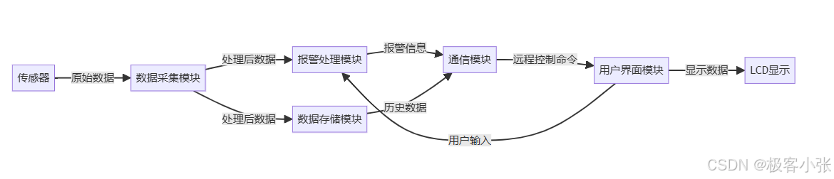
vst steps: 目的是在var~mean曲线中,不同mean值区域都能挑选var较大的基因
- 使用局部多项式拟合(loess) log(variance) 和log(mean) 平滑曲线模型
- 获取模型计算的值作为y=var.exp值
- 截取最大之后,var.standarlized = get variance after feature standardization:
(每个基因 - mean)/sd 后 取var(). 注意sd=sqrt(var.exp) - 按照 var.standarlized 降序排列,取前n(比如2000)个基因作为高变基因。
2. 加载数据及Seurat vst 结果
使用pbmc 3k数据,走标准Seurat4,选取top 2000 HVG [2]。
library(Seurat)
library(ggplot2)
library(dplyr)pbmc=readRDS("d:\\code_R\\filtered_gene_bc_matrices\\pbmc3k.final.Rds")
DimPlot(pbmc, label=T)# pbmc <- FindVariableFeatures(pbmc, selection.method = "vst", nfeatures = 2000)# 0. 获取Seurat包计算的HVG ----
top10 <- head(VariableFeatures(pbmc), 10)
p1=VariableFeaturePlot(pbmc); p1
LabelPoints(plot = p1, points = top10, repel = TRUE)genelist1=VariableFeatures(pbmc)
length(genelist1)
head(genelist1)head( pbmc@assays$RNA@meta.features )
3. 手工 HVG
(1) LOESS fit y~x
log(variance) ~ log(mean)
# use raw data: vst 的直接输入的是 counts,所以直接算的 行平均数,作为基因表达值
counts = pbmc@assays$RNA@counts# 计算每行均值
hvf.info <- data.frame(mean = rowMeans(x = counts, na.rm = T))# 计算每行方差
hvf.info$variance = apply(counts, 1, function(x){var(x, na.rm = T)
})head(hvf.info)
dim(hvf.info)if(0){#pdf( paste0(outputRoot, keyword, "_01_4B.HVG.pdf"), width=5.5, height =4.8)plot(hvf.info$mean, hvf.info$variance, pch=19, cex=0.3)plot(log10(hvf.info$mean), hvf.info$variance, pch=19, cex=0.3)plot(log10(hvf.info$mean), log10(hvf.info$variance), pch=19, cex=0.3) #looks good#dev.off()
}# 通过loess拟合,计算期望方差和标准化的方差
hvf.info$variance.expected <- 0
hvf.info$variance.standardized <- 0not.const <- (hvf.info$variance >0) & (!is.na(hvf.info$variance)) & (!is.na(hvf.info$mean))
table(not.const)
#TRUE
#13714# 拟合 y~x
loess.span=0.3 #default in Seurat4
fit <- loess(formula = log10(x = variance) ~ log10(x = mean),data = hvf.info[not.const, ],span = loess.span
)dim(hvf.info[not.const, ]) #13714     4
#str(fit)
(2). 获取模型给出的期望y值
# 期望y值:使用模型计算的值
hvf.info$variance.expected[not.const] <- 10 ^ fit$fitted
(3). 截取极端值后,计算标准化后的方差
#clip.max == 'auto',则自动设置为 列数(细胞数)的开方
clip.max <- sqrt(x = ncol(x = counts))
clip.max #51.9# 计算feature标准化( (counts - mean)/sd )后的方差,注意sd=sqrt(var)
# 求方差前截取极大值
hvf.info$variance.standardized[not.const]=(function(){result=c()for(i in 1:nrow(counts)){row.var=NAif(not.const[i]){# clip to a maximumrow.counts.std = (counts[i, ] - hvf.info$mean[i]) / sqrt(hvf.info$variance.expected[i])row.counts.std[row.counts.std>clip.max]=clip.max# 计算方差row.var=var( row.counts.std, na.rm = T )}# 返回结果result=c(result, row.var)}return(result)
})() #2min
(4) 第(3)步主要参考
来源是Seurat4 函数FindVariableFeatures.default 中:
hvf.info$variance.standardized <- SparseRowVarStd(mat = object,mu = hvf.info$mean,sd = sqrt(hvf.info$variance.expected),vmax = clip.max,display_progress = verbose)
查找SparseRowVarStd的定义:
$ find .| xargs grep -in "SparseRowVarStd" --color=auto
grep: .: Is a directory
./data_manipulation.cpp:305:NumericVector SparseRowVarStd(Eigen::SparseMatrix<double> mat,
./data_manipulation.h:40:NumericVector SparseRowVarStd(Eigen::SparseMatrix<double> mat,
./RcppExports.cpp:185:// SparseRowVarStd
./RcppExports.cpp:186:NumericVector SparseRowVarStd(Eigen::SparseMatrix<double> mat, NumericVector mu, NumericVector sd, double vmax, bool display_progress);
./RcppExports.cpp:187:RcppExport SEXP _Seurat_SparseRowVarStd(SEXP matSEXP, SEXP muSEXP, SEXP sdSEXP, SEXP vmaxSEXP, SEXP display_progressSEXP) {
./RcppExports.cpp:195:    rcpp_result_gen = Rcpp::wrap(SparseRowVarStd(mat, mu, sd, vmax, display_progress));
./RcppExports.cpp:421:    {"_Seurat_SparseRowVarStd", (DL_FUNC) &_Seurat_SparseRowVarStd, 5},
发现是Seurat4 的 c++函数,定义在 seurat-4.1.0/src/data_manipulation.cpp:301
/* standardize matrix rows using given mean and standard deviation,clip values larger than vmax to vmax,then return variance for each row */
// [[Rcpp::export(rng = false)]]
NumericVector SparseRowVarStd(Eigen::SparseMatrix<double> mat,NumericVector mu,NumericVector sd,double vmax,bool display_progress){if(display_progress == true){Rcpp::Rcerr << "Calculating feature variances of standardized and clipped values" << std::endl;}mat = mat.transpose();NumericVector allVars(mat.cols());Progress p(mat.outerSize(), display_progress);for (int k=0; k<mat.outerSize(); ++k){p.increment();if (sd[k] == 0) continue;double colSum = 0;int nZero = mat.rows();for (Eigen::SparseMatrix<double>::InnerIterator it(mat,k); it; ++it){nZero -= 1;colSum += pow(std::min(vmax, (it.value() - mu[k]) / sd[k]), 2);}colSum += pow((0 - mu[k]) / sd[k], 2) * nZero;allVars[k] = colSum / (mat.rows() - 1);}return(allVars);
}
结合R的上下文,大致能猜出来c++代码啥意思。
想看懂细节,则需要更多c++知识储备:
- cpp最顶部的头文件:
#include <RcppEigen.h>
#include <progress.hpp>
#include <cmath>
#include <unordered_map>
#include <fstream>
#include <string>
#include <Rinternals.h>using namespace Rcpp;
Eigen::SparseMatrix<double> mat:泛型;矩阵::系数矩阵- 稀疏矩阵的方法:
mat.transpose(),mat.cols(),mat.outerSize(), for (Eigen::SparseMatrix<double>::InnerIterator it(mat,k); it; ++it): 集合的迭代器- Rcpp 数据类型:
NumericVector,
4. 结果比较
(1) 结果检查1:基因列表一致
手工计算的和Seurat4的HVG gene list结果完全一致。
# Check 1: HVG gene list
hvf.info=hvf.info[order(-hvf.info$variance.standardized),]
head(hvf.info)
tail(hvf.info)
#top.features=head( rownames(hvf.info), n=250)
top.features_2=head( rownames(hvf.info), n=2000)
length(top.features_2)
head(top.features_2)
setdiff(top.features_2, genelist1)
setdiff(genelist1, top.features_2)
#
if(0){# Check: gene and their parampbmc@assays$RNA@meta.features[c(setdiff(genelist1, top.features_2)),]hvf.info[c(setdiff(genelist1, top.features_2)),]#pbmc@assays$RNA@meta.features[c(setdiff(top.features_2, genelist1)),]hvf.info[c(setdiff(top.features_2, genelist1)),]
}
(2) 结果检查2:基因参数一致
手工计算的和Seurat4的HVG gene 参数完全一致。
# check2: HVG and its params
# 1.
dim(pbmc@assays$RNA@meta.features)
head( pbmc@assays$RNA@meta.features )
#                 vst.mean vst.variance vst.variance.expected vst.variance.standardized vst.variable
#AL627309.1    0.003333333  0.003323453           0.003575582                 0.9294859        FALSE
#AP006222.2    0.001111111  0.001110288           0.001112798                 0.9977442        FALSE
#RP11-206L10.2 0.001851852  0.001849107           0.001921811                 0.9621691        FALSE
#RP11-206L10.9 0.001111111  0.001110288           0.001112798                 0.9977442        FALSE
#LINC00115     0.006666667  0.006624676           0.007342308                 0.9022607        FALSE
#NOC2L         0.106666667  0.158310485           0.203482316                 0.7780061        FALSE# 2.
dim(hvf.info)
hvf.info=hvf.info[rownames(pbmc@assays$RNA@meta.features),]
head(hvf.info)
#                     mean    variance variance.expected variance.standardized
#AL627309.1    0.003333333 0.003323453       0.003575582             0.9294859
#AP006222.2    0.001111111 0.001110288       0.001112798             0.9977442
#RP11-206L10.2 0.001851852 0.001849107       0.001921811             0.9621691
#RP11-206L10.9 0.001111111 0.001110288       0.001112798             0.9977442
#LINC00115     0.006666667 0.006624676       0.007342308             0.9022607
#NOC2L         0.106666667 0.158310485       0.203482316             0.7780061
比较高变基因的参数:
> hvf.info[genelist1|> head(), ]mean    variance variance.expected variance.standardized
PPBP    0.2451852    9.577506         0.5888573             11.171153
S100A9  6.0466667  278.681037        34.8969051              7.985838
IGLL5   0.2792593    8.894938         0.6929479              7.964379
LYZ    10.2466667  564.108825        70.8492711              7.962098
GNLY    1.5740741   45.239046         6.0378423              7.492585
FTL    27.6674074 2008.688897       278.9968379              7.199683
> pbmc@assays$RNA@meta.features[genelist1|> head(), ]vst.mean vst.variance vst.variance.expected vst.variance.standardized vst.variable
PPBP    0.2451852     9.577506             0.5888573                 11.172765         TRUE
S100A9  6.0466667   278.681037            34.8969051                  7.985838         TRUE
IGLL5   0.2792593     8.894938             0.6929479                  7.965360         TRUE
LYZ    10.2466667   564.108825            70.8492711                  7.962098         TRUE
GNLY    1.5740741    45.239046             6.0378423                  7.492585         TRUE
FTL    27.6674074  2008.688897           278.9968379                  7.199683         TRUE> table(abs(hvf.info[genelist1, 4] - pbmc@assays$RNA@meta.features[genelist1, 4])<0.005)
FALSE  TRUE 3  1997# 差别不大,差异的绝对值大于0.005的共三个:
> keep2=abs(hvf.info[genelist1, 4] - pbmc@assays$RNA@meta.features[genelist1, 4])>0.005
> table(keep2)
keep2
FALSE  TRUE 1997     3 > hvf.info[genelist1, ][keep2, ]mean  variance variance.expected variance.standardized
IGJ      0.16777778 16.822896        0.36540081              3.481455
SLC48A1  0.03370370  0.871409        0.04618194              2.215032
NAPA-AS1 0.02962963  1.050622        0.03932270              1.274513
> pbmc@assays$RNA@meta.features[genelist1, ][keep2, ]vst.mean vst.variance vst.variance.expected vst.variance.standardized vst.variable
IGJ      0.16777778    16.822896            0.36540081                  3.498952         TRUE
SLC48A1  0.03370370     0.871409            0.04618194                  2.220942         TRUE
NAPA-AS1 0.02962963     1.050622            0.03932270                  1.280866         TRUE
最后一列略有区别:
#
all( abs(hvf.info[,1] - pbmc@assays$RNA@meta.features[,1]) < 1e-6) #T
all( abs(hvf.info[,2] - pbmc@assays$RNA@meta.features[,2]) < 1e-6) #T
all( abs(hvf.info[,3] - pbmc@assays$RNA@meta.features[,3]) < 1e-6) #Ttable( abs(hvf.info[,4] - pbmc@assays$RNA@meta.features[,4]) < 1e-6) #not all T
table( abs(hvf.info[,4] - pbmc@assays$RNA@meta.features[,4]) < 0.01)
#FALSE  TRUE
#    1 13713keep = abs(hvf.info[,4] - pbmc@assays$RNA@meta.features[,4]) > 1e-2> table(keep)
keep
FALSE  TRUE
13713     1
> hvf.info[keep, ]mean variance variance.expected variance.standardized
IGJ 0.1677778  16.8229         0.3654008              3.481455
> pbmc@assays$RNA@meta.features[keep, ]vst.mean vst.variance vst.variance.expected vst.variance.standardized vst.variable
IGJ 0.1677778      16.8229             0.3654008                  3.498952         TRUE
(3) 绘图比较
 (a) var~avg with top 2000 HVG selected by vst;
(b) std.var ~ avg with top 2000 HVG selected by vst;
( c) same as (b), but draw by Seurat functions.
# plot1
plot(log10(hvf.info$mean), log10(hvf.info$variance), pch=19, cex=0.3, main="vst manully #1", mgp=c(2,1,0))
points(log10(hvf.info[top.features_2, ]$mean), log10(hvf.info[top.features_2, ]$variance), pch=19, cex=0.3, col="red")# plot2
plot(log10(hvf.info$mean), hvf.info$variance.standardized, pch=19, cex=0.3, main="vst manully #2", mgp=c(2,1,0))
points(log10(hvf.info[top.features_2,]$mean), (hvf.info[top.features_2,]$variance.standardized), pch=19, cex=0.3, col="red")# plot3: Seurat
LabelPoints(plot = p1, points = top10, repel = TRUE)
#
Ref:
- [1] https://medium.com/byte-sized-machine-learning/selection-of-highly-variable-genes-hvgs-in-scrna-seq-647c8eee3845
- [2] https://zhuanlan.zhihu.com/p/479549742
相关文章:
vst 算法R语言手工实现 | Seurat4 筛选高变基因的算法
1. vst算法描述 (1)为什么需要矫正 image source: https://ouyanglab.com/singlecell/basic.html In this panel, we observe that there is a very strong positive relationship between a gene’s average expression and its observed variance. I…...

阿里通义千问大模型Qwen2-72B-Instruct通用能力登顶国内第一!
前言: 中国互联网协会副秘书长裴玮近日在2024中国互联网大会上发布《中国互联网发展报告(2024)》。《报告》指出, 在人工智能领域,2023年我国人工智能产业应用进程持续推进,核心产业规模达到5784亿元。 截至2024年3月ÿ…...

CH04_依赖项属性
第4章:依赖项属性 本章目标 理解依赖项属性理解属性验证 依赖项属性 属性与事件是.NET抽象模型的核心部分。WPF使用了更高级的依赖项属性(Dependency Property)功能来替换原来.NET的属性,实现了更高效率的保存机制…...

CentOS 7开启SSH连接
1. 安装openssh-server 1.1 检查是否安装openssh-server服务 yum list installed | grep openssh-server如果有显示内容,则已安装跳过安装步骤,否则进行第2步 1.2 安装openssh-server yum install openssh-server2. 开启SSH 22监听端口 2.1 打开ssh…...

代理伺服器分類詳解
代理伺服器的主要分類 代理伺服器可以根據不同的標準進行分類。以下是幾種常見的分類方式: 按協議分類按匿名性分類按使用場景分類 1. 按協議分類 根據支持的協議類型,代理伺服器可以分為以下幾類: HTTP代理:專門用於處理HTT…...

计数,桶与基数排序
目录 一. 计数排序 概念 步骤思路如下 实现代码如下 时间复杂度与空间复杂度 1. 时间复杂度 2. 空间复杂度 计数排序的特点 二. 桶排序 概念 步骤思路如下 实现代码如下 时间复杂度与空间复杂度 1. 时间复杂度 2. 空间复杂度 桶排序的特点 三. 基数排序 概念 步…...

unity渲染人物模型透明度问题
问题1:有独立的手和衣服的模型,但最终只渲染出来半透明衣服 问题2:透明度贴图是正确的但显示却不正确 这上面两个模型的问题都是因为人物模型是一个完整的,为啥有些地方可以正常显示,有些地方透明度却有问题。 其中…...

CH03_布局
第3章:布局 本章目标 理解布局的原则理解布局的过程理解布局的容器掌握各类布局容器的运用 理解 WPF 中的布局 WPF 布局原则 WPF 窗口只能包含单个元素。为在WPF 窗口中放置多个元素并创建更贴近实用的用户男面,需要在窗口上放置一个容器&#x…...

【Oracle】Oracle中的merge into
目录 解释使用场景语法示例案例一案例二 MERGE INTO的优缺点优点:缺点: 注意事项附:Oracle中的MERGE INTO实现的效果,如果改为用MySQL应该怎么实现注意 解释 在Oracle数据库中,MERGE INTO是一种用于对表进行合并&…...
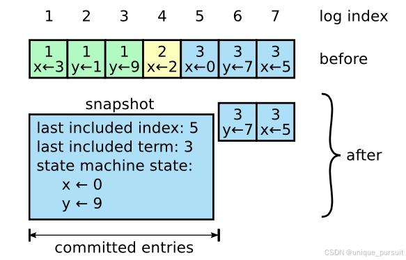
【论文阅读笔记】In Search of an Understandable Consensus Algorithm (Extended Version)
1 介绍 分布式一致性共识算法指的是在分布式系统中,使得所有节点对同一份数据的认知能够达成共识的算法。且算法允许所有节点像一个整体一样工作,即使其中一些节点出现故障也能够继续工作。之前的大部分一致性算法实现都是基于Paxos,但Paxos…...
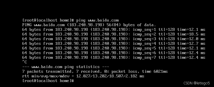
CentOS 7 网络配置
如想了解请查看 虚拟机安装CentOS7 第一步:查看虚拟机网络编辑器、查看NAT设置 (子网ID,网关IP) 第二步:配置VMnet8 IP与DNS 注意事项:子网掩码与默认网关与 第一步 保持一致 第三步:网络配置…...

2024 React 和 Vue 的生态工具
react Vue...

AI学习指南机器学习篇-t-SNE模型应用与Python实践
AI学习指南机器学习篇-t-SNE模型应用与Python实践 在机器学习领域,数据的可视化是非常重要的,因为它可以帮助我们更好地理解数据的结构和特征。而t-SNE(t-distributed Stochastic Neighbor Embedding)是一种非常强大的降维和可视…...

小试牛刀-Telebot区块链游戏机器人
目录 1.编写目的 2.实现功能 2.1 Wallet功能 2.2 游戏功能 2.3 提出功能 2.4 辅助功能 3.功能实现详解 3.1 wallet功能 3.2 游戏功能 3.3 提出功能 3.4 辅助功能 4.测试视频 Welcome to Code Blocks blog 本篇文章主要介绍了 [Telebot区块链游戏机器人] ❤博主…...
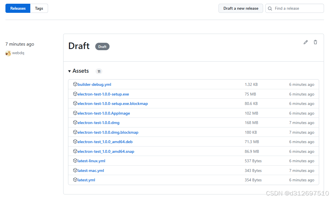
使用github actions构建多平台electron应用
1. 创建electron项目 使用pnpm创建项目 pnpm create quick-start/electron 2. 修改electron-builder.yml文件 修改mac的target mac:target:- target: dmgarch: universal 3. 添加workflow 创建 .github/workflows/main.yml 文件 name: Build/release Electron appon:work…...

java通过pdf-box插件完成对pdf文件中图片/文字的替换
需要引入的Maven依赖: <!-- pdf替换图片 --><dependency><groupId>e-iceblue</groupId><artifactId>spire.pdf.free</artifactId><version>5.1.0</version></dependency> java代码: public AjaxResult replacepd…...
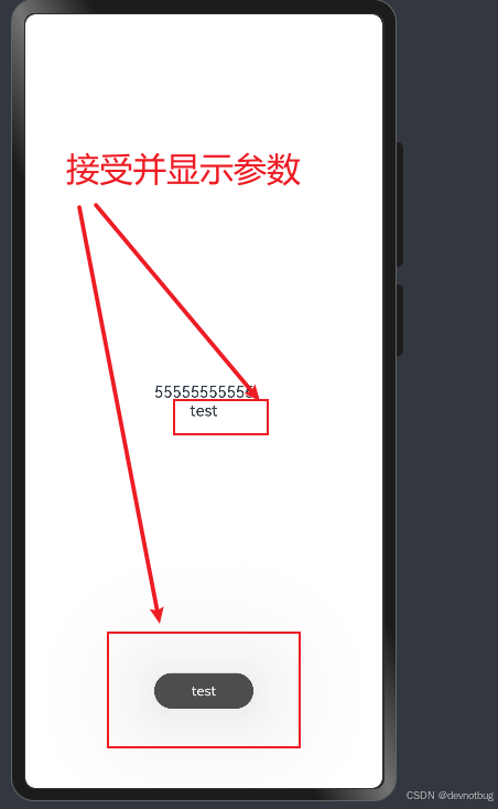
鸿蒙 next 5.0 版本页面跳转传参 接受参数 ,,接受的时候 要先定义接受参数的类型, 代码可以直接CV使用 [教程]
1, 先看效果 2, 先准备好两个页面 index 页面 传递参数 import router from ohos.routerEntry Component struct Index {Statelist: string[] [星期一, 星期二,星期三, 星期四,星期五]StateactiveIndex: number 0build() {Row() {Column({ space: 10 }) {ForEach(this.list,…...

【electron6】浏览器实时播放PCM数据
pcm介绍:PCM(Puls Code Modulation)全称脉码调制录音,PCM录音就是将声音的模拟信号表示成0,1标识的数字信号,未经任何编码和压缩处理,所以可以认为PCM是未经压缩的音频原始格式。PCM格式文件中不包含头部信…...
嵌入式C/C++、FreeRTOS、STM32F407VGT6和TCP:智能家居安防系统的全流程介绍(代码示例)
1. 项目概述 随着物联网技术的快速发展,智能家居安防系统越来越受到人们的重视。本文介绍了一种基于STM32单片机的嵌入式安防中控系统的设计与实现方案。该系统集成了多种传感器,实现了实时监控、报警和远程控制等功能,为用户提供了一个安全、可靠的家居安防解决方案。 1.1 系…...
【Django】django自带后台管理系统样式错乱,uwsgi启动css格式消失的问题
正常情况: ERROR:(css、js文件加载失败) 问题:CSS加载的样式没有了,原因:使用了django自带的admin,在使用 python manage.py runserver启动 的时候,可以加载到admin的文…...

移动端数据抓取实战:基于Capacitor插件实现自动化采集
1. 项目概述:一个为移动端设计的“数据抓手”最近在做一个移动端的数据采集项目,需要从一些应用里提取特定的信息。直接写原生代码去解析页面结构,不仅开发周期长,而且一旦目标应用的界面更新,我们的代码就得跟着改&am…...

API淘宝关键词搜索:运用场所、使用方式及获客逻辑
在电商生态中,淘宝关键词搜索API是连接第三方系统与平台商品数据的核心桥梁。其核心价值在于通过标准化接口,精准、合规地获取关键词对应的商品、店铺及市场数据,为各类业务提供坚实的数据支撑。相较于传统爬虫,API调用具备合规性…...

Keyviz完全指南:5分钟掌握实时键鼠可视化技巧
Keyviz完全指南:5分钟掌握实时键鼠可视化技巧 【免费下载链接】keyviz Keyviz is a free and open-source tool to visualize your keystrokes ⌨️ and 🖱️ mouse actions in real-time. 项目地址: https://gitcode.com/gh_mirrors/ke/keyviz 你…...

大模型压缩实战:量化、剪枝与知识蒸馏技术解析与应用
1. 项目概述:当大模型遇见“瘦身”革命最近在跟几个做AI应用落地的朋友聊天,大家普遍都在吐槽一个事儿:现在的大语言模型(LLM)能力是强,但动辄几十亿、上百亿的参数规模,部署成本高得吓人&#…...
)
基于开关电容器的级联多电平逆变器,使用布尔PWM控制技术研究(Simulink仿真实现)
💥💥💞💞欢迎来到本博客❤️❤️💥💥 🏆博主优势:🌞🌞🌞博客内容尽量做到思维缜密,逻辑清晰,为了方便读者。 ⛳️座右铭&a…...

荔枝派Zero V3s新手避坑指南:从源码编译到SPI Flash烧录u-boot的完整流程
荔枝派Zero V3s开发实战:从源码编译到SPI Flash烧录的避坑手册 第一次拿到荔枝派Zero V3s开发板时,那种既兴奋又忐忑的心情至今记忆犹新。作为全志V3s芯片的经典开发平台,它凭借64MB DDR2内存、内置WiFi和丰富的外设接口,成为嵌入…...

Arm编译器在嵌入式开发中的优化实践
1. Arm编译器嵌入式开发环境概述在嵌入式系统开发领域,工具链的选择往往决定了最终产品的性能上限。作为Arm架构的"原生"编译器,Arm Compiler for Embedded凭借其深度优化的代码生成能力,在物联网设备、工业控制器等资源受限场景中…...

基于RAG与向量数据库的智能知识库构建实战指南
1. 项目概述:一个开源的深度知识库构建与问答引擎最近在折腾一个挺有意思的开源项目,叫deepwiki-open。简单来说,它就是一个帮你把一堆文档(比如公司内部Wiki、产品手册、技术文档)变成一个能“听懂人话”并“对答如流…...

数字永生:将意识上传云端的技术与伦理极限
——一个软件测试从业者的技术解构与风险分析各位同行,当你看到“数字永生”这四个字时,脑海里浮现的是什么?是马斯克口中2045年即将实现的意识上传,还是《黑镜》里那些被困在虚拟牢笼中的数字灵魂?作为一个每天与需求…...

Taotoken官方价折扣活动对于高频用户的实际成本影响分析
🚀 告别海外账号与网络限制!稳定直连全球优质大模型,限时半价接入中。 👉 点击领取海量免费额度 Taotoken官方价折扣活动对于高频用户的实际成本影响分析 1. 理解Taotoken的计费模式 Taotoken平台采用按Token消耗量计费的模式。…...