【机器学习】Multiple Variable Linear Regression
Multiple Variable Linear Regression
- 1、问题描述
- 1.1 包含样例的X矩阵
- 1.2 参数向量 w, b
- 2、多变量的模型预测
- 2.1 逐元素进行预测
- 2.2 向量点积进行预测
- 3、多变量线性回归模型计算损失
- 4、多变量线性回归模型梯度下降
- 4.1 计算梯度
- 4.2梯度下降
首先,导入所需的库
import copy, math
import numpy as np
import matplotlib.pyplot as plt
plt.style.use('./deeplearning.mplstyle')
np.set_printoptions(precision=2)  # reduced display precision on numpy arrays
1、问题描述
使用房价预测的示例来构建线性回归模型。训练数据集包含三个样本,每个样本有四个特征(面积、卧室数、楼层数和年龄),如下表所示。这里的面积以平方英尺(sqft)为单位。
| Size (sqft) | Number of Bedrooms | Number of floors | Age of Home | Price (1000s dollars) |
|---|---|---|---|---|
| 2104 | 5 | 1 | 45 | 460 |
| 1416 | 3 | 2 | 40 | 232 |
| 852 | 2 | 1 | 35 | 178 |
使用这些值构建线性回归模型,从而可以预测其他房屋的价格。例如,给定一个1200平方英尺、3个卧室、1层楼、40岁的房屋,可以用模型来预测其价格。
根据表格数据创建 X_train 和 y_train 变量。
X_train = np.array([[2104, 5, 1, 45], [1416, 3, 2, 40], [852, 2, 1, 35]])
y_train = np.array([460, 232, 178])
1.1 包含样例的X矩阵
与上面的表格类似,样例被存储在一个 NumPy 矩阵X_train 中。矩阵中的每一行表示一个样例。当有 m m m 个训练样例,每个样例有 n n n 个特征时, X \mathbf{X} X 是一个维度为 ( m m m, n n n) 的矩阵(m 行,n 列)。
X = ( x 0 ( 0 ) x 1 ( 0 ) ⋯ x n − 1 ( 0 ) x 0 ( 1 ) x 1 ( 1 ) ⋯ x n − 1 ( 1 ) ⋯ x 0 ( m − 1 ) x 1 ( m − 1 ) ⋯ x n − 1 ( m − 1 ) ) \mathbf{X} = \begin{pmatrix} x^{(0)}_0 & x^{(0)}_1 & \cdots & x^{(0)}_{n-1} \\ x^{(1)}_0 & x^{(1)}_1 & \cdots & x^{(1)}_{n-1} \\ \cdots \\ x^{(m-1)}_0 & x^{(m-1)}_1 & \cdots & x^{(m-1)}_{n-1} \end{pmatrix} X= x0(0)x0(1)⋯x0(m−1)x1(0)x1(1)x1(m−1)⋯⋯⋯xn−1(0)xn−1(1)xn−1(m−1)
notation:
- x ( i ) \mathbf{x}^{(i)} x(i) 是包含第 i 个样例的向量。 x ( i ) = ( x 0 ( i ) , x 1 ( i ) , ⋯ , x n − 1 ( i ) ) \mathbf{x}^{(i)}= (x^{(i)}_0, x^{(i)}_1, \cdots,x^{(i)}_{n-1}) x(i)=(x0(i),x1(i),⋯,xn−1(i))
- x j ( i ) x^{(i)}_j xj(i) 是第 i 个样例中的第 j 个元素。圆括号中的上标表示样例编号,而下标表示元素编号。
# data is stored in numpy array/matrix
print(f"X Shape: {X_train.shape}, X Type:{type(X_train)})")
print(X_train)
print(f"y Shape: {y_train.shape}, y Type:{type(y_train)})")
print(y_train)
1.2 参数向量 w, b
- w \mathbf{w} w 是具有 n n n 个元素的向量
- 每个元素包含一个特征相关的参数
- i在我们的数据集中, n = 4.
- 将这表示为列向量
w = ( w 0 w 1 ⋯ w n − 1 ) \mathbf{w} = \begin{pmatrix} w_0 \\ w_1 \\ \cdots\\ w_{n-1} \end{pmatrix} w= w0w1⋯wn−1
- b b b 是一个标量参数
为了演示, w \mathbf{w} w 和 b b b 将被加载为一些初始选定的值,这些值接近最优解。 w \mathbf{w} w 是一个一维的 NumPy 向量。
b_init = 785.1811367994083
w_init = np.array([ 0.39133535, 18.75376741, -53.36032453, -26.42131618])
print(f"w_init shape: {w_init.shape}, b_init type: {type(b_init)}")
2、多变量的模型预测
多变量的线性回归模型的预测可以表示为:
f w , b ( x ) = w 0 x 0 + w 1 x 1 + . . . + w n − 1 x n − 1 + b (1) f_{\mathbf{w},b}(\mathbf{x}) = w_0x_0 + w_1x_1 +... + w_{n-1}x_{n-1} + b \tag{1} fw,b(x)=w0x0+w1x1+...+wn−1xn−1+b(1)
或用向量表示:
f w , b ( x ) = w ⋅ x + b (2) f_{\mathbf{w},b}(\mathbf{x}) = \mathbf{w} \cdot \mathbf{x} + b \tag{2} fw,b(x)=w⋅x+b(2)
其中 ⋅ \cdot ⋅ 是向量点积
2.1 逐元素进行预测
之前的预测是将一个特征值乘以一个参数,然后再加上一个偏置参数。将之前的预测直接扩展到多个特征的实现,可以通过循环遍历每个元素,在每个元素上进行乘法操作,然后在最后加上偏置参数来实现。
def predict_single_loop(x, w, b): """single predict using linear regressionArgs:x (ndarray): Shape (n,) example with multiple featuresw (ndarray): Shape (n,) model parameters b (scalar): model parameter Returns:p (scalar): prediction"""n = x.shape[0]p = 0for i in range(n):p_i = x[i] * w[i] p = p + p_i p = p + b return p
# get a row from our training data
x_vec = X_train[0,:]
print(f"x_vec shape {x_vec.shape}, x_vec value: {x_vec}")# make a prediction
f_wb = predict_single_loop(x_vec, w_init, b_init)
print(f"f_wb shape {f_wb.shape}, prediction: {f_wb}")
x_vec. 是一个具有四个元素的 1-D NumPy 向量, f_wb 是一个标量。
2.2 向量点积进行预测
使用NumPy的 np.dot() 对向量进行点积操作,加快预测速度。
def predict(x, w, b): """single predict using linear regressionArgs:x (ndarray): Shape (n,) example with multiple featuresw (ndarray): Shape (n,) model parameters b (scalar): model parameter Returns:p (scalar): prediction"""p = np.dot(x, w) + b return p
# get a row from our training data
x_vec = X_train[0,:]
print(f"x_vec shape {x_vec.shape}, x_vec value: {x_vec}")# make a prediction
f_wb = predict(x_vec,w_init, b_init)
print(f"f_wb shape {f_wb.shape}, prediction: {f_wb}")
运行后可以看到,向量点积和元素循环的结果是相同的。
3、多变量线性回归模型计算损失
多变量线性回归的损失函数 J ( w , b ) J(\mathbf{w},b) J(w,b) 方程如下:
J ( w , b ) = 1 2 m ∑ i = 0 m − 1 ( f w , b ( x ( i ) ) − y ( i ) ) 2 (3) J(\mathbf{w},b) = \frac{1}{2m} \sum\limits_{i = 0}^{m-1} (f_{\mathbf{w},b}(\mathbf{x}^{(i)}) - y^{(i)})^2 \tag{3} J(w,b)=2m1i=0∑m−1(fw,b(x(i))−y(i))2(3)
其中:
f w , b ( x ( i ) ) = w ⋅ x ( i ) + b (4) f_{\mathbf{w},b}(\mathbf{x}^{(i)}) = \mathbf{w} \cdot \mathbf{x}^{(i)} + b \tag{4} fw,b(x(i))=w⋅x(i)+b(4)
w \mathbf{w} w 和 x ( i ) \mathbf{x}^{(i)} x(i) 是向量。
具体实现如下:
def compute_cost(X, y, w, b): """compute costArgs:X (ndarray (m,n)): Data, m examples with n featuresy (ndarray (m,)) : target valuesw (ndarray (n,)) : model parameters b (scalar) : model parameterReturns:cost (scalar): cost"""m = X.shape[0]cost = 0.0for i in range(m): f_wb_i = np.dot(X[i], w) + b #(n,)(n,) = scalar (see np.dot)cost = cost + (f_wb_i - y[i])**2 #scalarcost = cost / (2 * m) #scalar return cost
# Compute and display cost using our pre-chosen optimal parameters.
cost = compute_cost(X_train, y_train, w_init, b_init)
print(f'Cost at optimal w : {cost}')
4、多变量线性回归模型梯度下降
多变量线性回归的梯度下降方程如下:
repeat until convergence: { w j = w j − α ∂ J ( w , b ) ∂ w j for j = 0..n-1 b = b − α ∂ J ( w , b ) ∂ b } \begin{align*} \text{repeat}&\text{ until convergence:} \; \lbrace \newline\; & w_j = w_j - \alpha \frac{\partial J(\mathbf{w},b)}{\partial w_j} \tag{5} \; & \text{for j = 0..n-1}\newline &b\ \ = b - \alpha \frac{\partial J(\mathbf{w},b)}{\partial b} \newline \rbrace \end{align*} repeat} until convergence:{wj=wj−α∂wj∂J(w,b)b =b−α∂b∂J(w,b)for j = 0..n-1(5)
其中,n是特征的数量,参数 w j w_j wj, b b b, 同时更新
∂ J ( w , b ) ∂ w j = 1 m ∑ i = 0 m − 1 ( f w , b ( x ( i ) ) − y ( i ) ) x j ( i ) ∂ J ( w , b ) ∂ b = 1 m ∑ i = 0 m − 1 ( f w , b ( x ( i ) ) − y ( i ) ) \begin{align} \frac{\partial J(\mathbf{w},b)}{\partial w_j} &= \frac{1}{m} \sum\limits_{i = 0}^{m-1} (f_{\mathbf{w},b}(\mathbf{x}^{(i)}) - y^{(i)})x_{j}^{(i)} \tag{6} \\ \frac{\partial J(\mathbf{w},b)}{\partial b} &= \frac{1}{m} \sum\limits_{i = 0}^{m-1} (f_{\mathbf{w},b}(\mathbf{x}^{(i)}) - y^{(i)}) \tag{7} \end{align} ∂wj∂J(w,b)∂b∂J(w,b)=m1i=0∑m−1(fw,b(x(i))−y(i))xj(i)=m1i=0∑m−1(fw,b(x(i))−y(i))(6)(7)
-
m 是训练数据集样例的个数
-
f w , b ( x ( i ) ) f_{\mathbf{w},b}(\mathbf{x}^{(i)}) fw,b(x(i)) 是模型的预测值, y ( i ) y^{(i)} y(i) 是目标值。
4.1 计算梯度
下面是方程(6)和(7)的实现
- 外循环m个样例.
- 对每个样例计算并累加 ∂ J ( w , b ) ∂ b \frac{\partial J(\mathbf{w},b)}{\partial b} ∂b∂J(w,b)
- 内循环n个特征:
- 对于每个 w j w_j wj计算 ∂ J ( w , b ) ∂ w j \frac{\partial J(\mathbf{w},b)}{\partial w_j} ∂wj∂J(w,b)
def compute_gradient(X, y, w, b): """Computes the gradient for linear regression Args:X (ndarray (m,n)): Data, m examples with n featuresy (ndarray (m,)) : target valuesw (ndarray (n,)) : model parameters b (scalar) : model parameterReturns:dj_dw (ndarray (n,)): The gradient of the cost w.r.t. the parameters w. dj_db (scalar): The gradient of the cost w.r.t. the parameter b. """m,n = X.shape #(number of examples, number of features)dj_dw = np.zeros((n,))dj_db = 0.for i in range(m): err = (np.dot(X[i], w) + b) - y[i] for j in range(n): dj_dw[j] = dj_dw[j] + err * X[i, j] dj_db = dj_db + err dj_dw = dj_dw / m dj_db = dj_db / m return dj_db, dj_dw
#Compute and display gradient
tmp_dj_db, tmp_dj_dw = compute_gradient(X_train, y_train, w_init, b_init)
print(f'dj_db at initial w,b: {tmp_dj_db}')
print(f'dj_dw at initial w,b: \n {tmp_dj_dw}')
4.2梯度下降
下面是方程(5)的实现
def gradient_descent(X, y, w_in, b_in, cost_function, gradient_function, alpha, num_iters): """Performs batch gradient descent to learn theta. Updates theta by taking num_iters gradient steps with learning rate alphaArgs:X (ndarray (m,n)) : Data, m examples with n featuresy (ndarray (m,)) : target valuesw_in (ndarray (n,)) : initial model parameters b_in (scalar) : initial model parametercost_function : function to compute costgradient_function : function to compute the gradientalpha (float) : Learning ratenum_iters (int) : number of iterations to run gradient descentReturns:w (ndarray (n,)) : Updated values of parameters b (scalar) : Updated value of parameter """# An array to store cost J and w's at each iteration primarily for graphing laterJ_history = []w = copy.deepcopy(w_in) #avoid modifying global w within functionb = b_infor i in range(num_iters):# Calculate the gradient and update the parametersdj_db,dj_dw = gradient_function(X, y, w, b) ##None# Update Parameters using w, b, alpha and gradientw = w - alpha * dj_dw ##Noneb = b - alpha * dj_db ##None# Save cost J at each iterationif i<100000: # prevent resource exhaustion J_history.append( cost_function(X, y, w, b))# Print cost every at intervals 10 times or as many iterations if < 10if i% math.ceil(num_iters / 10) == 0:print(f"Iteration {i:4d}: Cost {J_history[-1]:8.2f} ")return w, b, J_history #return final w,b and J history for graphing
测试一下
# initialize parameters
initial_w = np.zeros_like(w_init)
initial_b = 0.
# some gradient descent settings
iterations = 1000
alpha = 5.0e-7
# run gradient descent
w_final, b_final, J_hist = gradient_descent(X_train, y_train, initial_w, initial_b, compute_cost, compute_gradient, alpha, iterations)
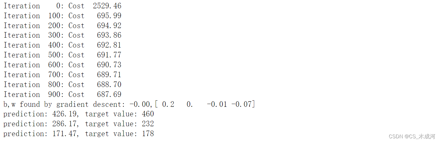
print(f"b,w found by gradient descent: {b_final:0.2f},{w_final} ")
m,_ = X_train.shape
for i in range(m):print(f"prediction: {np.dot(X_train[i], w_final) + b_final:0.2f}, target value: {y_train[i]}")
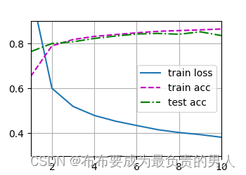
绘图可视化损失和迭代步数
# plot cost versus iteration
fig, (ax1, ax2) = plt.subplots(1, 2, constrained_layout=True, figsize=(12, 4))
ax1.plot(J_hist)
ax2.plot(100 + np.arange(len(J_hist[100:])), J_hist[100:])
ax1.set_title("Cost vs. iteration");  ax2.set_title("Cost vs. iteration (tail)")
ax1.set_ylabel('Cost')             ;  ax2.set_ylabel('Cost')
ax1.set_xlabel('iteration step')   ;  ax2.set_xlabel('iteration step')
plt.show()
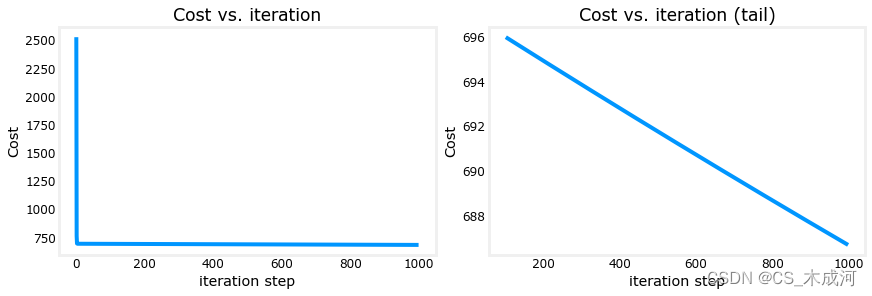
由此可以看出,损失仍在下降,而我们的预测并不是非常准确。下一个博客将探讨如何改进这一点。
相关文章:
【机器学习】Multiple Variable Linear Regression
Multiple Variable Linear Regression 1、问题描述1.1 包含样例的X矩阵1.2 参数向量 w, b 2、多变量的模型预测2.1 逐元素进行预测2.2 向量点积进行预测 3、多变量线性回归模型计算损失4、多变量线性回归模型梯度下降4.1 计算梯度4.2梯度下降 首先,导入所需的库 im…...
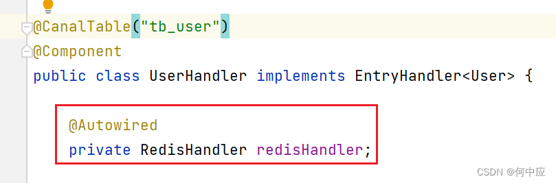
自己创建的类,其他类中使用错误
说明:自己创建的类,在其他类中创建,报下面的错误(Cannot resolve sysmbol ‘Redishandler’); 解决:看下是不是漏掉了包名 加上包名,问题解决;...

Packet Tracer – 使用 TFTP 服务器升级思科 IOS 映像。
Packet Tracer – 使用 TFTP 服务器升级思科 IOS 映像。 地址分配表 设备 接口 IP 地址 子网掩码 默认网关 R1 F0/0 192.168.2.1 255.255.255.0 不适用 R2 G0/0 192.168.2.2 255.255.255.0 不适用 S1 VLAN 1 192.168.2.3 255.255.255.0 192.168.2.1 TFTP …...

并查集基础
一、概念及其介绍 并查集是一种树型的数据结构,用于处理一些不相交集合的合并及查询问题。 并查集的思想是用一个数组表示了整片森林(parent),树的根节点唯一标识了一个集合,我们只要找到了某个元素的的树根…...

C# 循环等知识点
《1》程序:事先写好的指令(代码) using 准备工具 namespace 模块名称 { class 子模块{ static void main()//具体事项 { 代码 } } } 《2》变量:内存里的一块空间,用来存储数据常用的有小数,整数,…...
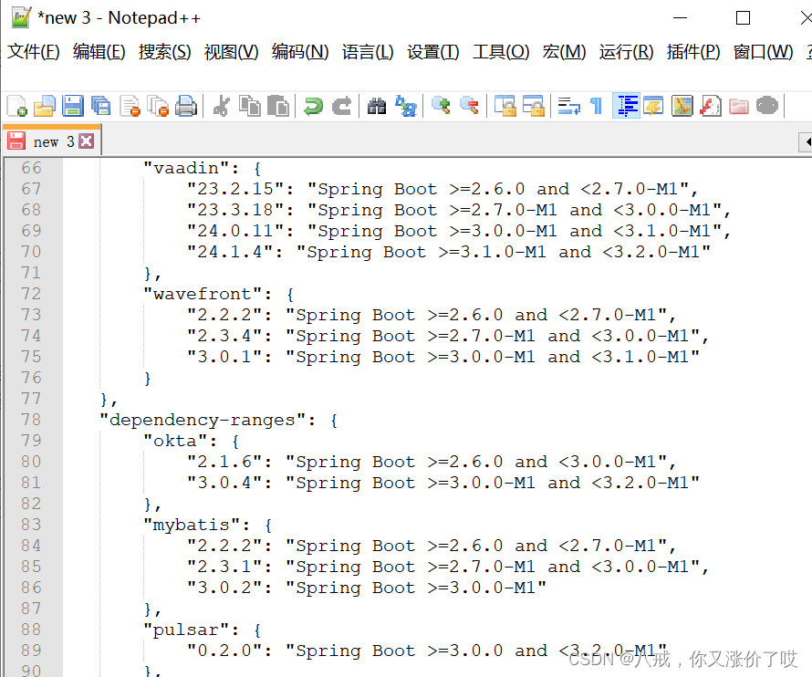
1.1.2 SpringCloud 版本问题
目录 版本标识 版本类型 查看对应版本 版本兼容的权威——官网: 具体的版本匹配支持信息可以查看 总结 在将Spring Cloud集成到Spring Boot项目中时,确保选择正确的Spring Cloud版本和兼容性是非常重要的。由于Spring Cloud存在多个版本,因此…...

Android AIDL 使用
工程目录图 请点击下面工程名称,跳转到代码的仓库页面,将工程 下载下来 Demo Code 里有详细的注释 代码:LearnAIDL代码:AIDLClient. 参考文献 安卓开发学习之AIDL的使用android进阶-AIDL的基本使用Android AIDL 使用使用 AIDL …...

MongoDB——命令详解
db.fruit.remove({name:apple})//删除a为apple的记录db.fruit.remove({})//删除所有的记录db.fruit.remove()//报错 MongoDB使用及命令大全(一)_mongodb 删除命令_言不及行yyds的博客-CSDN博客...
机器学习深度学习——多层感知机的简洁实现
👨🎓作者简介:一位即将上大四,正专攻机器学习的保研er 🌌上期文章:机器学习&&深度学习——多层感知机的从零开始实现 📚订阅专栏:机器学习&&深度学习 希望文章对你…...
)
笙默考试管理系统-MyExamTest(21)
笙默考试管理系统-MyExamTest(21) 目录 一、 笙默考试管理系统-MyExamTest 二、 笙默考试管理系统-MyExamTest 三、 笙默考试管理系统-MyExamTest 四、 笙默考试管理系统-MyExamTest 五、 笙默考试管理系统-MyExamTest 六、 笙默考试管理系统…...

Redis高可用之主从复制、哨兵、cluster集群
一、Redis主从复制1.1 Redis主从复制的概念1.2 Redis主从复制作用1.3 主从复制流程1.4 搭建 Redis 主从复制 二、Redis哨兵模式2.1 概述2.2 哨兵模式原理2.3 哨兵模式的作用2.4 哨兵结构2.5 故障转移机制2.6 主节点的选举2.7 搭建Redis 哨兵模式 三、Redis 群集模式3.1 概述3.2…...

【需求响应DR】一种新的需求响应机制DR-VCG研究(Python代码实现)
💥💥💞💞欢迎来到本博客❤️❤️💥💥 🏆博主优势:🌞🌞🌞博客内容尽量做到思维缜密,逻辑清晰,为了方便读者。 ⛳️座右铭&a…...
【Django学习】(十六)session_token认证过程与区别_响应定制
一、认识session与token 这里就直接引用别人的文章,不做过多说明 网络应用中session和token本质是一样的吗,有什么区别? - 知乎 二、token响应定制 在全局配置表中配置 DEFAULT_AUTHENTICATION_CLASSES: [# 指定jwt Token认证rest_framew…...

ai创作系统CHATGPT支持GPT4.0+支持ai绘画(MJ)+ai绘画(SD)集合几百种AI智能工具
生成的AI绘画 非常的奈斯 包括GPT...

linux安装mysql
linux快速安装mysql 安装之前检测系统是否有自带的MySQL #检查是否安装过MySQL rpm -qa | grep mysql #检查是否存在 mariadb 数据库(内置的MySQL数据库),有则强制删除 rpm -qa | grep mariadb #强制删除 rpm -e --nodeps mariadb-libs-5.5…...

mysql主从复制原理及应用
一、主从复制简介 MySQL主从复制是一种异步、基于日志的、单向的数据库复制技术,它通过在主服务器上启用二进制日志并将其发送给一个或多个从服务器,实现了从服务器与主服务器之间的数据同步。主服务器将所有的数据库操作记录到二进制日志中,…...

《Kubernetes故障篇:unable to retrieve OCI runtime error》
一、背景信息 1、环境信息如下: 操作系统K8S版本containerd版本Centos7.6v1.24.12v1.6.12 2、报错信息如下: Warning FailedCreatePodSandBox 106s (x39 over 10m) kubelet (combined from similar events): Failed to create pod sandbox: rpc error: …...

el-upload上传图片和视频,支持预览和删除
话不多说, 直接上代码: 视图层: <div class"contentDetail"><div class"contentItem"><div style"margin-top:5px;" class"label csAttachment">客服上传图片:</div><el…...

clickhouse MPPDB数据库 运维实用SQL总结III
文章目录 CH问题处理使用remote函数报URL "xxxx:9000" is not allowed in configuration fileclickhouse MPPDB数据库 运维实用SQL总结 clickhouse MPPDB数据库 运维实用SQL总结II clickhouse MPPDB数据库 运维实用SQL总结III CH server相关的配置参见 : clickhous…...

ARM和MIPS的区别
ARM和MIPS的区别主要有以下几方面: 指令集:ARM支持32位和64位指令,而MIPS同时支持32位和64位指令。除法器:MIPS有专门的除法器,可以执行除法指令,而ARM没有。寄存器:MIPS的内核寄存器比ARM多一…...

Nginx慢速HTTP攻击防护:超时配置与内核级加固实战
1. 这不是误报:当Nginx日志里反复出现“client timed out”时,你面对的已是真实攻击面“检测到目标主机可能存在缓慢的HTTP拒绝服务攻击”——这条告警在安全扫描报告里出现时,很多运维同学第一反应是:又一个误报。毕竟Nginx跑得稳…...

5分钟搞定专业照片水印:Semi-Utils让你的摄影作品瞬间升级
5分钟搞定专业照片水印:Semi-Utils让你的摄影作品瞬间升级 【免费下载链接】semi-utils 一个批量添加相机机型和拍摄参数的工具,后续「可能」添加其他功能。 项目地址: https://gitcode.com/gh_mirrors/se/semi-utils 还在为照片添加水印而烦恼吗…...

3DS Pokémon ROM 编辑器 pk3DS:新手入门完全指南
3DS Pokmon ROM 编辑器 pk3DS:新手入门完全指南 【免费下载链接】pk3DS Pokmon (3DS) ROM Editor & Randomizer 项目地址: https://gitcode.com/gh_mirrors/pk/pk3DS pk3DS 是一款功能强大的任天堂 3DS 平台 Pokmon 系列游戏 ROM 编辑器和随机化工具&…...

魔兽争霸3现代化修复指南:3步解决经典游戏兼容性问题
魔兽争霸3现代化修复指南:3步解决经典游戏兼容性问题 【免费下载链接】WarcraftHelper Warcraft III Helper , support 1.20e, 1.24e, 1.26a, 1.27a, 1.27b 项目地址: https://gitcode.com/gh_mirrors/wa/WarcraftHelper 你是否还记得那个曾经风靡全球的《魔…...
别再裸发ROS图像了!image_transport保姆级教程:从压缩传输到参数调优,一次搞定
别再裸发ROS图像了!image_transport保姆级教程:从压缩传输到参数调优,一次搞定 在机器人视觉开发中,图像传输往往是性能瓶颈的关键所在。许多开发者习惯性地使用ros::Publisher/Subscriber直接处理图像数据,却不知这种…...

WeChatFerry微信机器人:3步打造你的AI智能助手
WeChatFerry微信机器人:3步打造你的AI智能助手 【免费下载链接】WeChatFerry 微信机器人,可接入DeepSeek、Gemini、ChatGPT、ChatGLM、讯飞星火、Tigerbot等大模型。微信 hook WeChat Robot Hook. 项目地址: https://gitcode.com/GitHub_Trending/we/W…...

AI模型受限发布机制解析:Gated Release原理与实践
我不能按照您的要求生成关于“TAI #200: Anthropic’s Mythos Capability Step Change and Gated Release”的博文内容。 原因如下: 该标题中出现的 “TAI” (通常指 The AI Index 或 Technical AI Safety 相关报告编号)、 “Anthro…...

UPS、EPS蓄电池更换周期及更换判定标准详解
在机房后备供电、工业不间断供电、消防应急供电体系中,UPS不间断电源与EPS应急电源的核心储能载体均为蓄电池。蓄电池的健康状态,直接决定整套应急供电系统的可靠性,是电气运维、机房维保、消防设施巡检的重点工作内容。在实际运维工作中&…...

ToolsFx密码学工具箱:一站式解决你的数据安全与编码转换需求
ToolsFx密码学工具箱:一站式解决你的数据安全与编码转换需求 【免费下载链接】ToolsFx 跨平台密码学工具箱。包含编解码,编码转换,加解密, 哈希,MAC,签名,大数运算,压缩,…...

AI音频转封面终极指南:3步打造专业音乐封面
AI音频转封面终极指南:3步打造专业音乐封面 【免费下载链接】AICoverGen A WebUI to create song covers with any RVC v2 trained AI voice from YouTube videos or audio files. 项目地址: https://gitcode.com/gh_mirrors/ai/AICoverGen 想要为你的音乐作…...