pytorch
PyTorch基础
import torch
torch.__version__ #return '1.13.1+cu116'
基本使用方法
矩阵
x = torch.empty(5, 3)tensor([[1.4586e-19, 1.1578e+27, 2.0780e-07],[6.0542e+22, 7.8675e+34, 4.6894e+27],[1.6217e-19, 1.4333e-19, 2.7530e+12],[7.5338e+28, 8.1173e-10, 4.3861e-43],[2.8912e-03, 4.3861e-43, 2.8912e-03]])随机值
x = torch.rand(5, 3)#5行三列的随机值tensor([[0.1511, 0.6433, 0.1245],[0.8949, 0.8577, 0.3564],[0.7810, 0.5037, 0.7101],[0.1997, 0.4917, 0.1746],[0.4288, 0.9921, 0.4862]])
初始化一个全零的矩阵
x = torch.zeros(5, 3, dtype=torch.long)tensor([[0, 0, 0],[0, 0, 0],[0, 0, 0],[0, 0, 0],[0, 0, 0]])
直接传入数据
x = torch.tensor([5.5, 3])
tensor([5.5000, 3.0000])
x = x.new_ones(5, 3, dtype=torch.double)    tensor([[1., 1., 1.],[1., 1., 1.],[1., 1., 1.],[1., 1., 1.],[1., 1., 1.]], dtype=torch.float64)
x = torch.randn_like(x, dtype=torch.float) #返回一个x大小相同的张量,其由均值为0、方差为1的标准正态分布填充tensor([[ 0.6811, -1.2104, -1.2676],[-0.3295,  0.1155, -0.5736],[-1.3656, -0.4973, -0.7043],[-1.3670, -0.3296,  3.1743],[ 1.3443,  0.3373,  0.6182]])
展示矩阵大小
x.size()torch.Size([5, 3])
基本计算方法
y = torch.rand(5, 3)#随机5行三列矩阵tensor([[0.0542, 0.9674, 0.5902],[0.7749, 0.1682, 0.2871],[0.1747, 0.3728, 0.2077],[0.9092, 0.3087, 0.3981],[0.4231, 0.8725, 0.6005]])
x		        tensor([[ 0.6811, -1.2104, -1.2676],[-0.3295,  0.1155, -0.5736],[-1.3656, -0.4973, -0.7043],[-1.3670, -0.3296,  3.1743],[ 1.3443,  0.3373,  0.6182]])
x + ytensor([[ 0.7353, -0.2430, -0.6774],[ 0.4454,  0.2837, -0.2865],[-1.1908, -0.1245, -0.4967],[-0.4578, -0.0209,  3.5723],[ 1.7674,  1.2098,  1.2187]])
torch.add(x, y)#一样的也是加法tensor([[ 0.7353, -0.2430, -0.6774],[ 0.4454,  0.2837, -0.2865],[-1.1908, -0.1245, -0.4967],[-0.4578, -0.0209,  3.5723],[ 1.7674,  1.2098,  1.2187]])
索引
x[:, 1]tensor([-1.2104, 0.1155, -0.4973, -0.3296, 0.3373])
x.view() 类似于reshape(),重塑维度
x = torch.randn(4, 4)tensor([[ 0.1811, -1.4025, -1.2865, -1.6370],[-0.2279,  1.0993, -0.4067, -0.2652],[-0.5673,  0.2697,  1.8822, -1.3748],[-0.3731, -0.9595,  1.8725, -0.8774]])
y = x.view(16)tensor([-0.3035, -2.5819,  1.2449, -0.3448,  1.0095, -0.1734,  1.5666,  0.5170,-1.0587,  0.1241, -0.5550, -1.6905,  0.8625, -1.3681, -0.1491,  0.2202])
z = x.view(-1, 8) #-1是值得注意的,x中总共16个元素,现在定义一行是8列(8个元素),16/8 = 2,所以是2行tensor([[-0.3035, -2.5819,  1.2449, -0.3448,  1.0095, -0.1734,  1.5666,  0.5170],[-1.0587,  0.1241, -0.5550, -1.6905,  0.8625, -1.3681, -0.1491,  0.2202]])
print(x.size(), y.size(), z.size())torch.Size([4, 4]) torch.Size([16]) torch.Size([2, 8])
与Numpy的协同操作(互转)
a = torch.ones(5)tensor([1., 1., 1., 1., 1.])
b = a.numpy()array([1., 1., 1., 1., 1.], dtype=float32)import numpy as np
a = np.ones(5)array([1., 1., 1., 1., 1.])
b = torch.from_numpy(a)tensor([1., 1., 1., 1., 1.], dtype=torch.float64)
autograb机制
需要求导的,可以手动定义:
x = torch.randn(3,4)#torch.randn:用来生成随机数字的tensor,这些随机数字满足标准正态分布(0~1)tensor([[-1.5885,  0.6992, -0.2198,  1.2736],[ 0.6211, -0.3729,  0.1261,  1.4094],[ 0.7418, -0.2801, -0.0672, -0.5614]])
x = torch.randn(3,4,requires_grad=True)tensor([[ 0.9318, -1.0761,  0.6794,  1.2261],[-1.7192, -0.6009, -0.3852,  0.2492],[-0.1853,  0.2066,  0.9497, -0.3329]], requires_grad=True)
#方法2
x = torch.randn(3,4)
x.requires_grad=Truetensor([[-1.9635,  0.5769,  1.2705, -0.8758],[ 1.2847, -1.0498, -0.3650, -0.5059],[ 0.2780,  0.0816,  0.7754,  0.2048]], requires_grad=True)
b = torch.randn(3,4,requires_grad=True)
t = x + b
y = t.sum()tensor(4.4444, grad_fn=<SumBackward0>)
y.backward()
b.gradtensor([[1., 1., 1., 1.],[1., 1., 1., 1.],[1., 1., 1., 1.]])
虽然没有指定t的requires_grad但是需要用到它,也会默认的
x.requires_grad, b.requires_grad, t.requires_grad#return (True, True, True) 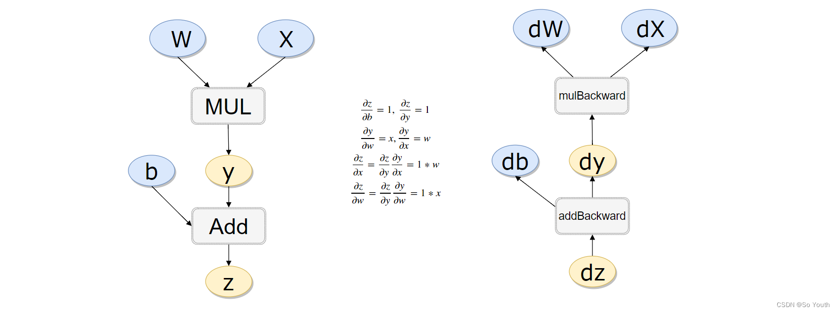
#计算流程
x = torch.rand(1)
b = torch.rand(1, requires_grad = True)
w = torch.rand(1, requires_grad = True)
y = w * x
z = y + b
x.requires_grad, b.requires_grad, w.requires_grad, y.requires_grad#注意y也是需要的(False, True, True, True)
x.is_leaf, w.is_leaf, b.is_leaf, y.is_leaf, z.is_leaf(True, True, True, False, False)
返向传播计算
z.backward(retain_graph=True)#如果不清空会累加起来
w.grad 累加后的结果tensor([1.6244])
b.gradtensor([2.])
做一个线性回归
构造一组输入数据X和其对应的标签y
x_values = [i for i in range(11)]
x_train = np.array(x_values, dtype=np.float32)
x_train = x_train.reshape(-1, 1)
x_train.shape #return (11, 1)y_values = [2*i + 1 for i in x_values]
y_train = np.array(y_values, dtype=np.float32)
y_train = y_train.reshape(-1, 1)
y_train.shape# (11, 1)import torch
import torch.nn as nn
线性回归模型:其实线性回归就是一个不加激活函数的全连接层
class LinearRegressionModel(nn.Module):def __init__(self, input_dim, output_dim):super(LinearRegressionModel, self).__init__()self.linear = nn.Linear(input_dim, output_dim)  def forward(self, x):#前向传播out = self.linear(x)return out
input_dim = 1
output_dim = 1model = LinearRegressionModel(input_dim, output_dim)LinearRegressionModel((linear): Linear(in_features=1, out_features=1, bias=True))
指定好参数和损失函数
epochs = 1000  #执行次数
learning_rate = 0.01 #准确率
optimizer = torch.optim.SGD(model.parameters(), lr=learning_rate)#优化模型
criterion = nn.MSELoss()#绝对值损失函数是计算预测值与目标值的差的绝对值
训练模型
for epoch in range(epochs):epoch += 1# 注意转行成tensorinputs = torch.from_numpy(x_train)labels = torch.from_numpy(y_train)# 梯度要清零每一次迭代optimizer.zero_grad() # 前向传播outputs = model(inputs)# 计算损失loss = criterion(outputs, labels)# 返向传播loss.backward()# 更新权重参数optimizer.step()if epoch % 50 == 0:print('epoch {}, loss {}'.format(epoch, loss.item()))epoch 50, loss 0.4448287785053253epoch 100, loss 0.25371354818344116epoch 150, loss 0.14470864832401276epoch 200, loss 0.08253632485866547epoch 250, loss 0.04707561805844307epoch 300, loss 0.026850251480937004epoch 350, loss 0.015314370393753052epoch 400, loss 0.008734731003642082epoch 450, loss 0.004981952253729105epoch 500, loss 0.002841521752998233epoch 550, loss 0.0016206930158659816epoch 600, loss 0.0009243797394447029epoch 650, loss 0.0005272324196994305epoch 700, loss 0.0003007081104442477epoch 750, loss 0.00017151293286588043epoch 800, loss 9.782632696442306e-05epoch 850, loss 5.579544449574314e-05epoch 900, loss 3.182474029017612e-05epoch 950, loss 1.8151076801586896e-05epoch 1000, loss 1.0352457138651516e-05
测试模型预测结果
predicted = model(torch.from_numpy(x_train).requires_grad_()).data.numpy()array([[ 0.99918383],[ 2.9993014 ],[ 4.9994187 ],[ 6.9995365 ],[ 8.999654  ],[10.999771  ],[12.999889  ],[15.000007  ],[17.000124  ],[19.000242  ],[21.000359  ]], dtype=float32)
模型的保存与读取
torch.save(model.state_dict(), 'model.pkl')
model.load_state_dict(torch.load('model.pkl'))<All keys matched successfully>
使用GPU进行训练:只需要把数据和模型传入到cuda里面就可以了
import torch
import torch.nn as nn
import numpy as npclass LinearRegressionModel(nn.Module):def __init__(self, input_dim, output_dim):super(LinearRegressionModel, self).__init__()self.linear = nn.Linear(input_dim, output_dim)  def forward(self, x):out = self.linear(x)return outinput_dim = 1
output_dim = 1model = LinearRegressionModel(input_dim, output_dim)######使用GPU还是CPU
device = torch.device("cuda:0" if torch.cuda.is_available() else "cpu")
model.to(device)criterion = nn.MSELoss()learning_rate = 0.01optimizer = torch.optim.SGD(model.parameters(), lr=learning_rate)epochs = 1000
for epoch in range(epochs):epoch += 1####加上.to(device)inputs = torch.from_numpy(x_train).to(device)labels = torch.from_numpy(y_train).to(device)optimizer.zero_grad() outputs = model(inputs)loss = criterion(outputs, labels)loss.backward()optimizer.step()if epoch % 50 == 0:print('epoch {}, loss {}'.format(epoch, loss.item()))epoch 50, loss 0.011100251227617264epoch 100, loss 0.006331132724881172epoch 150, loss 0.003611058695241809epoch 200, loss 0.0020596047397702932epoch 250, loss 0.0011747264070436358epoch 300, loss 0.0006700288504362106epoch 350, loss 0.00038215285167098045epoch 400, loss 0.00021796672081109136epoch 450, loss 0.00012431896175257862epoch 500, loss 7.090995495673269e-05epoch 550, loss 4.044298475491814e-05epoch 600, loss 2.3066799258231185e-05epoch 650, loss 1.3156819477444515e-05epoch 700, loss 7.503344477299834e-06epoch 750, loss 4.279831500753062e-06epoch 800, loss 2.4414177914877655e-06epoch 850, loss 1.3924694712841301e-06epoch 900, loss 7.945647553242452e-07epoch 950, loss 4.530382398115762e-07epoch 1000, loss 2.5830334493548435e-07
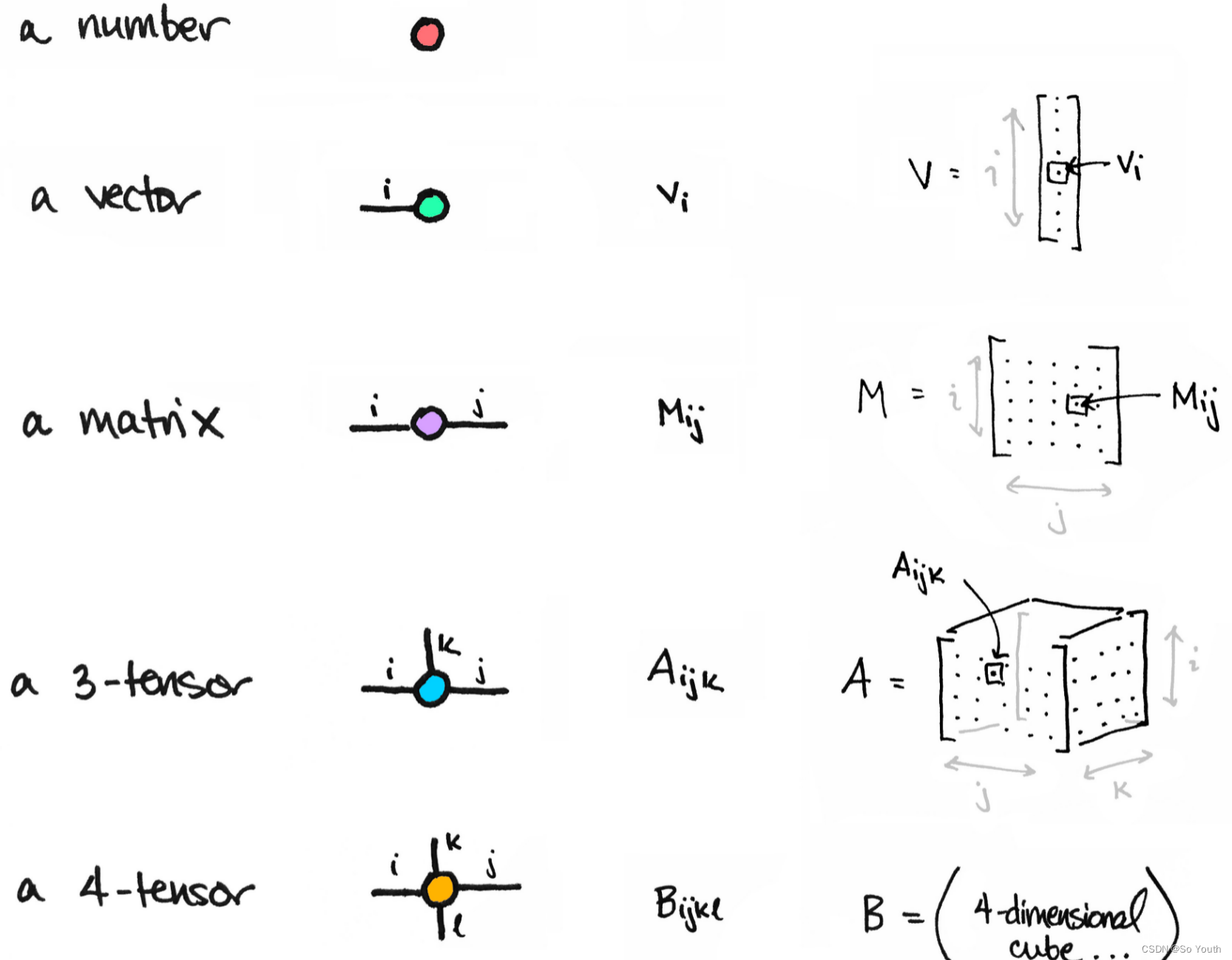
Tensor常见的形式
0: scalar:通常就是一个数值
1: vector:例如: [-5., 2., 0.],在深度学习中通常指特征,例如词向量特征,某一维度特征等
2: matrix:一般计算的都是矩阵,通常都是多维的
3: n-dimensional tensor:
Scalar
x = tensor(42.)tensor(42.)
x.dim()0
Vector
一维向量
v = tensor([1.5, -0.5, 3.0])tensor([ 1.5000, -0.5000,  3.0000])
v.dim()1
v.size()torch.Size([3])
Matrix
M = tensor([[1., 2.], [3., 4.]])tensor([[1., 2.],[3., 4.]])
M.matmul(M)#矩阵乘法tensor([[ 7., 10.],[15., 22.]])
几种形状的Tensor
强大hub模块
GITHUB:https://github.com/pytorch/hub
模型:https://pytorch.org/hub/research-modelsimport torch
model = torch.hub.load('pytorch/vision:v0.4.2', 'deeplabv3_resnet101', pretrained=True)
model.eval()torch.hub.list('pytorch/vision:v0.4.2')# Download an example image from the pytorch website
import urllib
url, filename = ("https://github.com/pytorch/hub/raw/master/dog.jpg", "dog.jpg")
try: urllib.URLopener().retrieve(url, filename)
except: urllib.request.urlretrieve(url, filename)# sample execution (requires torchvision)
from PIL import Image
from torchvision import transforms
input_image = Image.open(filename)
preprocess = transforms.Compose([transforms.ToTensor(),transforms.Normalize(mean=[0.485, 0.456, 0.406], std=[0.229, 0.224, 0.225]),
])input_tensor = preprocess(input_image)
input_batch = input_tensor.unsqueeze(0) # create a mini-batch as expected by the model# move the input and model to GPU for speed if available
if torch.cuda.is_available():input_batch = input_batch.to('cuda')model.to('cuda')with torch.no_grad():output = model(input_batch)['out'][0]
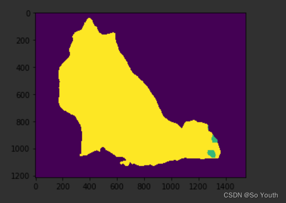
output_predictions = output.argmax(0)# create a color pallette, selecting a color for each class
palette = torch.tensor([2 ** 25 - 1, 2 ** 15 - 1, 2 ** 21 - 1])
colors = torch.as_tensor([i for i in range(21)])[:, None] * palette
colors = (colors % 255).numpy().astype("uint8")# plot the semantic segmentation predictions of 21 classes in each color
r = Image.fromarray(output_predictions.byte().cpu().numpy()).resize(input_image.size)
r.putpalette(colors)import matplotlib.pyplot as plt
plt.imshow(r)
plt.show()
神经网络实战分类与回归任务
神经网络进行气温预测
import numpy as np
import pandas as pd
import matplotlib.pyplot as plt
import torch
import torch.optim as optim
import warnings
warnings.filterwarnings("ignore")
%matplotlib inline
#(1)数据获取
features = pd.read_csv('temps.csv')
#看看数据长什么样子
features.head()
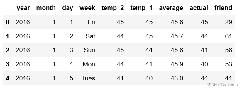
print('数据维度:', features.shape)#数据维度: (348, 9)
# 处理时间数据
import datetime
# 分别得到年,月,日
years = features['year']
months = features['month']
days = features['day']# datetime格式
dates = [str(int(year)) + '-' + str(int(month)) + '-' + str(int(day)) for year, month, day in zip(years, months, days)]
dates = [datetime.datetime.strptime(date, '%Y-%m-%d') for date in dates]dates[:5][datetime.datetime(2016, 1, 1, 0, 0),datetime.datetime(2016, 1, 2, 0, 0),datetime.datetime(2016, 1, 3, 0, 0),datetime.datetime(2016, 1, 4, 0, 0),datetime.datetime(2016, 1, 5, 0, 0)]# 准备画图
# 指定默认风格
plt.style.use('fivethirtyeight')# 设置布局
fig, ((ax1, ax2), (ax3, ax4)) = plt.subplots(nrows=2, ncols=2, figsize = (10,10))
fig.autofmt_xdate(rotation = 45)# 标签值
ax1.plot(dates, features['actual'])
ax1.set_xlabel(''); ax1.set_ylabel('Temperature'); ax1.set_title('Max Temp')# 昨天
ax2.plot(dates, features['temp_1'])
ax2.set_xlabel(''); ax2.set_ylabel('Temperature'); ax2.set_title('Previous Max Temp')# 前天
ax3.plot(dates, features['temp_2'])
ax3.set_xlabel('Date'); ax3.set_ylabel('Temperature'); ax3.set_title('Two Days Prior Max Temp')# 我的逗逼朋友
ax4.plot(dates, features['friend'])
ax4.set_xlabel('Date'); ax4.set_ylabel('Temperature'); ax4.set_title('Friend Estimate')plt.tight_layout(pad=2)
# 独热编码  将字符串转化为特定的数字,数字编码
features = pd.get_dummies(features)
features.head(5)
# 标签
labels = np.array(features['actual'])# 在特征中去掉标签
features= features.drop('actual', axis = 1)# 名字单独保存一下,以备后患
feature_list = list(features.columns)# 转换成合适的格式
features = np.array(features)
features.shape#(348, 14)from sklearn import preprocessing
input_features = preprocessing.StandardScaler().fit_transform(features)
input_features[0]array([ 0.        , -1.5678393 , -1.65682171, -1.48452388, -1.49443549,-1.3470703 , -1.98891668,  2.44131112, -0.40482045, -0.40961596,-0.40482045, -0.40482045, -0.41913682, -0.40482045])
构建网络模型
x = torch.tensor(input_features, dtype = float)y = torch.tensor(labels, dtype = float)# 权重参数初始化
weights = torch.randn((14, 128), dtype = float, requires_grad = True)
biases = torch.randn(128, dtype = float, requires_grad = True)
weights2 = torch.randn((128, 1), dtype = float, requires_grad = True)
biases2 = torch.randn(1, dtype = float, requires_grad = True) learning_rate = 0.001
losses = []for i in range(1000):# 计算隐层hidden = x.mm(weights) + biases# 加入激活函数hidden = torch.relu(hidden)# 预测结果predictions = hidden.mm(weights2) + biases2# 通计算损失loss = torch.mean((predictions - y) ** 2) losses.append(loss.data.numpy())# 打印损失值if i % 100 == 0:print('loss:', loss)#返向传播计算loss.backward()#更新参数weights.data.add_(- learning_rate * weights.grad.data)  biases.data.add_(- learning_rate * biases.grad.data)weights2.data.add_(- learning_rate * weights2.grad.data)biases2.data.add_(- learning_rate * biases2.grad.data)# 每次迭代都得记得清空weights.grad.data.zero_()biases.grad.data.zero_()weights2.grad.data.zero_()biases2.grad.data.zero_()loss: tensor(8347.9924, dtype=torch.float64, grad_fn=<MeanBackward0>)loss: tensor(152.3170, dtype=torch.float64, grad_fn=<MeanBackward0>)loss: tensor(145.9625, dtype=torch.float64, grad_fn=<MeanBackward0>)loss: tensor(143.9453, dtype=torch.float64, grad_fn=<MeanBackward0>)loss: tensor(142.8161, dtype=torch.float64, grad_fn=<MeanBackward0>)loss: tensor(142.0664, dtype=torch.float64, grad_fn=<MeanBackward0>)loss: tensor(141.5386, dtype=torch.float64, grad_fn=<MeanBackward0>)loss: tensor(141.1528, dtype=torch.float64, grad_fn=<MeanBackward0>)loss: tensor(140.8618, dtype=torch.float64, grad_fn=<MeanBackward0>)loss: tensor(140.6318, dtype=torch.float64, grad_fn=<MeanBackward0>)
predictions.shape #torch.Size([348, 1])
更简单的构建网络模型
input_size = input_features.shape[1]
hidden_size = 128
output_size = 1
batch_size = 16
my_nn = torch.nn.Sequential(torch.nn.Linear(input_size, hidden_size),torch.nn.Sigmoid(),torch.nn.Linear(hidden_size, output_size),
)
cost = torch.nn.MSELoss(reduction='mean')
optimizer = torch.optim.Adam(my_nn.parameters(), lr = 0.001)# 训练网络
losses = []
for i in range(1000):batch_loss = []# MINI-Batch方法来进行训练for start in range(0, len(input_features), batch_size):end = start + batch_size if start + batch_size < len(input_features) else len(input_features)xx = torch.tensor(input_features[start:end], dtype = torch.float, requires_grad = True)yy = torch.tensor(labels[start:end], dtype = torch.float, requires_grad = True)prediction = my_nn(xx)loss = cost(prediction, yy)optimizer.zero_grad()loss.backward(retain_graph=True)optimizer.step()batch_loss.append(loss.data.numpy())# 打印损失if i % 100==0:losses.append(np.mean(batch_loss))print(i, np.mean(batch_loss))0 3950.7627100 37.9201200 35.654438300 35.278366400 35.116814500 34.986076600 34.868954700 34.75414800 34.637356900 34.516705
预测训练结果
x = torch.tensor(input_features, dtype = torch.float)
predict = my_nn(x).data.numpy()# 转换日期格式
dates = [str(int(year)) + '-' + str(int(month)) + '-' + str(int(day)) for year, month, day in zip(years, months, days)]
dates = [datetime.datetime.strptime(date, '%Y-%m-%d') for date in dates]# 创建一个表格来存日期和其对应的标签数值
true_data = pd.DataFrame(data = {'date': dates, 'actual': labels})# 同理,再创建一个来存日期和其对应的模型预测值
months = features[:, feature_list.index('month')]
days = features[:, feature_list.index('day')]
years = features[:, feature_list.index('year')]test_dates = [str(int(year)) + '-' + str(int(month)) + '-' + str(int(day)) for year, month, day in zip(years, months, days)]test_dates = [datetime.datetime.strptime(date, '%Y-%m-%d') for date in test_dates]predictions_data = pd.DataFrame(data = {'date': test_dates, 'prediction': predict.reshape(-1)}) # 真实值
plt.plot(true_data['date'], true_data['actual'], 'b-', label = 'actual')# 预测值
plt.plot(predictions_data['date'], predictions_data['prediction'], 'ro', label = 'prediction')
plt.xticks(rotation = '60');
plt.legend()# 图名
plt.xlabel('Date'); plt.ylabel('Maximum Temperature (F)'); plt.title('Actual and Predicted Values');
神经网络分类任务
Mnist分类任务

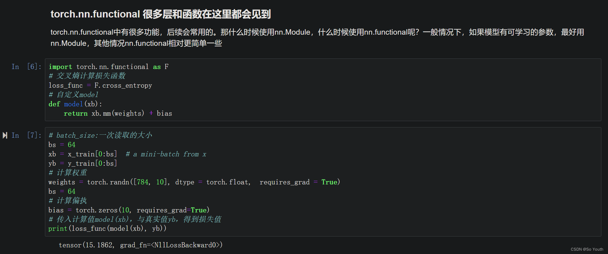
torch.nn.functional
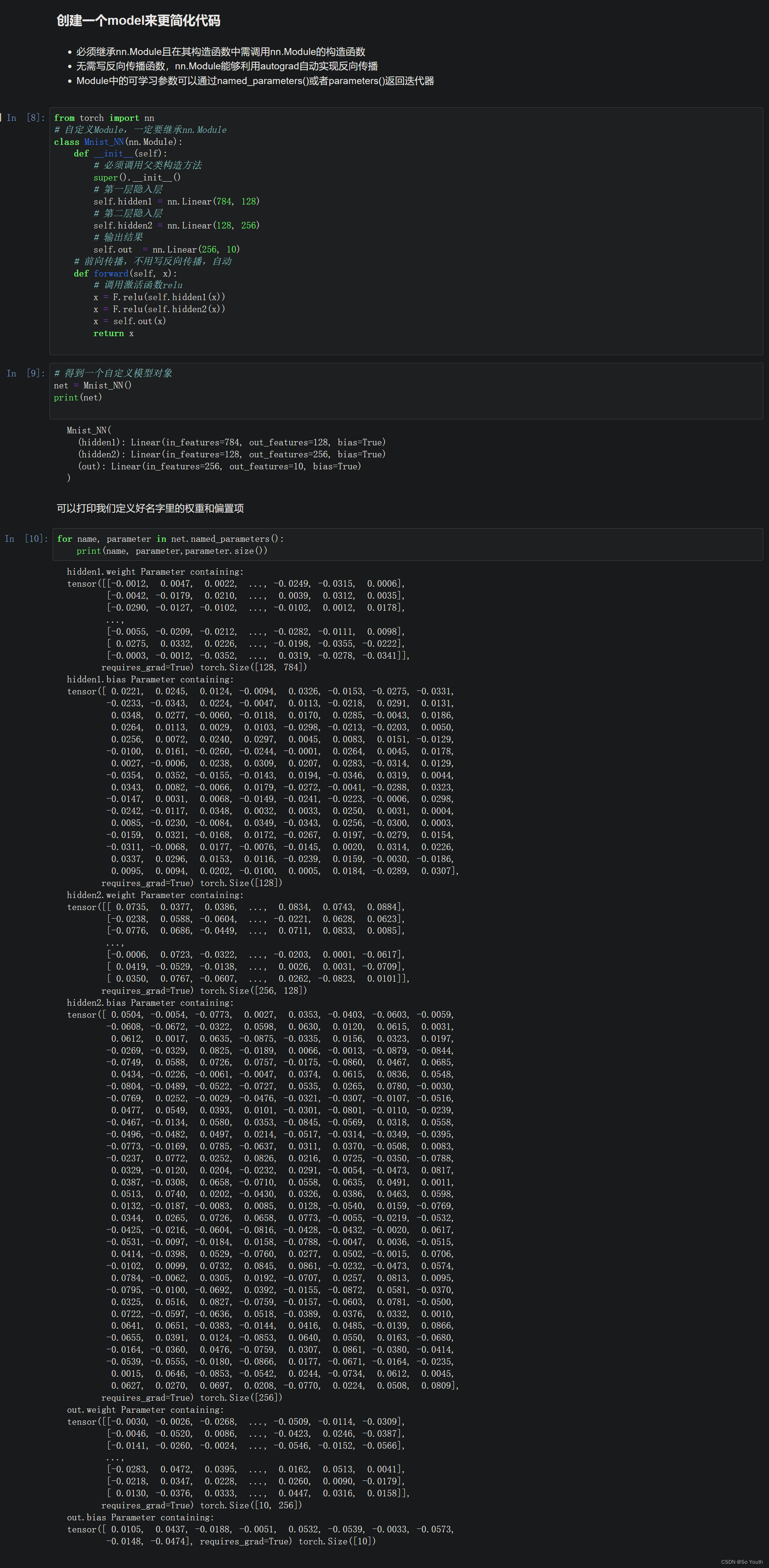
创建一个model来更简化代码
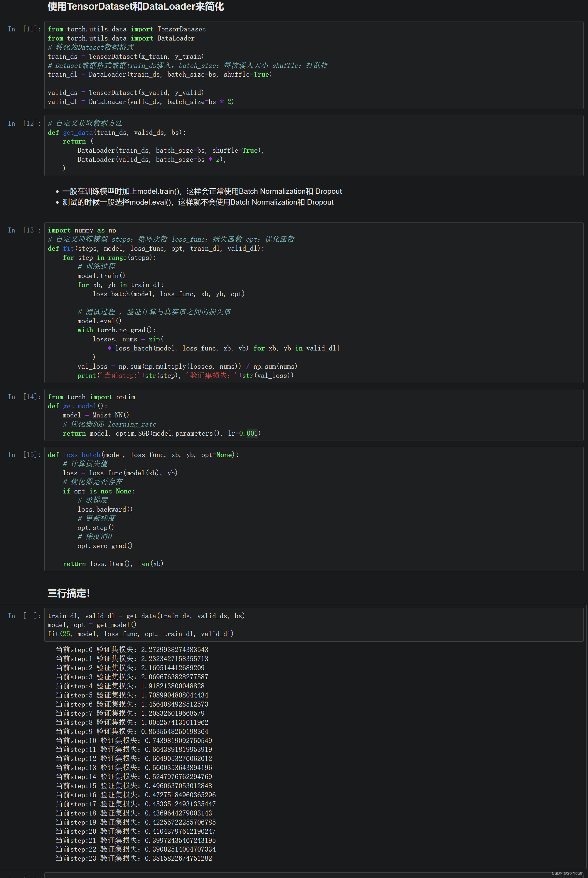
使用TensorDataset和DataLoader来简化
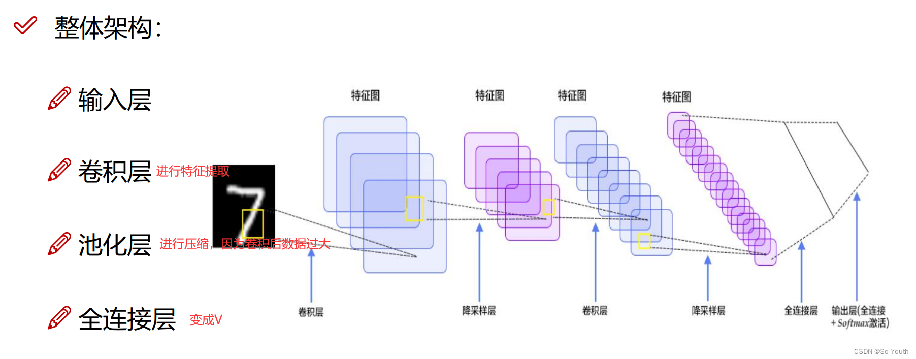
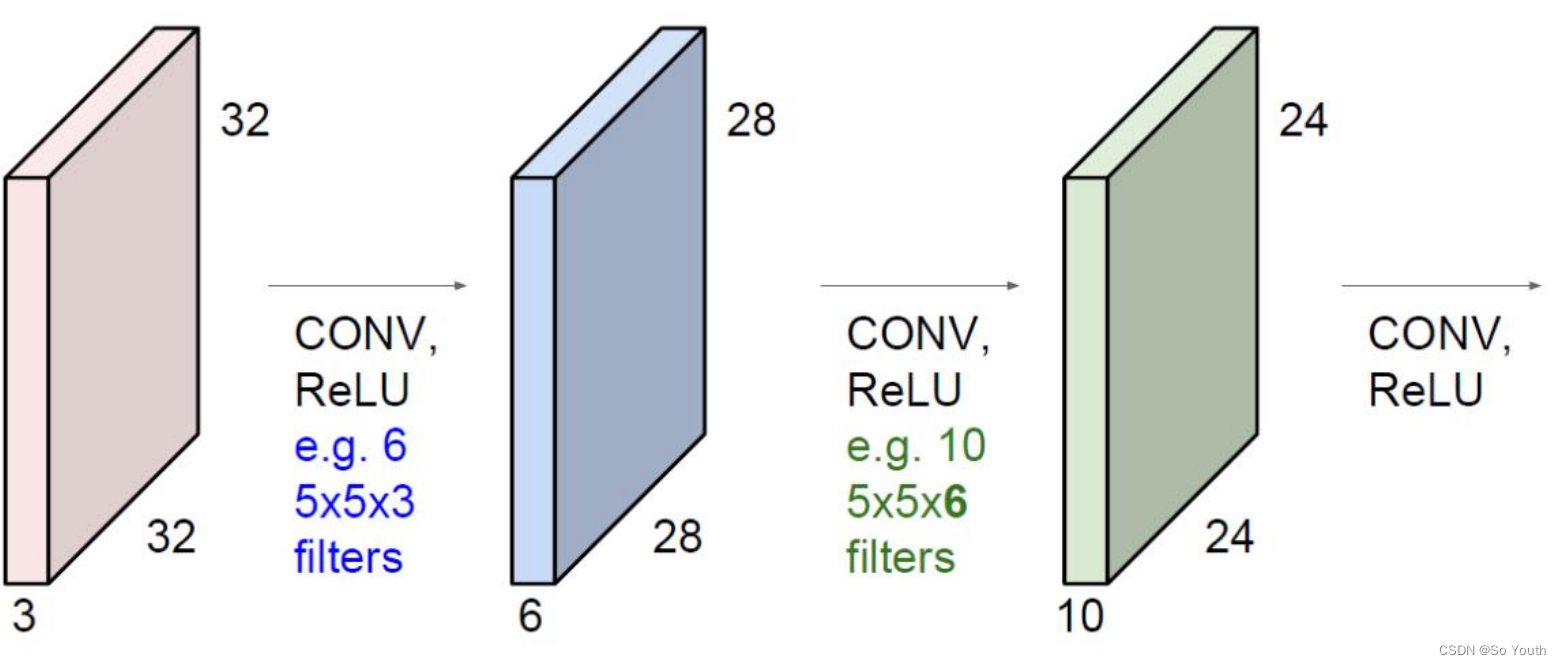
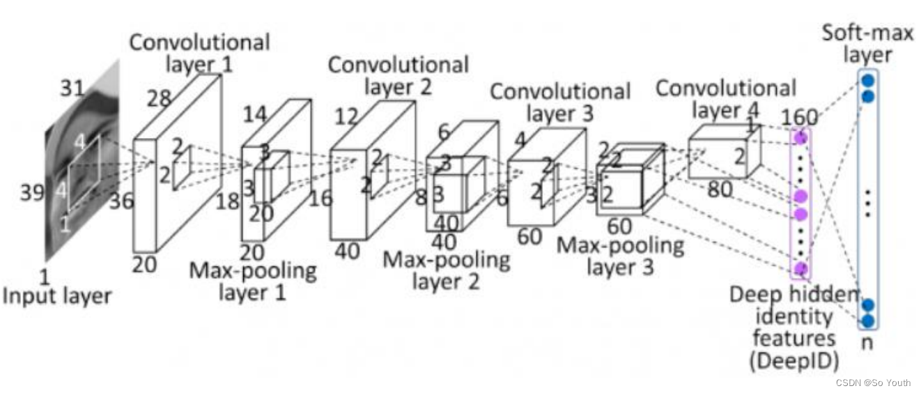
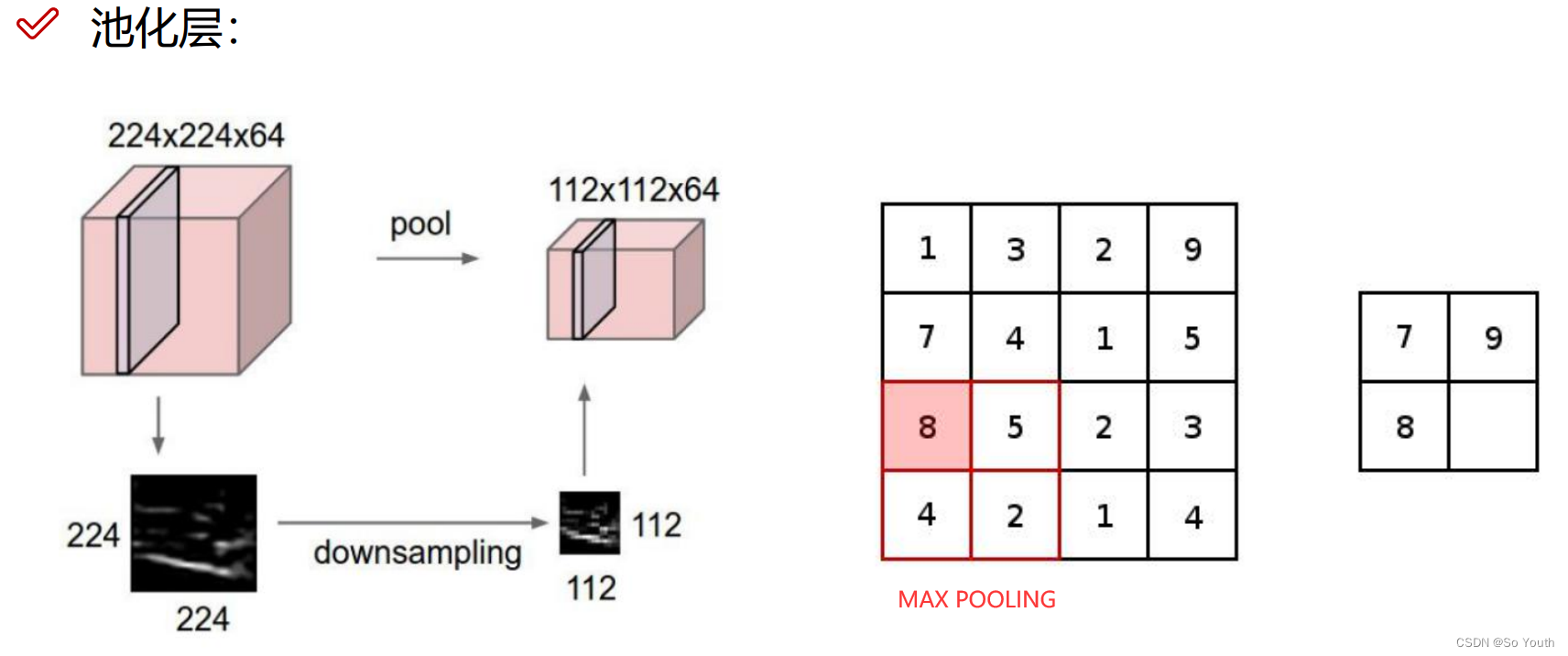
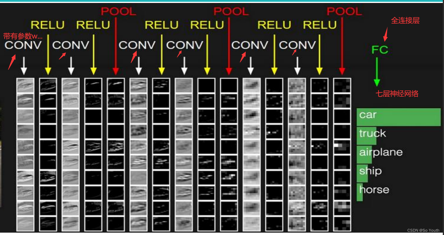
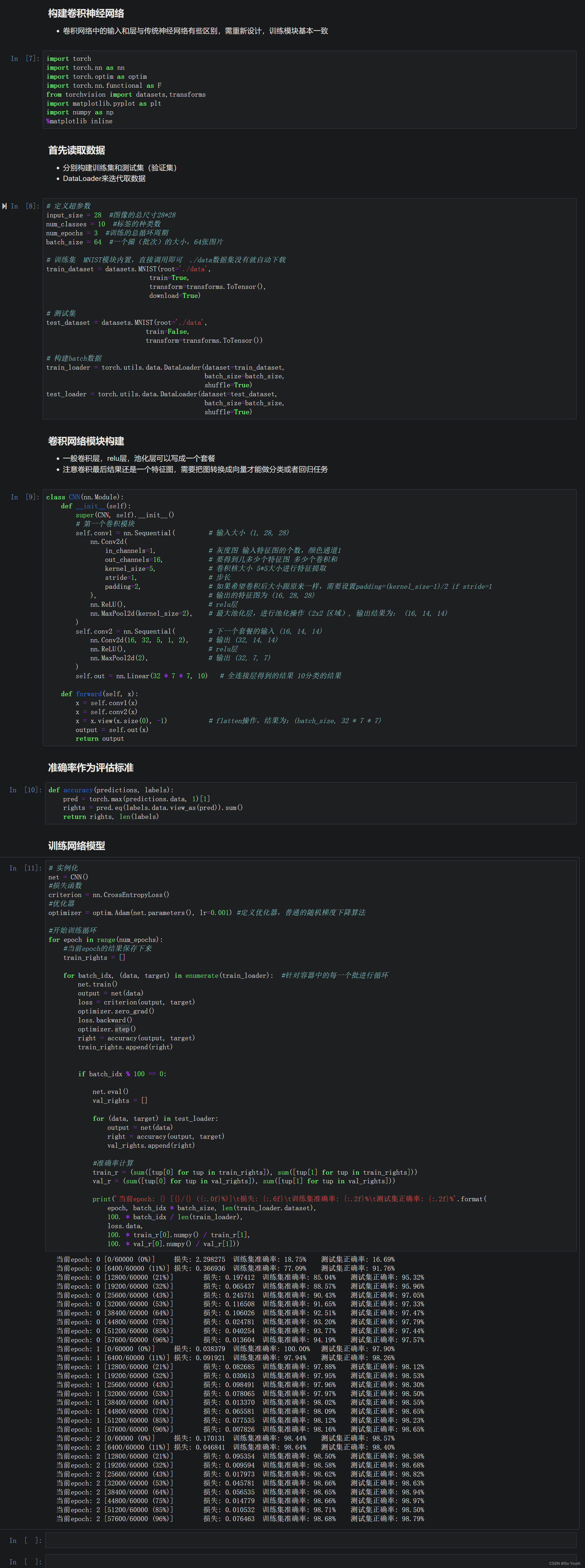
卷积神经网络

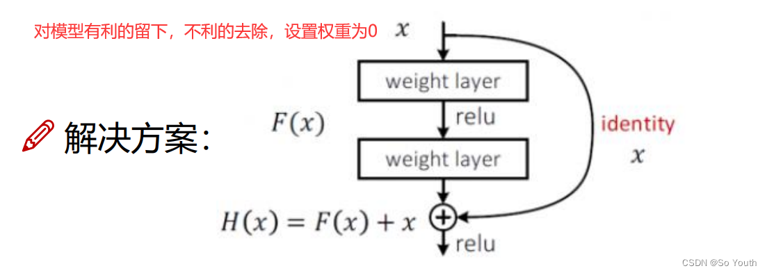
残差网络 (ResNets)
卷积神经网络效果(conv) cnn
相关文章:
pytorch
PyTorch基础 import torch torch.__version__ #return 1.13.1cu116基本使用方法 矩阵 x torch.empty(5, 3)tensor([[1.4586e-19, 1.1578e27, 2.0780e-07],[6.0542e22, 7.8675e34, 4.6894e27],[1.6217e-19, 1.4333e-19, 2.7530e12],[7.5338e28, 8.1173e-10, 4.3861e-43],[2.…...

软件测试—对职业生涯发展的一些感想
目录:导读 职场生涯 1、短期规划 2、长期规划 自身定位 1、你在哪儿? 2、你想要什么? 3、你拥有什么? 4、你需要做什么?什么时候做? 5、淡定啊淡定 最近工作不是很忙,有空都是在看书&a…...

5年经验之谈:月薪3000到30000,测试工程师的变“行”记!
自我介绍下,我是一名转IT测试人,我的专业是化学,去化工厂实习才发现这专业的坑人之处,化学试剂害人不浅,有毒,易燃易爆,实验室经常用丙酮,甲醇,四氯化碳,接触…...

全价值链赋能,数字化助力营销价值全力释放 | 爱分析报告
报告编委 张扬 爱分析联合创始人&首席分析师 文鸿伟 爱分析高级分析师 王鹏 爱分析分析师 外部专家(按姓氏拼音排序) 黄洵 客易达 联合创始人 毛健 云徙科技 副总裁 & COO 特别鸣谢(按拼音排序) 报告摘要 在…...
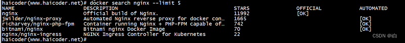
【自学Docker 】Docker search命令
大纲 Docker search命令 docker search命令教程 docker search 命令用于从 Docker Hub 查找镜像。 docker search命令语法 haicoder(www.haicoder.net)# docker search [OPTIONS] TERMdocker search命令参数 参数描述docker search --filter设置过滤条件。docker search -…...

银行零售如何更贴近客户?是时候升级你的客户旅程平台了
随着数字化战略推进,各大银行持续加大对线上多渠道的建设投入,客户触达也愈发移动化、智能化。与此同时,手机银行飞速发展产生并累积了大量客户行为数据,呈多样化、海量化等特点,将在用户体验、客户经营、手机银行运营…...
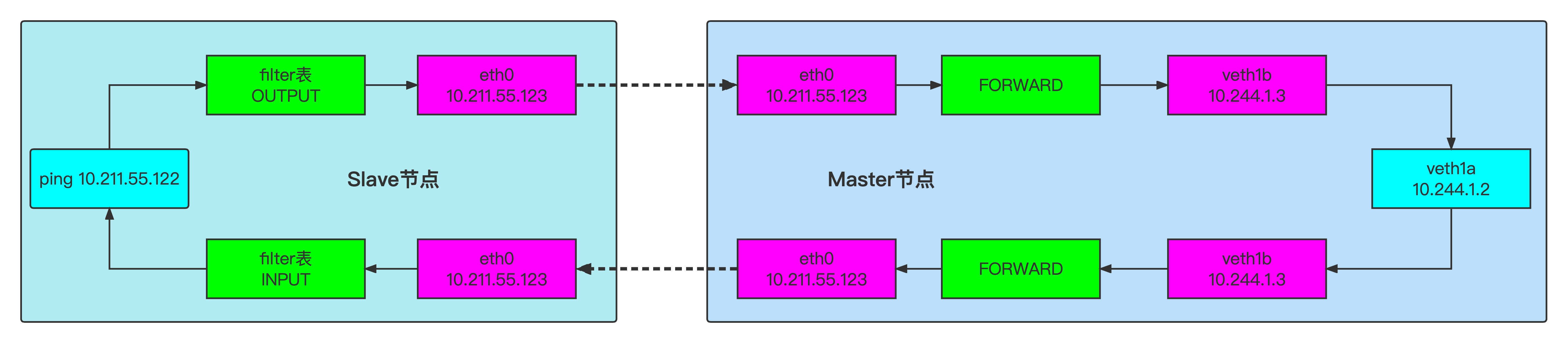
零入门kubernetes网络实战-12->基于DNAT技术使得外网可以访问本宿主机上veth-pair链接的内部网络
视频地址(稍后上传) 本篇文章测试如何让veth pair链接的内网网络可以被本局域网的其他宿主机访问到? 1、测试环境介绍 一台centos虚拟机 # 查看操作系统版本 cat /etc/centos-release # 内核版本 uname -a uname -r # 查看网卡信息 ip a s eth02、网络拓扑 3、操…...

conda环境管理命令
conda环境管理命令 1.环境检查 1)查看安装了哪些包 conda list 2)查看当前存在哪些虚拟环境 conda env list conda info -e [rootoracledb anaconda3]# conda info -e # conda environments: # base * /home/anaconda33)检查更新当前conda con…...
ubuntu clion从0开始搭建一个风格转换ONNX推理网络 opencv cuda::dnn::net
系统搭建 系统搭建 OpenCV的安装 cmake sudo apt-get install cmake其他环境以来 sudo apt-get install build-essential libgtk2.0-dev libavcodec-dev libavformat-dev libjpeg.dev libtiff5.dev libswscale-dev libjasper-dev 不安装会报这个错误 OpenCV(4.6.0) /hom…...

1.十大排序算法
1.什么是排序算法? 在梳理十大排序算法之前,虽然知道排序算法是将数字或字母按增序排列的算法,但该理解过于片面,那排序算法的权威定义是什么呢。 一个排序算法(英语:Sorting algorithm)是一种…...
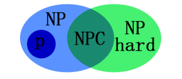
算法导论—SAT、NP、NPC、NP-Hard问题
算法导论—SAT、NP、NP-Hard、NPC问题SAT 问题基本定义问题复杂性P、NP、NP-Hard、NP-Complete(NPC)证明NP-Hard关系图NP问题的概念约化的定义NPC问题NP-Hard问题SAT 问题基本定义 SAT 问题 (Boolean satisfiability problem, 布尔可满足性问题,SAT): 给…...
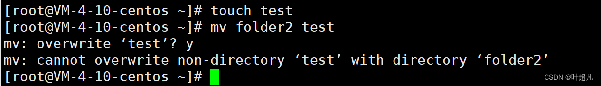
linux入门---基础指令(上)
这里写目录标题前言ls指令pwd指令cd指令touch指令mkdirrmdirrmman指令cp指令mv指令前言 我们平时使用电脑主要是通过鼠标键盘以及操作系统中自带的图形来对电脑执行相应的命令,比如说我想打开D盘中的cctalk这个文件: 我就可以先用鼠标左键单击这个文件…...
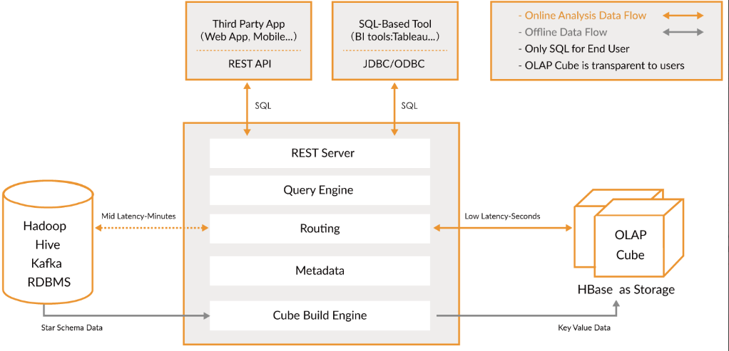
大数据Kylin(一):基础概念和Kylin简介
文章目录 基础概念和Kylin简介 一、OLTP与OLAP 1、OLTP 2、OLAP 3、OLTP与OLAP的关系 二、数据分析模型 1、星型模型 2、雪花模型 …...

推进行业生态发展完善,中国信通院第八批RPA评测工作正式启动
随着人工智能、云计算、大数据等新兴数字技术的高速发展,数字劳动力应用实践步伐加快,以数字生产力、数字创造力为基础的数字经济占比逐年上升。近年来,机器人流程自动化(Robotic Process Automation,RPA)成…...

DOM编程-获取下拉列表选中项的value
<!DOCTYPE html> <html> <head> <meta charset"utf-8"> <title>获取下拉列表选中项的value</title> </head> <body> <script type"text/javascript"> …...

认证服务-----技术点及亮点
大技术Nacos做注册中心把新建的微服务注册到Nacos上去两个步骤 在配置文件中配置应用名称、nacos的发现注册ip地址,端口号在启动类上用EnableDiscoveryClient注解开启注册功能使用Redis存验证码信息加入依赖配置地址和端口号即可直接注入StringRedisTemplate模板类用…...

6个常见的 PHP 安全性攻击
了解常见的PHP应用程序安全威胁,可以确保你的PHP应用程序不受攻击。因此,本文将列出 6个常见的 PHP 安全性攻击,欢迎大家来阅读和学习。 1、SQL注入 SQL注入是一种恶意攻击,用户利用在表单字段输入SQL语句的方式来影响正常的SQL执…...
三大基础排序算法——冒泡排序、选择排序、插入排序
目录前言一、排序简介二、冒泡排序三、选择排序四、插入排序五、对比References前言 在此之前,我们已经介绍了十大排序算法中的:归并排序、快速排序、堆排序(还不知道的小伙伴们可以参考我的 「数据结构与算法」 专栏)࿰…...
负载均衡上传webshell+apache换行解析漏洞
目录一、负载均衡反向代理下的webshell上传1、nginx负载均衡2、负载均衡下webshell上传的四大难点难点一:需要在每一台节点的相同位置上传相同内容的webshell难点二:无法预测下一次请求是哪一台机器去执行难点三:当我们需要上传一些工具时&am…...

【ESP 保姆级教程】玩转emqx数据集成篇③ ——消息重发布
忘记过去,超越自己 ❤️ 博客主页 单片机菜鸟哥,一个野生非专业硬件IOT爱好者 ❤️❤️ 本篇创建记录 2023-02-10 ❤️❤️ 本篇更新记录 2023-02-10 ❤️🎉 欢迎关注 🔎点赞 👍收藏 ⭐️留言📝🙏 此博客均由博主单独编写,不存在任何商业团队运营,如发现错误,请…...

动态紧凑模型在电子热设计中的高效应用
1. 动态紧凑模型在电子热设计中的核心价值在电子设备日益小型化、高功率化的今天,热管理已成为决定产品可靠性的关键因素。传统热仿真方法面临两大痛点:一是计算资源消耗大,特别是处理复杂封装结构时;二是难以准确预测半导体器件的…...

Claw Mentor:为OpenClaw智能体实现自动化配置同步与社区化演进
1. 项目概述:为你的AI智能体引入“导师”机制在AI智能体(Agent)开发领域,尤其是基于OpenClaw这类开源框架时,我们常常面临一个困境:如何持续地学习和迭代,跟上领域内最佳实践的发展速度…...

Flutter中如何显示异步数据
在开发Flutter应用时,处理异步操作是非常常见的任务之一。许多时候,我们需要将异步操作的结果展示在用户界面上,比如从服务器获取数据或执行一些耗时的计算。本文将通过一个具体的实例,展示如何在Flutter中使用FutureBuilder来处理和显示异步数据。 问题背景 假设我们有一…...

量子计算串扰问题与优化控制技术解析
1. 量子计算中的串扰问题与优化控制技术概述在量子计算硬件中,串扰(Crosstalk)是影响量子门操作精度的主要噪声源之一。当多个量子比特并行操作时,一个量子比特的控制脉冲会意外影响邻近量子比特的状态,这种现象在超导…...

编程应届生面试,HR最常问的20个问题,高分答案都在这里
文章目录前言一、自我认知类:HR想知道你是不是“对的人”问题1:请你做一个3分钟的自我介绍问题2:你最大的优点和缺点是什么?问题3:你为什么选择这个专业/行业?二、职业规划类:看你能不能在公司待…...

2026届毕业生推荐的六大AI辅助写作助手实际效果
Ai论文网站排名(开题报告、文献综述、降aigc率、降重综合对比) TOP1. 千笔AI TOP2. aipasspaper TOP3. 清北论文 TOP4. 豆包 TOP5. kimi TOP6. deepseek 在当下人工智能内容生成越来越普及的状况下,怎样去施行有效的“降AI”࿰…...

TikTok评论采集工具:如何轻松获取海量用户反馈数据?
TikTok评论采集工具:如何轻松获取海量用户反馈数据? 【免费下载链接】TikTokCommentScraper 项目地址: https://gitcode.com/gh_mirrors/ti/TikTokCommentScraper 在社交媒体分析领域,TikTok评论数据蕴含着丰富的用户洞察价值&#x…...

3步解锁Switch离线观影:揭秘wiliwili如何破解掌机视频播放四大难题
3步解锁Switch离线观影:揭秘wiliwili如何破解掌机视频播放四大难题 【免费下载链接】wiliwili 第三方B站客户端,目前可以运行在PC全平台、PSVita、PS4 、Xbox 和 Nintendo Switch上 项目地址: https://gitcode.com/GitHub_Trending/wi/wiliwili 你…...

OpenCore Legacy Patcher终极指南:五步让老Mac重获新生
OpenCore Legacy Patcher终极指南:五步让老Mac重获新生 【免费下载链接】OpenCore-Legacy-Patcher Experience macOS just like before 项目地址: https://gitcode.com/GitHub_Trending/op/OpenCore-Legacy-Patcher 你是否还在为手中的老旧Mac无法升级到最新…...

保姆级教程:在STM32CubeIDE项目中集成SEGGER RTT,并用J-Scope抓取波形
STM32CubeIDE实战:SEGGER RTT与J-Scope联调全攻略 在嵌入式开发中,实时观测变量变化是调试过程中不可或缺的一环。传统调试方法如串口打印或断点调试往往存在效率低下或干扰系统运行的问题。本文将手把手教你如何在STM32CubeIDE项目中集成SEGGER RTT技术…...