大模型参数高效微调PEFT的理解和应用
简介
近年的大型语言模型(也被称作基础模型),大多是采用大量资料数据和庞大模型参数训练的结果,比如常见的ChatGPT3有175B的模型参数量。随着Large Language Model(LLM)的横空出世,网络模型对常见问题的解答有了很强的泛化能力。但是如果将LLM应用到特定专业场景,如律师、医生,却仍表现的不尽如人意。即使可以使用few-shot learning或finetuning的技术进行迭代更新,但是模型参数的更新需要昂贵的机器费用。因此近年来,学术界大量研究人员开始从事高效Finetuning的工作,称作Effective Parameter Fine-Tuning(PEFT)。本次从方法构造的区别,可以将现有的PEFT方法分为Adapter、LoRA、Prefix Learning和Soft Prompt。学习过程很大程度上借鉴了李宏毅老师分享的2022 AACL-IJCNLP课件,有兴趣的读者可以翻阅原文链接。
方法
虽然LLM有很好的泛化能力,但如果需要应用到特定的场景任务,常常需要对LLM进行模型微调。问题是LLM的模型参数非常庞大,特定任务的微调需要昂贵的显卡资源,那么如何解决这样的问题呢?很显然,降低微调的模型参数量就是最简单的方法。试验表明,当每个特定任务微调时,只训练模型的一小部分参数,也能得到不错的效果。
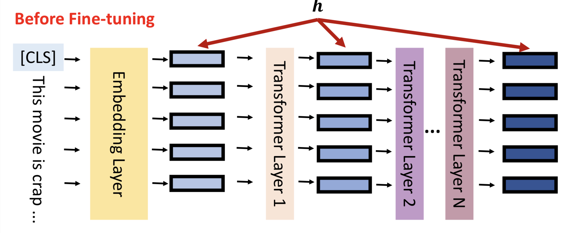
让我们回到模型微调的真实含义,如图所示,h表示每一层隐藏层的输出。

模型微调就是通过数据更新隐藏层的输出结果,更好的拟合输入数据的分布,对下游任务有更佳的表现,我们将隐藏层输出成为hidden representation(h)。
模型微调的结果就是更新hidden representation,用数学语言可以表示为:
h’ = h + 𝚫h
接下来介绍4种不同的方法,通过减少模型参数更新的数量,高效的更新𝚫h。
Adapter方法
Adapter方法通常是在网络模型中增加小型的模型块,通过冻结LLM的参数,仅更新Adapter模块的方式进行模型微调。

如图所示,Adapter应用在Transformer的结构中,在Multi-headed attention和Feed-forward网路层后紧接Adapter子模块,模型训练的时候冻结Transformer的参数,仅更新Adapter的参数。
LoRA方法
LoRA提出的想法是,既然LLM可以泛化用于不同的NLP任务,那么说明不同的任务有不同的神经元来处理,我们只要针对下游任务找到合适的那一批神经元,并对他们的权重进行强化,那么对下游任务也有显著的效果。

LoRA方法假设下游任务只需要低秩矩阵就可以找到大模型中对应的权重,然后仅更新小部分的模型参数,就可以在下游任务中表现不错。

如图所示,LoRA将𝚫h的计算方式更改为两个低秩矩阵的乘法,r表示矩阵秩的大小。那么模型的更新过程可以用数学方式表示为:
W= W + 𝚫W = W + BA, r << min(d_ffw, d_model)
Prefix Learning方法
Prefix Learning方法就是在网络层中,将网络层中扩展可训练的前缀。

这里以Self-Attention为例,先回忆一下Self-Attention的结构。
Self-Attention的数学表示为:
A t t e n t i o n ( Q , K , V ) = s o f t m a x ( Q K T d k V ) Attention(Q,K,V) = softmax(\frac{QK^T}{\sqrt{d_k}} V) Attention(Q,K,V)=softmax(dkQKTV)
首先初始化W_k, W_q, W_v参数,通过 q 1 = x 1 ∗ W q , k 1 = x 1 ∗ W k , v 1 = x 1 ∗ W v q_1=x_1*W_q, k_1=x_1* W_k, v_1=x_1 * W_v q1=x1∗Wq,k1=x1∗Wk,v1=x1∗Wv的方式得到QKV矩阵;
通过 α 1 , 1 = q 1 ∗ k 1 , α 1 , 2 = q 1 ∗ k 2 … \alpha1,1 = q_1 * k_1, \alpha1,2=q_1 * k_2… α1,1=q1∗k1,α1,2=q1∗k2… 的方式获取𝛼矩阵;
通过 z 1 , 1 = s o f t m a x ( α 1 , 1 ∗ v 1 ) … z1,1=softmax(\alpha1,1 * v1)… z1,1=softmax(α1,1∗v1)…的方式得到x1对其他token的注意力
最后累加计算得出 x 1 ′ x'_1 x1′的结果,如此循环计算下一个时刻输出。

PreFix Tuning的做法是对self-attention增加一部分参数,计算𝚫h的结果。
如图所示,增加了3个参数量,模型训练的时候只更新这3个用到的的参数。

Soft Prompt方法
Soft Prompt的做法比较简单,直接在Embedding输出,插入一部分Prefix embedding信息。

Soft Prompt的简化版本是直接在input sequence句首插入文本。

小结
了解4种PEFT的方法后,可以发现PEFT有非常多的好处。
首先,PEFT可以极大的降低finetune的参数量。

如图所示,Adapter训练参数之占模型的5%,LoRa、Prefix Tuning和Soft Prompt的训练参数甚至小于0.1%。
其次,由于训练参数的减少,PEFT更不容易造成模型的过拟合,某种意义也是一种Dropout方法。
最后,由于需要更新的参数少,基础模型在小数据集上有不错的表现。
实践
我们以最受欢迎的LoRA为例,搭建一个简易的demo理解如何使用LoRA微调模型。
Demo的有2个不同分布的数据,分别是均匀分布和高斯分布;然后构造3层的ReLU-MLP对均匀分布数据进行训练;最后通过LoRA的对高斯分布数据进行微调。
首先是构造数据,分别生成均匀分布和高斯分布的数据集,lable范围都是{-1,1}。
import numpy as np
import torch
import matplotlib.pyplot as plt
from torch.utils.data import TensorDataset, DataLoader
import random
from collections import OrderedDict
import math
import torch.nn.functional as F
random.seed(42)def generate_uniform_sphere(n, d):normal_data = np.random.normal(loc=0.0, scale=1.0, size=[n, d])lambdas = np.sqrt((normal_data * normal_data).sum(axis=1))data = np.sqrt(d) * normal_data / lambdas[:, np.newaxis]return data# data type could be "uniform" or "gaussian"
def data_generator(data_type='uniform', inp_dims=100, sample_size=10000):if data_type == 'uniform':data = generate_uniform_sphere(sample_size, inp_dims)elif data_type == 'gaussian':var = 1.0 / inp_dimsdata = np.random.normal(loc=0.0, scale=var, size=[sample_size, inp_dims])labels = np.sign(np.mean(data, -1))for i in range(sample_size):if labels[i] == 0:labels[i] = 1return data, labels
第二步,构造3层的MLP网络模型,ReLU作为激活函数。
class ReluNN(torch.nn.Module):def __init__(self, inp_dims, h_dims, out_dims=1):super(ReluNN, self).__init__()self.inp_dims = inp_dimsself.h_dims = h_dimsself.out_dims = out_dims# build modelself.layer1 = torch.nn.Linear(self.inp_dims, self.h_dims)self.layer2 = torch.nn.Linear(self.h_dims, self.h_dims)self.last_layer = torch.nn.Linear(self.h_dims, self.out_dims, bias=False)def forward(self, x: torch.Tensor) -> torch.Tensor:x = torch.flatten(x, start_dim=1)x = self.layer1(x)x = torch.nn.ReLU()(x)x = self.layer2(x)x = torch.nn.ReLU()(x)x = self.last_layer(x)return xdef calc_loss(logits, labels):return torch.mean(torch.log(1 + torch.exp(-1 * torch.mul(labels.float(), logits.T))))def evaluate(labels, loss=None, output=None, iter=0, training_time=True):correct_label_count = 0for i in range(len(output)):if (output[i] * labels[i] > 0).item():correct_label_count += 1if training_time:print('Iteration: ', iter, ' Loss: ', loss, ' Correct label: ', correct_label_count, '/', len(output))else:print('Correct label: ', correct_label_count, '/', len(output), ', Accuracy: ', correct_label_count / len(output))
第三步,开始训练均匀分布数据。
# input dimensions
inp_dims = 16
# hidden dimensions in our model
h_dims = 32
# training sample size
n_train = 2000
# starting learning rate (I didn't end up using any learning rate scheduler. So this will be constant. )
starting_lr = 1e-4
batch_size = 256# generate data and build pytorch data pipline using TensorDataset module
data_train, labels_train = data_generator(data_type="uniform", inp_dims=inp_dims, sample_size=n_train)
dataset = TensorDataset(torch.Tensor(data_train), torch.Tensor(labels_train))
loader = DataLoader(dataset, batch_size=batch_size, drop_last=True)# Build the model and define optimiser
model = ReluNN(inp_dims, h_dims)
optimizer = torch.optim.Adam(model.parameters(), lr=starting_lr)# ---------------------
# Training loop here
# ---------------------its = 0
epochs = 400
print_freq = 200for epoch in range(epochs):for batch_data, batch_labels in loader:optimizer.zero_grad()output = model(batch_data)loss = calc_loss(output, batch_labels)loss.backward()optimizer.step()if its % print_freq == 0:correct_labels = evaluate(labels=batch_labels, loss=loss.detach().numpy(), output=output, iter=its, training_time=True)its += 1
获取训练输出结果:
Iteration:  0  Loss:  0.6975772  Correct label:  126 / 256
Iteration:  200  Loss:  0.6508794  Correct label:  164 / 256
Iteration:  400  Loss:  0.52307904  Correct label:  215 / 256
Iteration:  600  Loss:  0.34722215  Correct label:  240 / 256
Iteration:  800  Loss:  0.21760023  Correct label:  251 / 256
Iteration:  1000  Loss:  0.19394015  Correct label:  241 / 256
Iteration:  1200  Loss:  0.124890685  Correct label:  250 / 256
Iteration:  1400  Loss:  0.10578571  Correct label:  250 / 256
Iteration:  1600  Loss:  0.07651  Correct label:  252 / 256
Iteration:  1800  Loss:  0.05156578  Correct label:  256 / 256
Iteration:  2000  Loss:  0.045886587  Correct label:  256 / 256
Iteration:  2200  Loss:  0.04692286  Correct label:  256 / 256
Iteration:  2400  Loss:  0.06285152  Correct label:  254 / 256
Iteration:  2600  Loss:  0.03973126  Correct label:  254 / 256
在均匀分布和高斯分布测试集分别进行测试:
print('-------------------------------------------------')
print('Test model performance on uniformly-distributed data (the data we trained our model on)')
data_test, labels_test = data_generator(data_type="uniform", inp_dims=inp_dims, sample_size=1024)
data_test = torch.Tensor(data_test)
labels_test = torch.Tensor(labels_test)output = model(data_test)
correct_labels = evaluate(labels=labels_test, loss=0.0, output=output, iter=0, training_time=False)print('-------------------------------------------------')
print('Test model performance on normally-distributed data')
data_test, labels_test = data_generator(data_type="gaussian", inp_dims=inp_dims, sample_size=1024)
data_test = torch.Tensor(data_test)
labels_test = torch.Tensor(labels_test)output = model(data_test)
correct_labels = evaluate(labels=labels_test, loss=0.0, output=output, iter=0, training_time=False)
print('-------------------------------------------------')
获得输出结果为,均匀分布表现远高于高斯分布,这是理所当然的。
-------------------------------------------------
Test model performance on uniformly-distributed data (the data we trained our model on)
Correct label:   1007 / 1024 , Accuracy:  0.9833984375
-------------------------------------------------
Test model performance on normally-distributed data
Correct label:   832 / 1024 , Accuracy:  0.8125
-------------------------------------------------
第四步,实现LoRA改造网络模型,LoRA代码实现来自https://github.com/microsoft/LoRA/tree/main。
class LoRALinear(torch.nn.Linear):def __init__(self, layer: torch.nn.Linear, r: int, lora_alpha: float, in_features: int, out_features: int,**kwargs, ):torch.nn.Linear.__init__(self, in_features, out_features, **kwargs)# trainable parametersself.weight = layer.weightself.r = rif self.r > 0:# lora_A matrix has shape [number of ranks, number of input features]self.lora_A = torch.nn.Parameter(self.weight.new_zeros((in_features, r)))# lora_A matrix has shape [number of output features, number of ranks]self.lora_B = torch.nn.Parameter(self.weight.new_zeros((r, out_features)))self.scaling = lora_alpha / r# Freezing the pre-trained weight matrixself.weight.requires_grad = Falseself.reset_parameters()def reset_parameters(self):if hasattr(self, 'lora_A'):torch.nn.init.kaiming_uniform_(self.lora_A, a=math.sqrt(5))torch.nn.init.zeros_(self.lora_B)def forward(self, x: torch.Tensor):if self.r > 0:result = F.linear(x, self.weight, bias=self.bias) result += (x @ self.lora_A @ self.lora_B) * self.scalingreturn resultelse:return F.linear(x, self.weight, bias=self.bias)
改造第二层网络层:
ranks = 2
l_alpha = 1.0# wrap the second layer of the model
lora_layer2 = LoRALinear(model.layer2, r=ranks, lora_alpha=l_alpha, in_features=h_dims, out_features=h_dims)
开始进行微调训练:
# new pipline that contains data generated from Gaussian distribution
ft_data_train, ft_labels_train = data_generator(data_type="gaussian", inp_dims=inp_dims, sample_size=n_train)
ft_data_test, ft_labels_test = data_generator(data_type="gaussian", inp_dims=inp_dims, sample_size=n_train)
dataset = TensorDataset(torch.Tensor(ft_data_train), torch.Tensor(ft_labels_train))
ft_loader = DataLoader(dataset, batch_size=batch_size, drop_last=False)# Adam now takes the 160 trainable LoRA parameters
starting_lr = 1e-3
optimizer = torch.optim.Adam(lora_layer2.parameters(), lr=starting_lr)# ---------------------
# Training starts again
# ---------------------its = 0
epochs = 400
print_freq = 200for epoch in range(epochs):for batch_data, batch_labels in ft_loader:optimizer.zero_grad()x = model.layer1(batch_data)x = torch.nn.ReLU()(x)# ---this is the new layer---x = lora_layer2(x)# ---------------------------x = torch.nn.ReLU()(x)output = model.last_layer(x)loss = calc_loss(output, batch_labels)loss.backward()optimizer.step()if its % print_freq == 0:correct_labels = evaluate(labels=batch_labels, loss=loss.detach().numpy(), output=output, iter=its, training_time=True)its += 1
微调输出结果为:
Iteration:  0  Loss:  0.41668275  Correct label:  194 / 256
Iteration:  200  Loss:  0.34483075  Correct label:  249 / 256
Iteration:  400  Loss:  0.28130627  Correct label:  247 / 256
Iteration:  600  Loss:  0.18952605  Correct label:  249 / 256
Iteration:  800  Loss:  0.14345655  Correct label:  249 / 256
Iteration:  1000  Loss:  0.117519796  Correct label:  250 / 256
Iteration:  1200  Loss:  0.100797206  Correct label:  251 / 256
Iteration:  1400  Loss:  0.08887711  Correct label:  252 / 256
Iteration:  1600  Loss:  0.07975915  Correct label:  253 / 256
Iteration:  1800  Loss:  0.07250729  Correct label:  253 / 256
Iteration:  2000  Loss:  0.06658038  Correct label:  253 / 256
Iteration:  2200  Loss:  0.061622016  Correct label:  254 / 256
Iteration:  2400  Loss:  0.057407677  Correct label:  254 / 256
Iteration:  2600  Loss:  0.05379172  Correct label:  254 / 256
Iteration:  2800  Loss:  0.050651148  Correct label:  254 / 256
Iteration:  3000  Loss:  0.04789203  Correct label:  255 / 256
最后一步,再次测试高斯分布的数据集。
data_test, labels_test = data_generator(data_type="gaussian", inp_dims=inp_dims, sample_size=1024)
data_test = torch.Tensor(data_test)
labels_test = torch.Tensor(labels_test)x = model.layer1(data_test)
x = torch.nn.ReLU()(x)
# ---this is the new layer---
x = lora_layer2(x)
# ---------------------------
x = torch.nn.ReLU()(x)
output = model.last_layer(x)
correct_labels = evaluate(labels=labels_test, loss=0.0, output=output, iter=0, training_time=False)
输出结果为:
Correct label: 1011 / 1024 , Accuracy: 0.9873046875
微调效果很明显,准确率从81.2%提升到98.7%。最后再计算LoRA微调的参数量大小。
def count_parameters(model):return sum(p.numel() for p in model.parameters() if p.requires_grad)print("Original second layer parameters: ", count_parameters(original_layer2))
print("LoRA layer parameters: ", count_parameters(lora_layer2))
输出结果为:
Original second layer parameters:  1056
LoRA layer parameters:  160
通过实验结果发现,原始模型参数量1056,LoRA参数量160,仅为原来的1/10,但是训练效果从81.2%提升到98.7%。
总结
如果对网络层每一层都要重新实现LoRA的方法,是比较复杂的,推荐使用HuggingFace的封装库peft,覆盖基本的网络模型。
- 共用基础LLM是未来的趋势,如果需要快速适应特殊的任务,只需要训练LoRA的参数即可,大大降低了GPU的使用量;
- 当不同任务的切换时,只需要切换不同的LoRA参数;
参考
- Houlsby, Neil, et al. “Parameter-efficient transfer learning for NLP.” International Conference on Machine Learning. PMLR, 2019.
- Hu, Edward J., et al. “LoRA: Low-Rank Adaptation of Large Language Models.” International Conference on Learning Representations. 2021.
- The Power of Scale for Parameter-Efficient Prompt Tuning. Proceedings of the 2021 Conference on Empirical Methods in Natural Language Processing. 2021
相关文章:
大模型参数高效微调PEFT的理解和应用
简介 近年的大型语言模型(也被称作基础模型),大多是采用大量资料数据和庞大模型参数训练的结果,比如常见的ChatGPT3有175B的模型参数量。随着Large Language Model(LLM)的横空出世,网络模型对常见问题的解答有了很强的…...

工作游戏时mfc140u.dll丢失的解决方法,哪个方法可快速修复mfc140u.dll问题
在 Windows 操作系统中,mfc140u.dll 文件是非常重要的一个组件,许多基于 MFC(Microsoft Foundation Classes)的程序都需要依赖这个文件。然而,有些用户在运行这些程序时可能会遇到mfc140u.dll丢失的问题,导…...
选择排序——直接选择排序
直接选择排序:(以重复选择的思想为基础进行排序) 1、简述 顾名思义就是选出一个数,再去抉择放哪里去。 设记录R1,R2…,Rn,对i1,2,…,n-1,重复下…...
【C++基础】观察者模式(“发布-订阅”模式)
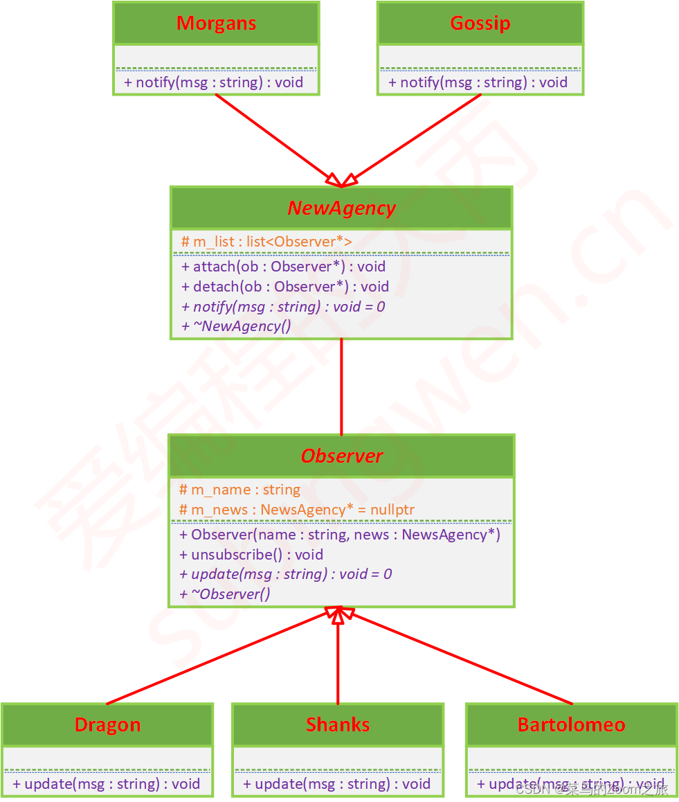
本文参考:观察者模式 - 摩根斯 | 爱编程的大丙 观察者模式允许我们定义一种订阅机制,可在对象事件发生时通知所有的观察者对象,使它们能够自动更新。观察者模式还有另外一个名字叫做“发布-订阅”模式。 发布者: 添加订阅者&…...
从业多年,我总结出软件测试工程师必须掌握的技能,你不可错过!
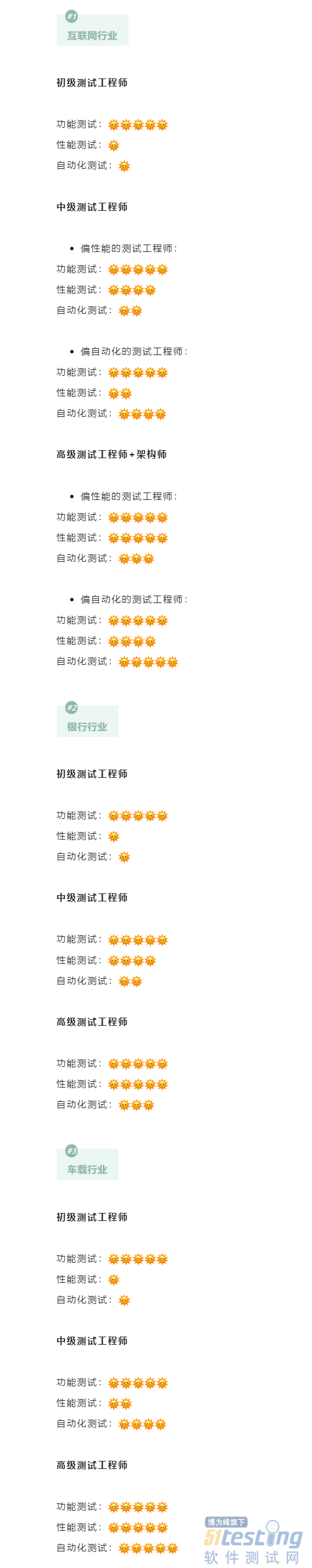
经常会有小伙伴询问:“测试工程师有哪些必须要掌握的技能?”这是一个非常大的课题,因为每个人从事的行业不同、岗位不同,需要掌握的技能自然也不一样。 今天小编就从不同岗位、不同行业两个大方面,来讲讲软件测试工程师…...

【nerfStudio】5-nerfStudio导出3D Mesh模型
几何图形的导出 在这里我们将介绍如何从nerfstudio中导出点云和网格。您将使用的主要命令是ns-export。我们将点云导出为.ply文件,纹理网格导出为.obj文件。 导出网格 1. TSDF融合 TSDF(截断有符号距离函数)融合是一种使用深度图像提取表面网格的算法。此方法适用于所有…...

重要公告|投票委托已经上线,应该如何选择社区代表?
社区代表是Token持有者委托投票权的个人或团体,可以代表Token持有者在Moonbeam治理中投票。委托是可选的,允许代表在治理过程中代表更大比例的Token和Token持有者。相比社区代表,不愿投票的Token持有者可以将投票权委托给社区代表,…...
【操作系统】聊聊进程、线程、协程
进程内部有那些数据 为什么创建进程的成本高 进程和线程 进程是资源分配的基本单位,而线程是程序执行的基本单位,一个是从资源分配的角度看,另一个是执行角度。 那么进程和程序的区别是什么? 程序,一段代码ÿ…...

springboot 下 activiti 7会签配置与实现
流程图配置 会签实现须在 userTask 节点下的 multi instance 中配置 collection 及 completion condition; collection 会签人员列表;element variable 当前会签变量名称,类似循环中的 item;completion condition: 完成条件。 ${taskExecutionServiceIm…...

RK3399平台开发系列讲解(内核调试篇)spidev_test工具使用
🚀返回专栏总目录 文章目录 一、环境二、执行测试三、回环测试四、字节发送测试五、32位数据发送测试沉淀、分享、成长,让自己和他人都能有所收获!😄 📢 在 Linux 系统上,“spidev_test” 是一个用于测试和配置 SPI(Serial Peripheral Interface)设备的命令行工具。…...
)
点云从入门到精通技术详解100篇-自适应点云局部邻域特征的特征提取与配准(续)
目录 3.4 深度相机误差建模 3.5 实验结果及分析 3.5.1 TOF 相机平面畸变校正 3.5.2 TOF 相机深度误差校正...

VBA技术资料MF52:VBA_在Excel中突出显示前 10 个值
【分享成果,随喜正能量】一言之善,重于千金。善良不分大小,有时候你以为的一句话,小小的举手之劳,也可能就是别人的救赎!不要吝啬你的善良,因为你永远不知道那小小的善良能给多少人带来光明。。…...

leetcode做题笔记134. 加油站
在一条环路上有 n 个加油站,其中第 i 个加油站有汽油 gas[i] 升。 你有一辆油箱容量无限的的汽车,从第 i 个加油站开往第 i1 个加油站需要消耗汽油 cost[i] 升。你从其中的一个加油站出发,开始时油箱为空。 给定两个整数数组 gas 和 cost &…...
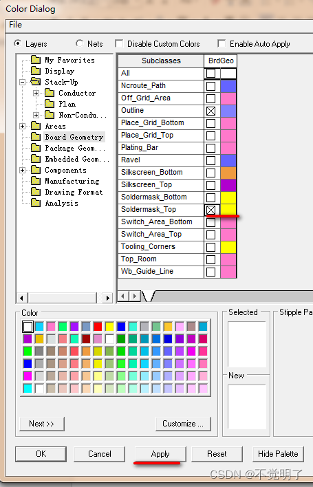
Allegro166版本如何在颜色管理器中实时显示层面操作指导
Allegro166版本如何在颜色管理器中实时显示层面操作指导 在用Allegro166进行PCB设计的时候,需要在颜色管理器中频繁的开关层面。但是166不像172一样在颜色管理器中可以实时的开关层面,如下图 需要打开Board Geometry/Soldermask_top层,首先需要勾选这个层面,再点击Apply即…...

纷享销客入选中国信通院《高质量数字化转型产品及服务全景图》
近期,在中国信息通信研究院主办的“2023数字生态发展大会”暨中国信通院“铸基计划”年中上,重磅发布了《高质量数字化转型产品及服务全景图(2023)》,纷享销客凭借先进的技术能力和十余年客户业务场景应用理解…...

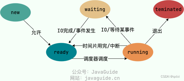
C高级 DAY4
一、分支语句 case ...in语句 shell中的switch语句 case $变量名 in常量1)语句;; ------->类似于C中break的作用,;;除了最后一条分之外,都不能省略常量2)语句;; 常量n)语句;;*) ------->类似于C中default,但…...
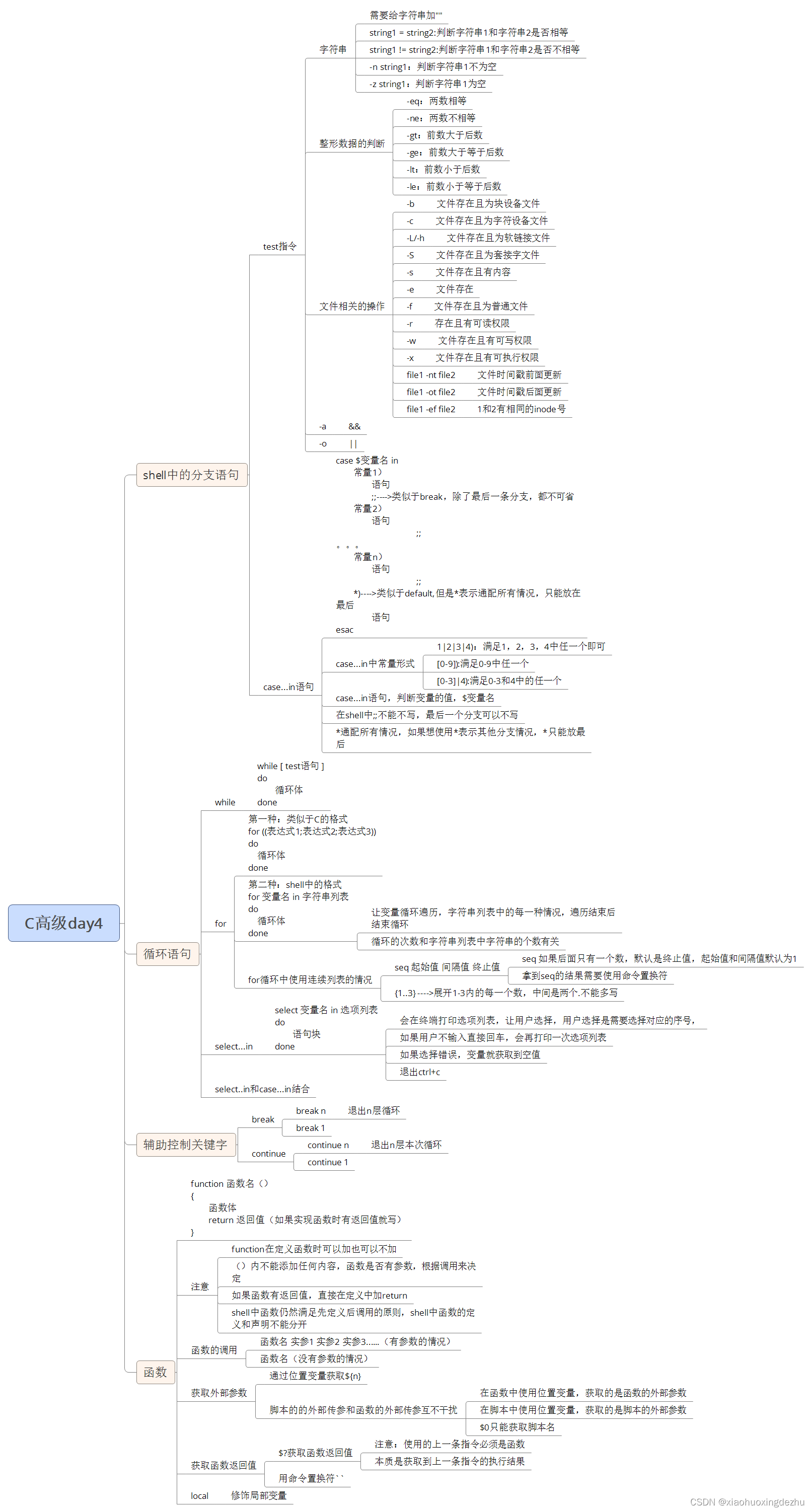
C高级day4
作业 实现一个对数组求和的函数,数组通过实参传递给函数 写一个函数,输出当前用户的uid和gid,并使用变量接收结果 思维导图...
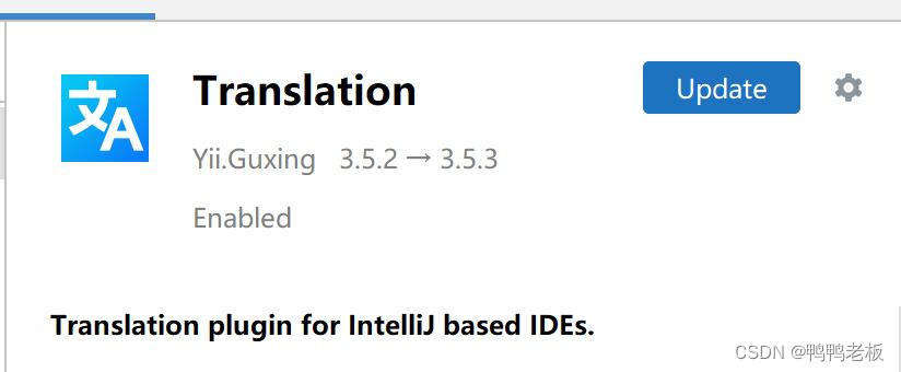
Java8-17 --- idea2022
目录 一、idea官网 二、使用idea编写hello world 三、查看工程中的JDK配置信息 四、详细设置 4.1、显示工具栏 4.2、默认启动项目配置 4.3、取消自动更新 4.4、选择整体主体与背景图 4.5、设置编辑器主题样式 4.5.1、编辑器主题 4.5.2、字体大小 4.5.3、修改注…...

Mybatis---增删改查
目录 一、添加用户 (1)持久层接口方法 (2)映射文件 (3)测试方法 二、修改用户 (1)持久层接口方法 (2)映射文件 (3)测试方法 …...
开机性能-如何抓取开机systrace
一、理论 1.背景 抓取开机 trace 需要使用 userdebug 版本,而我们测试开机性能问题时都要求使用 user 版本,否则会有性能损耗问题。因此想要在抓取开机性能trace 时,需要在 user 版本上打开 atrace 功能之后才能抓取 trace,默认 …...

Anaconda 安装与配置 的所有核心步骤
下载:去官网或靠谱的镜像源(如清华镜像)下载 2025.06版 Windows x64 安装包(约950MB)。安装:运行 .exe 文件。关键选项1:勾选 Add Anaconda to my PATH (添加到环境变量)…...

GP8892SEH贴片SOP7省外围5V2A隔离型原边反馈芯片直接替代MT3723
GP8892SEH 是一款自供电原边反馈 PWM 控制芯片,采用 SOP7 贴片封装,主打"省外围、高精度、低待机"路线。它内置功率三极管,无需外置功率管,同时集成了 FB 下偏电阻和 CS 采样电阻,外围元件极少,特…...

国产替代之NVMFS5C673NWFT1G 与 VBQA1615 参数对比报告
N沟道功率MOSFET参数对比分析报告一、产品概述NVMFS5C673NWFT1G:安森美(onsemi)N沟道功率MOSFET,耐压60V,极低导通电阻(10.7mΩ),采用先进沟槽工艺,具有低栅极电荷和电容…...

别再瞎写 Prompt 了:2026年最实用的10条LLM提示词技巧
别再瞎写 Prompt 了:2026年最实用的10条LLM提示词技巧强烈推荐收藏!从 OpenAI 官方指南到社区实践精华,每条技巧都附带 ❌ 错误示范 → ✅ 正确示范 → 💡 原理说明。这个问题你肯定遇到过 你打开 ChatGPT,输入&#x…...

HUM4D数据集:无标记人体动作捕捉的挑战与评估
1. HUM4D数据集概述HUM4D是一个专门针对无标记人体动作捕捉技术评估的基准数据集,由计算机视觉研究团队开发。这个数据集的核心价值在于填补了现有动作捕捉基准在复杂场景下的空白——那些包含快速运动、严重遮挡、深度突变和身份混淆的真实挑战。在动作捕捉领域&am…...

为LibraVDB定制内存池:提升稀疏体素数据处理性能
1. 项目概述:一个为LibraVDB设计的开源内存管理库最近在搞一些基于体素的数据处理项目,特别是用到了LibraVDB这个开源的稀疏体素数据库。玩过VDB格式的朋友都知道,它的核心优势在于对稀疏体数据的极致压缩和高效访问,但这也带来了…...

技能图谱探索器:从数据建模到交互可视化的全栈实现
1. 项目概述:一个技能图谱的探索工具最近在GitHub上看到一个挺有意思的项目,叫nitzzzu/openclaw-skills-explorer。光看名字,openclaw和skills-explorer这两个词就挺有画面感的。我第一反应是,这应该是一个用来探索、梳理或可视化…...

VSCode + Cline + Codeium + OpenSpec + DeepSeek 完整配置指南
VSCode Cline Codeium OpenSpec DeepSeek 完整配置指南 📋 最终方案概述 组件用途费用VSCode代码编辑器免费Codeium (Windsurf)Tab 补全 生成注释免费ClineAI Agent(复杂任务、多文件操作)免费OpenSpec规范驱动开发(复杂功…...

5分钟快速上手:如何用Video2X免费AI工具让老旧视频焕发4K新生
5分钟快速上手:如何用Video2X免费AI工具让老旧视频焕发4K新生 【免费下载链接】video2x A machine learning-based video super resolution and frame interpolation framework. Est. Hack the Valley II, 2018. 项目地址: https://gitcode.com/GitHub_Trending/v…...
)
Google Maps路线响应延迟超800ms?Gemini边缘推理加速方案上线即降为112ms(附可复用TensorRT优化脚本)
更多请点击: https://intelliparadigm.com 第一章:Gemini Google Maps路线优化 Google Maps 与 Gemini 的深度集成正在重塑企业级物流与出行服务的智能边界。通过 Gemini 的多模态推理能力,开发者可将自然语言查询(如“避开施工路…...