跟着Nature Communications学作图:纹理柱状图+添加显著性标签!
📋文章目录
- 复现图片
- 设置工作路径和加载相关R包
- 读取数据集
- 数据可视化
- 计算均值和标准差
- 方差分析
- 组间t-test
- 图a可视化过程
- 图b可视化过程
- 合并图ab
跟着「Nature Communications」学作图,今天主要通过复刻NC文章中的一张主图来巩固先前分享过的知识点,比如纹理柱状图、 添加显著性标签、拼图等,其中还会涉及数据处理的相关细节和具体过程。
复现图片


主要复现红框部分,右侧的cd图与框中的图是同类型的,只不过需要构建更多数据相对麻烦,所以选择以左侧红框图进行学习和展示。
设置工作路径和加载相关R包
rm(list = ls()) # 清空当前环境变量
setwd("C:/Users/Zz/Desktop/公众号 SES") # 设置工作路径
# 加载R包
library(ggplot2)
library(agricolae)
library(ggpattern)
library(ggpubr)
读取数据集
cData1 <- read.csv("cData1.csv", header = T, row.names = 1)
head(cData1)
#   Type   Deep ctValue ftValue Stripe_Angle
# 1   BT    Top      55      73          135
# 2   BT    Top      61      78          135
# 3   BT    Top      69      80          135
# 4   BT Center      35      50          135
# 5   BT Center      42      41          135
# 6   BT Center      43      57          135
数据包括以下指标:2个分类变量、2个数值变量、和1个整数变量。
数据可视化
在可视化前,我们需要先思考图中构成的元素,由哪些组成。
- 计算每个分组或处理下的均值和标准差;
- 进行组内的方差分析及多重比较;
- 进行组间的t检验;
计算均值和标准差
cData1_mean <- cData1 %>% gather(key = "var_type", value = "value",3:4) %>% group_by(Type, Deep, var_type, Stripe_Angle) %>%  summarise(mean = mean(value),sd = sd(value))
cData1_mean
# A tibble: 12 × 6
# Groups:   Type, Deep, var_type [12]
# Type  Deep   var_type Stripe_Angle  mean    sd
# <fct> <chr>  <chr>           <int> <dbl> <dbl>
# 1 BT    Bottom ctValue           135  47.7  1.53
# 2 BT    Bottom ftValue           135  48    1
# 3 BT    Center ctValue           135  40    4.36
# 4 BT    Center ftValue           135  49.3  8.02
# 5 BT    Top    ctValue           135  61.7  7.02
# 6 BT    Top    ftValue           135  77    3.61
# 7 CK    Bottom ctValue           135  42    7.21
# 8 CK    Bottom ftValue           135  48    4.36
# 9 CK    Center ctValue           135  38.3  2.08
# 10 CK    Center ftValue           135  47.7  5.13
# 11 CK    Top    ctValue           135  46.7  7.57
# 12 CK    Top    ftValue           135  53.7 12.3
方差分析
# 方差分析
groups <- NULL
vl <- unique((cData1 %>% gather(key = "var_type", value = "value", 3:4) %>% unite("unique_col", c(Type, var_type), sep = "-"))$unique_col)
vlfor(i in 1:length(vl)){df <- cData1 %>% gather(key = "var_type", value = "value", 3:4) %>% unite("unique_col", c(Type, var_type), sep = "-") %>% filter(unique_col == vl[i])aov <- aov(value ~ Deep, df)lsd <- LSD.test(aov, "Deep", p.adj = "bonferroni") %>%.$groups %>% mutate(Deep = rownames(.),unique_col = vl[i]) %>%dplyr::select(-value) %>% as.data.frame()groups <- rbind(groups, lsd)
}
groups <- groups %>% separate(unique_col, c("Type", "var_type"))
groups
#         groups   Deep Type var_type
# Top          a    Top   BT  ctValue
# Bottom       b Bottom   BT  ctValue
# Center       b Center   BT  ctValue
# Top1         a    Top   CK  ctValue
# Bottom1      a Bottom   CK  ctValue
# Center1      a Center   CK  ctValue
# Top2         a    Top   BT  ftValue
# Center2      b Center   BT  ftValue
# Bottom2      b Bottom   BT  ftValue
# Top3         a    Top   CK  ftValue
# Bottom3      a Bottom   CK  ftValue
# Center3      a Center   CK  ftValue
使用aov函数和LSD.test函数实现方差分析及对应的多重比较,并提取显著性字母标签。
然后将多重比较的结果与原均值标准差的数据进行合并:
cData1_mean1 <- left_join(cData1_mean, groups, by = c("Deep", "Type", "var_type")) %>% arrange(var_type) %>% group_by(Type, var_type) %>% mutate(label_to_show = n_distinct(groups))
cData1_mean1
# A tibble: 12 × 8
# Groups:   Type, var_type [4]
# Type  Deep   var_type Stripe_Angle  mean    sd groups label_to_show
# <chr> <chr>  <chr>           <int> <dbl> <dbl> <chr>          <int>
# 1 BT    Bottom ctValue           135  47.7  1.53 b                  2
# 2 BT    Center ctValue           135  40    4.36 b                  2
# 3 BT    Top    ctValue           135  61.7  7.02 a                  2
# 4 CK    Bottom ctValue           135  42    7.21 a                  1
# 5 CK    Center ctValue           135  38.3  2.08 a                  1
# 6 CK    Top    ctValue           135  46.7  7.57 a                  1
# 7 BT    Bottom ftValue           135  48    1    b                  2
# 8 BT    Center ftValue           135  49.3  8.02 b                  2
# 9 BT    Top    ftValue           135  77    3.61 a                  2
# 10 CK    Bottom ftValue           135  48    4.36 a                  1
# 11 CK    Center ftValue           135  47.7  5.13 a                  1
# 12 CK    Top    ftValue           135  53.7 12.3  a                  1
- 需要注意的是:这里添加了label_to_show一列,目的是为了后续再进行字母标签添加时可以识别没有显著性的结果。
组间t-test
cData1_summary <- cData1 %>%gather(key = "var_type", value = "value", 3:4) %>% # unite("unique_col", c(Type, Deep), sep = "-") %>% unique_colgroup_by(Deep, var_type) %>%summarize(p_value = round(t.test(value ~ Type)$p.value, 2)) %>%mutate(label = ifelse(p_value <= 0.001, "***",ifelse(p_value <= 0.01, "**", ifelse(p_value <= 0.05, "*", ifelse(p_value <= 0.1, "●", NA)))))
cData1_summary
# Deep   var_type p_value label
# <chr>  <chr>      <dbl> <chr>
# 1 Bottom ctValue     0.31 NA
# 2 Bottom ftValue     1    NA
# 3 Center ctValue     0.59 NA
# 4 Center ftValue     0.78 NA
# 5 Top    ctValue     0.07 ●
# 6 Top    ftValue     0.07 ●
我们将计算出来的p值,并用* 或者 ●进行了赋值。然后合并相关结果:
cData1_summary1 <- left_join(cData1_mean1, cData1_summary, by = c("Deep", "var_type"))
cData1_summary1
# Type  Deep   var_type Stripe_Angle  mean    sd groups label_to_show p_value label
# <chr> <chr>  <chr>           <int> <dbl> <dbl> <chr>          <int>   <dbl> <chr>
# 1 BT    Bottom ctValue           135  47.7  1.53 b                  2    0.31 NA
# 2 BT    Center ctValue           135  40    4.36 b                  2    0.59 NA
# 3 BT    Top    ctValue           135  61.7  7.02 a                  2    0.07 ●
# 4 CK    Bottom ctValue           135  42    7.21 a                  1    0.31 NA
# 5 CK    Center ctValue           135  38.3  2.08 a                  1    0.59 NA
# 6 CK    Top    ctValue           135  46.7  7.57 a                  1    0.07 ●
# 7 BT    Bottom ftValue           135  48    1    b                  2    1    NA
# 8 BT    Center ftValue           135  49.3  8.02 b                  2    0.78 NA
# 9 BT    Top    ftValue           135  77    3.61 a                  2    0.07 ●
# 10 CK    Bottom ftValue           135  48    4.36 a                  1    1    NA
# 11 CK    Center ftValue           135  47.7  5.13 a                  1    0.78 NA
# 12 CK    Top    ftValue           135  53.7 12.3  a                  1    0.07 ●
- 需要注意的是:添加的label也是为了后续筛选掉没有显著性结果做准备。
图a可视化过程
ctValue <- ggplot(data = cData1_mean1 %>% filter(var_type == "ctValue") %>% mutate(Deep = factor(Deep, levels = c("Top", "Center", "Bottom"))), aes(x = Type, y = mean, fill = Deep, pattern = Type, width = 0.75)) +geom_bar_pattern(position = position_dodge(preserve = "single"),stat = "identity",pattern_fill = "white", pattern_color = "white", pattern_angle = -50,pattern_spacing = 0.05,color = "grey",width = 0.75) +scale_pattern_manual(values = c(CK = "stripe", BT = "none")) +geom_errorbar(data = cData1_mean %>% filter(var_type == "ctValue") %>% mutate(Deep = factor(Deep, levels = c("Top", "Center", "Bottom"))), aes(x = Type, y = mean, ymin = mean - sd, ymax = mean + sd, width = 0.2),position = position_dodge(0.75),)+geom_point(data = cData1 %>% mutate(Deep = factor(Deep, levels = c("Top", "Center", "Bottom"))),aes(x = Type, y = ctValue, group = Deep), color = "black", fill = "#D2D2D2", shape = 21,position = position_dodge(0.75), size = 3)+geom_text(data = cData1_mean1 %>% filter(var_type == "ctValue",label_to_show > 1) %>% mutate(Deep = factor(Deep, levels = c("Top", "Center", "Bottom"))),aes(x = Type, y = mean + sd, label = groups), position = position_dodge(0.75), vjust = -0.5, size = 5) +geom_segment(data = cData1_summary1 %>% filter(p_value <= 0.1 & var_type == "ctValue"),aes(x = 0.75, xend = 0.75, y = 73, yend = 76))+geom_segment(data = cData1_summary1 %>% filter(p_value <= 0.1 & var_type == "ctValue"),aes(x = 0.75, xend = 1.75, y = 76, yend = 76))+geom_segment(data = cData1_summary1 %>% filter(p_value <= 0.1 & var_type == "ctValue"),aes(x = 1.75, xend = 1.75, y = 73, yend = 76))+geom_text(data = cData1_summary1 %>% filter(p_value <= 0.1 & var_type == "ctValue"),aes(x = 1.25, y = 76, label = paste0("p = ", p_value)),vjust = -0.5, size = 5)+geom_text(data = cData1_summary1 %>% filter(p_value <= 0.1 & var_type == "ctValue"),aes(x = 1.25, y = 78, label = label),vjust = -1, size = 5)+scale_fill_manual(values = c("#393939", "#A2A2A2", "#CCCCCC")) +scale_y_continuous(expand = c(0, 0), limits = c(0, 100), breaks = seq(0, 100, 50)) +theme_classic()+theme(legend.position = "top",axis.ticks.length.y = unit(0.2, "cm"),axis.text.y = element_text(color = "black", size = 12),axis.title.y = element_text(color = "black", size = 12, face = "bold"),axis.title.x = element_blank(),axis.text.x = element_blank(),axis.line.x = element_blank(),axis.ticks.x = element_blank(),plot.margin = margin(t = 0, r = 0, b = 1, l = 0, "lines"))+labs(y = "CTvalue", fill = "", pattern = "");ctValue

图b可视化过程
ftValue <- ggplot(data = cData1_mean1 %>% filter(var_type == "ftValue") %>% mutate(Deep = factor(Deep, levels = c("Top", "Center", "Bottom"))), aes(x = Type, y = mean, fill = Deep, pattern = Type, width = 0.75)
) +geom_bar_pattern(position = position_dodge(preserve = "single"),stat = "identity",pattern_fill = "white", pattern_color = "white", pattern_angle = -50,pattern_spacing = 0.05,color = "grey",width = 0.75) +scale_pattern_manual(values = c(CK = "stripe", BT = "none")) +geom_errorbar(data = cData1_mean %>% filter(var_type == "ftValue") %>% mutate(Deep = factor(Deep, levels = c("Top", "Center", "Bottom"))), aes(x = Type, y = mean, ymin = mean - sd, ymax = mean + sd, width = 0.2),position = position_dodge(0.75),)+geom_point(data = cData1 %>% mutate(Deep = factor(Deep, levels = c("Top", "Center", "Bottom"))),aes(x = Type, y = ftValue, group = Deep), color = "black", fill = "#D2D2D2", shape = 21,position = position_dodge(0.75), size = 3)+geom_text(data = cData1_mean1 %>% filter(var_type == "ftValue",label_to_show > 1) %>% mutate(Deep = factor(Deep, levels = c("Top", "Center", "Bottom"))),aes(x = Type, y = mean + sd, label = groups), position = position_dodge(0.75), vjust = -0.5, size = 5) +geom_segment(data = cData1_summary1 %>% filter(p_value <= 0.1 & var_type == "ftValue"),aes(x = 0.75, xend = 0.75, y = 85, yend = 88))+geom_segment(data = cData1_summary1 %>% filter(p_value <= 0.1 & var_type == "ftValue"),aes(x = 0.75, xend = 1.75, y = 88, yend = 88))+geom_segment(data = cData1_summary1 %>% filter(p_value <= 0.1 & var_type == "ftValue"),aes(x = 1.75, xend = 1.75, y = 85, yend = 88))+geom_text(data = cData1_summary1 %>% filter(p_value <= 0.1 & var_type == "ftValue"),aes(x = 1.25, y = 88, label = paste0("p = ", p_value)),vjust = -0.5, size = 5)+geom_text(data = cData1_summary1 %>% filter(p_value <= 0.1 & var_type == "ftValue"),aes(x = 1.25, y = 90, label = label),vjust = -1, size = 5)+scale_fill_manual(values = c("#393939", "#A2A2A2", "#CCCCCC")) +scale_y_continuous(expand = c(0, 0), limits = c(0, 100), breaks = seq(0, 100, 50)) +theme_classic()+theme(legend.position = "top",axis.ticks.length.y = unit(0.2, "cm"),axis.text.y = element_text(color = "black", size = 12),axis.title.y = element_text(color = "black", size = 12, face = "bold"),axis.title.x = element_blank(),axis.text.x = element_blank(),axis.line.x = element_blank(),axis.ticks.x = element_blank())+labs(y = "FTvalue", fill = "", pattern = "");ftValue

合并图ab
ggarrange(ctValue, ftValue, nrow = 2, ncol = 1, labels = c ("A", "B"),align = "hv", common.legend = T)

使用ggpubr包中的ggarrange函数完成拼图。
这个图展示了基于不同深度(Top、Center、Bottom)和类型(CK、BT)的ctValue。以下是一个简短的解读:
柱状图:使用geom_bar_pattern函数创建柱状图。柱子的高度代表每种类型和深度的平均ctValue。柱子的颜色是根据深度填充的,而模式则是基于类型填充的。
误差条:使用geom_errorbar函数添加误差条,表示平均值上下的标准差。
点:使用geom_point函数绘制ctValue的单个数据点。
注释:
geom_text函数向图表添加文本注释。似乎有某些群组和p值的注释。
使用geom_segment函数绘制的线条表示显著性的比较。
美学和主题:
scale_fill_manual函数用于手动设置柱子的颜色。
使用theme_classic和theme函数定制图表的外观。
使用labs函数将图的y轴标记为"CTvalue"。
要可视化数据,您需要相应的数据框(cData1_mean1、cData1_mean、cData1和cData1_summary1),并确保加载了所需的库(ggplot2以及geom_bar_pattern等所需的其他库)。
复现效果还是比较完美的。中间可视化代码细节比较多,大家可以自行学习,可以留言提问答疑。
相关文章:
跟着Nature Communications学作图:纹理柱状图+添加显著性标签!
📋文章目录 复现图片设置工作路径和加载相关R包读取数据集数据可视化计算均值和标准差方差分析组间t-test 图a可视化过程图b可视化过程合并图ab 跟着「Nature Communications」学作图,今天主要通过复刻NC文章中的一张主图来巩固先前分享过的知识点&#…...

88. 合并两个有序数组、Leetcode的Python实现
博客主页:🏆李歘歘的博客 🏆 🌺每天不定期分享一些包括但不限于计算机基础、算法、后端开发相关的知识点,以及职场小菜鸡的生活。🌺 💗点关注不迷路,总有一些📖知识点&am…...

视频列表:点击某个视频进行播放,其余视频全部暂停(同时只播放一个视频)
目录 需求实现原理实现代码页面展示 需求 视频列表:点击某个视频进行播放,其余视频全部暂停(同时只播放一个视频) 实现原理 在 video 标签添加 自定义属性 id (必须唯一)给每个 video 标签 添加 play 视频播放事件播放视频时&…...

论文-分布式-共识,事务以及两阶段提交的历史描述
这是一段关于一致性,事务以及两阶段提交的历史的描述阅读关于一致性的文献可能会有些困难,因为: 各种用语在不断的演化着(比如一致性<consensus>最初叫做协商<agreement>); 各种研究成果并不是以一种逻辑性的顺序产生…...
)
[100天算法】-二叉树剪枝(day 48)
题目描述 给定二叉树根结点 root ,此外树的每个结点的值要么是 0,要么是 1。返回移除了所有不包含 1 的子树的原二叉树。( 节点 X 的子树为 X 本身,以及所有 X 的后代。)示例1: 输入: [1,null,0,0,1] 输出: [1,null,0,null,1]示例2: 输入: […...
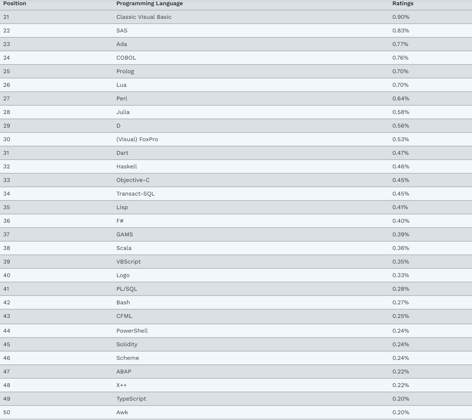
常用编程语言排行与应用场景汇总(2023.10)
文章目录 编程语言排行一、Python二、C三、C四、Java五、C#六、JavaScript七、VB(Visual Basic)八、PHP九、SQL十、ASM(Assembly Language)十一、Go十二、Scratch十三、Delphi/Object Pascal十四、MATLAB十五、Swift十六、Fortran…...
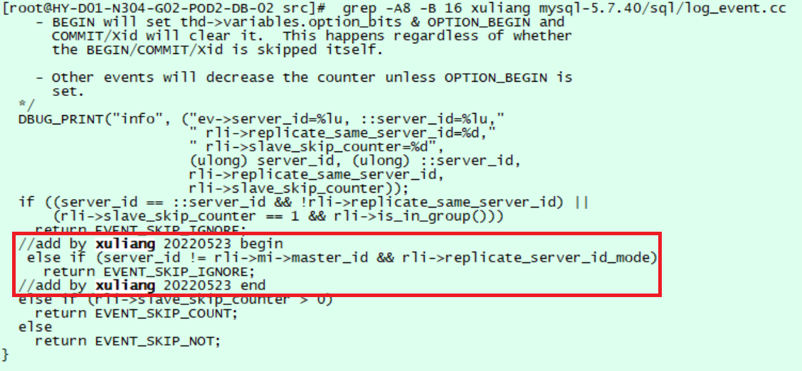
基于 MySQL 多通道主主复制的机房容灾方案
文章中介绍了多种 MySQL 高可用技术,并介绍了根据自身需求选择多通道主主复制技术的过程和注意事项。 作者:徐良,现任中国移动智慧家庭运营中心数据库高级经理,多年数据库运维优化经验,历任华为、一线互联网公司高级 D…...
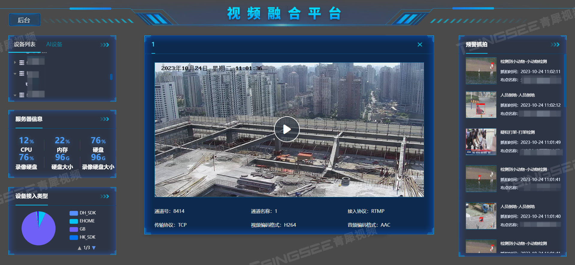
视频汇聚平台EasyCVR分发的流如何进行token鉴权?具体步骤是什么?
视频监控EasyCVR平台能在复杂的网络环境中,将分散的各类视频资源进行统一汇聚、整合、集中管理,在视频监控播放上,TSINGSEE青犀视频安防监控汇聚平台可支持1、4、9、16个画面窗口播放,可同时播放多路视频流,也能支持视…...
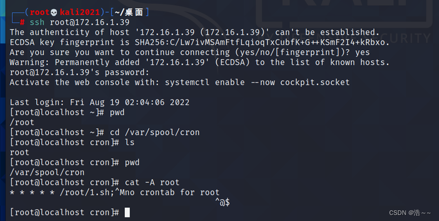
B-5:网络安全事件响应
B-5:网络安全事件响应 任务环境说明: 服务器场景:Server2216(开放链接) 用户名:root密码:123456 1.黑客通过网络攻入本地服务器,通过特殊手段在系统中建立了多个异常进程,找出启动异常进程的脚本,并将其绝对路径作为Flag值提交; 通过nmap扫描我们发现开启了22端口,…...

第17期 | GPTSecurity周报
GPTSecurity是一个涵盖了前沿学术研究和实践经验分享的社区,集成了生成预训练 Transformer(GPT)、人工智能生成内容(AIGC)以及大型语言模型(LLM)等安全领域应用的知识。在这里,您可以…...

透视俄乌网络战之五:俄乌网络战的总结
透视俄乌网络战之一:数据擦除软件 透视俄乌网络战之二:Conti勒索软件集团(上) 透视俄乌网络战之三:Conti勒索软件集团(下) 透视俄乌网络战之四:西方科技巨头的力量 俄乌网络战总结 1…...
深度学习之基于Pytorch卷积神经网络的图像分类系统
欢迎大家点赞、收藏、关注、评论啦 ,由于篇幅有限,只展示了部分核心代码。 文章目录 一项目简介二、功能三、图像分类系统四. 总结 一项目简介 基于PyTorch卷积神经网络的图像分类系统是一种应用深度学习技术来实现图像分类任务的系统。本摘要将对该系统…...

外观专利怎么申请?申请外观专利需要的资料有哪些?
专利分为发明专利、实用新型专利和外观设计专利三类。 我国专利法规定,发明专利的保护期限最长,为自申请日起20年。同时,由于需要进行实质审查,发明专利的审查周期也相对较长,往往需要2年甚至更长时间才能获得授权。 随…...

【Amazon】跨AWS账号资源授权存取访问
文章目录 一、实验框架图二、实验过程说明三、实验演示过程1、在A账号中创建S3存储桶2、在A账号创建S3存储桶访问策略3、在A账号创建信任开发账号的角色4、在B账号为用户添加内联策略5、在B账号中切换角色,以访问A账号中的S3资源 四、实验总结 一、实验框架图 本次…...
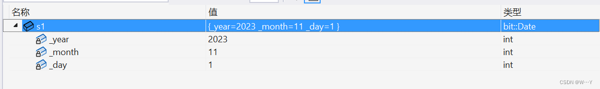
探索C++中的不变之美:const与构造函数的深度剖析
W...Y的主页😊 代码仓库分享💕 🍔前言: 关于C的博客中,我们已经了解了六个默认函数中的四个,分别是构造函数、析构函数、拷贝构造函数以及函数的重载。但是这些函数都是有返回值与参数的。提到参数与返回…...

DDoS类型攻击对企业造成的危害
超级科技实验室的一项研究发现,每十家企业中,有四家(39%)企业没有做好准备应对DDoS攻击,保护自身安全。且不了解应对这类攻击最有效的保护手段是什么。 由于缺乏相关安全知识和保护,使得企业面临巨大的风险。 当黑客发动DDoS攻击…...

深入理解JVM虚拟机第十五篇:虚拟机栈常见异常以及如何设置虚拟机栈的大小
大神链接:作者有幸结识技术大神孙哥为好友,获益匪浅。现在把孙哥视频分享给大家。 孙哥链接:孙哥个人主页 作者简介:一个颜值99分,只比孙哥差一点的程序员 本专栏简介:话不多说,让我们一起干翻JavaScript 本文章简介:话不多说,让我们讲清楚JavaScript里边的Math 文章目…...

Rocketmq5延时消息最大时间
背景 Rocketmq5中支持延时消息的时间,通过Message.setDelayTimeSec可以设置延时消息的精确时间。 问题 当设置时间超过3天时出现异常 org.apache.rocketmq.client.exception.MQBrokerException: CODE: 13 DESC: timer message illegal, the delay time should no…...
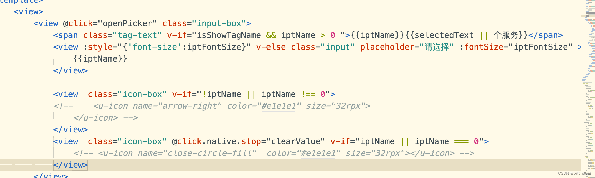
uniapp @click点击事件在新版chrome浏览器点击没反应
问题描述 做项目时,有一个弹出选择的组件,怎么点都不出来,最开始还以为是业务逻辑限制了不能点击。后来才发现别人的电脑可以点出来,老版本的浏览器也可以点出来,最后定位到是新版的chrome就不行了 这是我的浏览器版本…...

beanDefinition读取器
编程式定义 BeanDefinition:自定义一个BeanDefinition, AbstractBeanDefinition beanDefinition BeanDefinitionBuilder.genericBeanDefinition().getBeanDefinition(); 设置beanClass 注册到容器中 B…...

Godot4地图分层绘制实战:从图层混乱到专业场景管理的避坑指南
Godot4地图分层绘制实战:从图层混乱到专业场景管理的避坑指南当你第一次在Godot4中完成一个复杂场景的TileMap绘制时,那种成就感无与伦比。但随着场景复杂度提升,你是否遇到过这些头疼问题:角色明明站在树后却被树叶遮挡ÿ…...

Agent 一接文档批注就开始改错位置:从 Annotation Anchor 到 Suggestion Scope 的工程实战
Agent 对接文档协作平台时,批注是最危险的操作之一。生产环境里,Agent 收到"在第三段加批注"的指令,结果批注挂到第二段末尾,甚至覆盖已有评论。更隐蔽的是,Agent 以作者 A 登录,批注却显示作者 …...

5分钟掌握文件完整性验证:HashCalculator终极免费批量哈希计算工具指南
5分钟掌握文件完整性验证:HashCalculator终极免费批量哈希计算工具指南 【免费下载链接】HashCalculator 哈希值计算工具,批量计算/批量校验/查找重复文件/改变哈希值等,支持集成到系统右键菜单 项目地址: https://gitcode.com/gh_mirrors/…...

Apple Silicon Mac 电池管理的终极解决方案:Battery Toolkit 完整指南
Apple Silicon Mac 电池管理的终极解决方案:Battery Toolkit 完整指南 【免费下载链接】Battery-Toolkit Control the platform power state of your Apple Silicon Mac. 项目地址: https://gitcode.com/gh_mirrors/ba/Battery-Toolkit 在当今移动办公时代&a…...

亿万富翁不再相信比特币
亿万富翁首次公开称不再相信比特币的「数字黄金」叙事。对比特币而言,或许是一个重要转折点。5月22日,亿万富翁投资者马克库班表示, 在对比特币作为抵御法币疲软和地缘政治不稳定对冲工具的作用失去信心后, 他已经卖掉大部分比特币持仓。净资产约为100亿…...

VMware Workstation Pro 17许可证密钥:技术深度解析与最佳实践指南
VMware Workstation Pro 17许可证密钥:技术深度解析与最佳实践指南 【免费下载链接】VMware-Workstation-Pro-17-Licence-Keys Free VMware Workstation Pro 17 full license keys. Weve meticulously organized thousands of keys, catering to all major versions…...

告别窗口遮挡:Topit如何让macOS多任务效率提升3倍
告别窗口遮挡:Topit如何让macOS多任务效率提升3倍 【免费下载链接】Topit Pin any window to the top of your screen / 在Mac上将你的任何窗口强制置顶 项目地址: https://gitcode.com/gh_mirrors/to/Topit 你是否曾经因为窗口重叠而频繁切换应用࿱…...

Redis Bitmap的隐藏用法:从“优惠券防超领”到“大数据去重”的实战避坑指南
Redis Bitmap的隐藏用法:从“优惠券防超领”到“大数据去重”的实战避坑指南 在数据密集型的现代应用中,如何高效处理海量数据的唯一性校验和状态标记,一直是开发者面临的挑战。Redis的Bitmap数据结构以其极低的内存消耗和O(1)时间复杂度的位…...

Hotkey Detective:3步快速定位Windows快捷键冲突的终极指南
Hotkey Detective:3步快速定位Windows快捷键冲突的终极指南 【免费下载链接】hotkey-detective A small program for investigating stolen key combinations under Windows 7 and later. 项目地址: https://gitcode.com/gh_mirrors/ho/hotkey-detective 你是…...

从一次PR被拒说起:我是如何用Git Upstream优雅同步Gitee Fork仓库的
从一次PR被拒说起:我是如何用Git Upstream优雅同步Gitee Fork仓库的 那天下午,当我满怀期待地打开Gitee通知,看到的却是项目维护者冰冷的回复:"PR存在大量冲突,请先同步最新代码"。作为一个刚接触开源贡献的…...