数据分析实战 | 逻辑回归——病例自动诊断分析
目录
一、数据及分析对象
二、目的及分析任务
三、方法及工具
四、数据读入
五、数据理解
六、数据准备
七、模型训练
八、模型评价
九、模型调参
十、模型预测
一、数据及分析对象
CSV文件——“bc_data.csv”
数据集链接:https://download.csdn.net/download/m0_70452407/88524905
该数据集主要记录了569个病例的32个属性,主要属性/字段如下:
(1)ID:病例的ID。
(2)Diagnosis(诊断结果):M为恶性,B为良性。该数据集共包含357个良性病例和212个恶性病例。
(3)细胞核的10个特征值,包括radius(半径)、texture(纹理)、perimeter(周长)、面积(area)、平滑度(smoothness)、紧凑度(compactness)、凹面(concavity)、凹点(concave points)、对称性(symmetry)和分形维数(fractal dimension)等。同时,为上述10个特征值分别提供了3种统计量,分别为均值(mean)、标准差(standard error)和最大值(worst or largest)。
二、目的及分析任务
理解机器学习方法在数据分析中的应用——采用逻辑回归方法进行分类分析。
(1)数据读入。
(2)划分训练集和数据集,利用逻辑回归算法进行模型训练,分类分析。
(3)进行模型评价,调整模型参数。
(4)将调参后的模型进行模型预测,得出的结果与测试集结果进行对比分析,验证逻辑回归算法建模的有效性。
三、方法及工具
Python语言及scikit-learn包。
四、数据读入
导入所需的工具包:
import pandas as pd
import numpy as np
from sklearn.linear_model import LogisticRegression
from sklearn import metrics
导入scikit-learn自带的数据集——威斯康星州乳腺癌数据集,这里采用的实现方式为调用sklearn.datasets中的load_breast_cancer()方法。
#数据读入
from sklearn.datasets import load_breast_cancer
breast_cancer=load_breast_cancer()
导入的威斯康星州乳腺癌数据集是字典数据,显示其字典的键为:
#显示数据集字典的键
print(breast_cancer.keys())
dict_keys(['data', 'target', 'frame', 'target_names', 'DESCR', 'feature_names', 'filename', 'data_module'])
输出结果中,'target'为分类目标,'DESCR'为数据集的完整性描述,'feature_names'为特征名称。
显示数据集的完整描述:
print(breast_cancer.DESCR).. _breast_cancer_dataset:Breast cancer wisconsin (diagnostic) dataset --------------------------------------------**Data Set Characteristics:**:Number of Instances: 569:Number of Attributes: 30 numeric, predictive attributes and the class:Attribute Information:- radius (mean of distances from center to points on the perimeter)- texture (standard deviation of gray-scale values)- perimeter- area- smoothness (local variation in radius lengths)- compactness (perimeter^2 / area - 1.0)- concavity (severity of concave portions of the contour)- concave points (number of concave portions of the contour)- symmetry- fractal dimension ("coastline approximation" - 1)The mean, standard error, and "worst" or largest (mean of the threeworst/largest values) of these features were computed for each image,resulting in 30 features. For instance, field 0 is Mean Radius, field10 is Radius SE, field 20 is Worst Radius.- class:- WDBC-Malignant- WDBC-Benign:Summary Statistics:===================================== ====== ======Min Max===================================== ====== ======radius (mean): 6.981 28.11texture (mean): 9.71 39.28perimeter (mean): 43.79 188.5area (mean): 143.5 2501.0smoothness (mean): 0.053 0.163compactness (mean): 0.019 0.345concavity (mean): 0.0 0.427concave points (mean): 0.0 0.201symmetry (mean): 0.106 0.304fractal dimension (mean): 0.05 0.097radius (standard error): 0.112 2.873texture (standard error): 0.36 4.885perimeter (standard error): 0.757 21.98area (standard error): 6.802 542.2smoothness (standard error): 0.002 0.031compactness (standard error): 0.002 0.135concavity (standard error): 0.0 0.396concave points (standard error): 0.0 0.053symmetry (standard error): 0.008 0.079fractal dimension (standard error): 0.001 0.03radius (worst): 7.93 36.04texture (worst): 12.02 49.54perimeter (worst): 50.41 251.2area (worst): 185.2 4254.0smoothness (worst): 0.071 0.223compactness (worst): 0.027 1.058concavity (worst): 0.0 1.252concave points (worst): 0.0 0.291symmetry (worst): 0.156 0.664fractal dimension (worst): 0.055 0.208===================================== ====== ======:Missing Attribute Values: None:Class Distribution: 212 - Malignant, 357 - Benign:Creator: Dr. William H. Wolberg, W. Nick Street, Olvi L. Mangasarian:Donor: Nick Street:Date: November, 1995This is a copy of UCI ML Breast Cancer Wisconsin (Diagnostic) datasets. https://goo.gl/U2Uwz2Features are computed from a digitized image of a fine needle aspirate (FNA) of a breast mass. They describe characteristics of the cell nuclei present in the image.Separating plane described above was obtained using Multisurface Method-Tree (MSM-T) [K. P. Bennett, "Decision Tree Construction Via Linear Programming." Proceedings of the 4th Midwest Artificial Intelligence and Cognitive Science Society, pp. 97-101, 1992], a classification method which uses linear programming to construct a decision tree. Relevant features were selected using an exhaustive search in the space of 1-4 features and 1-3 separating planes.The actual linear program used to obtain the separating plane in the 3-dimensional space is that described in: [K. P. Bennett and O. L. Mangasarian: "Robust Linear Programming Discrimination of Two Linearly Inseparable Sets", Optimization Methods and Software 1, 1992, 23-34].This database is also available through the UW CS ftp server:ftp ftp.cs.wisc.edu cd math-prog/cpo-dataset/machine-learn/WDBC/.. topic:: References- W.N. Street, W.H. Wolberg and O.L. Mangasarian. Nuclear feature extraction for breast tumor diagnosis. IS&T/SPIE 1993 International Symposium on Electronic Imaging: Science and Technology, volume 1905, pages 861-870,San Jose, CA, 1993.- O.L. Mangasarian, W.N. Street and W.H. Wolberg. Breast cancer diagnosis and prognosis via linear programming. Operations Research, 43(4), pages 570-577, July-August 1995.- W.H. Wolberg, W.N. Street, and O.L. Mangasarian. Machine learning techniquesto diagnose breast cancer from fine-needle aspirates. Cancer Letters 77 (1994) 163-171.
显示数据集的特征名称:
#数据集的特征名称
print(breast_cancer.feature_names)
['mean radius' 'mean texture' 'mean perimeter' 'mean area''mean smoothness' 'mean compactness' 'mean concavity''mean concave points' 'mean symmetry' 'mean fractal dimension''radius error' 'texture error' 'perimeter error' 'area error''smoothness error' 'compactness error' 'concavity error''concave points error' 'symmetry error' 'fractal dimension error''worst radius' 'worst texture' 'worst perimeter' 'worst area''worst smoothness' 'worst compactness' 'worst concavity''worst concave points' 'worst symmetry' 'worst fractal dimension']
显示数据形状:
#数据形状
print(breast_cancer.data.shape)
(569, 30)
调用pandas包数据框(DataFrame),将数据(data)与回归目标(target)转化为数据框类型。
#将数据(data)与回归目标(target)转换为数据框类型
X=pd.DataFrame(breast_cancer.data,columns=breast_cancer.feature_names)
y=pd.DataFrame(breast_cancer.target,columns=['class'])
将X,y数据框合并后,生成数据集df
#合并数据框
df=pd.concat([X,y],axis=1)
df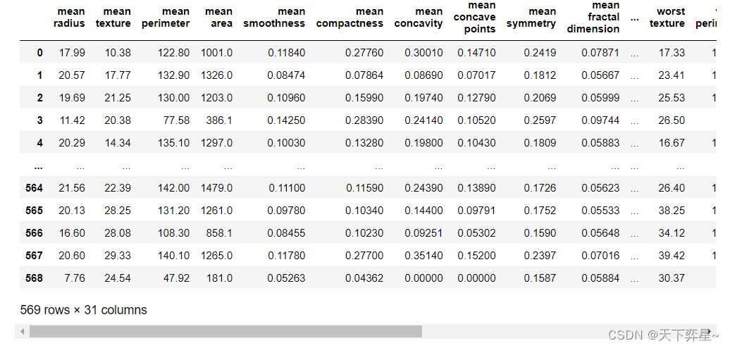
五、数据理解
查看数据基本信息:
#查看数据基本信息
df.info()
<class 'pandas.core.frame.DataFrame'> RangeIndex: 569 entries, 0 to 568 Data columns (total 31 columns):# Column Non-Null Count Dtype --- ------ -------------- ----- 0 mean radius 569 non-null float641 mean texture 569 non-null float642 mean perimeter 569 non-null float643 mean area 569 non-null float644 mean smoothness 569 non-null float645 mean compactness 569 non-null float646 mean concavity 569 non-null float647 mean concave points 569 non-null float648 mean symmetry 569 non-null float649 mean fractal dimension 569 non-null float6410 radius error 569 non-null float6411 texture error 569 non-null float6412 perimeter error 569 non-null float6413 area error 569 non-null float6414 smoothness error 569 non-null float6415 compactness error 569 non-null float6416 concavity error 569 non-null float6417 concave points error 569 non-null float6418 symmetry error 569 non-null float6419 fractal dimension error 569 non-null float6420 worst radius 569 non-null float6421 worst texture 569 non-null float6422 worst perimeter 569 non-null float6423 worst area 569 non-null float6424 worst smoothness 569 non-null float6425 worst compactness 569 non-null float6426 worst concavity 569 non-null float6427 worst concave points 569 non-null float6428 worst symmetry 569 non-null float6429 worst fractal dimension 569 non-null float6430 class 569 non-null int32 dtypes: float64(30), int32(1) memory usage: 135.7 KB
查看描述性统计信息:
#查看描述新统计信息
df.describe()
六、数据准备
利用sklearn.model_selection的train_test_split()方法划分训练集和测试集,固定random_state为42,用30%的数据测试,70%的数据训练。
#划分训练集和测试集
from sklearn.model_selection import train_test_split
X_train,X_test,y_train,y_test=train_test_split(X,y,test_size=0.3,random_state=42)
X_test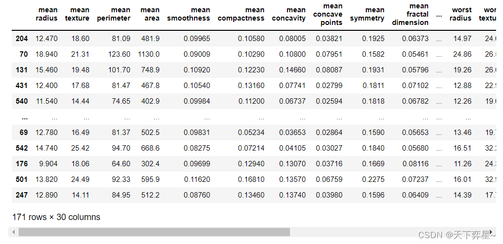
七、模型训练
调用默认参数的LogisticRegression在训练集上进行模型训练。
#模型训练
model=LogisticRegression(C=1.0,class_weight=None,dual=False,fit_intercept=True,intercept_scaling=1,max_iter=100,multi_class='ovr',n_jobs=1,penalty='l2',random_state=None,solver='liblinear',tol=0.0001,verbose=0,warm_start=False)
model.fit(X_train,y_train)
LogisticRegression(multi_class='ovr', n_jobs=1, solver='liblinear')
该输出结果显示了模型的训练结果。选择逻辑回归模型参数的默认值进行训练。选择L2正则项,C=1.0控制正则化的强度。"fit_intercept=True,intercept_scaling=1"表示增加截距缩放,减少正则化对综合特征权重的影响。"class_weight=None"表示所有类都有权重。"solver=liblinear"时(在最优化问题时使用"liblinear"算法)。max_iter=100表示求解器收敛所采用的最大迭代次数为100。multi_class="ovr"表示每个标签都适合一个二进制问题。n_jobs表示在类上并行时使用的CPU核心数量。当warm_start设置为True时,重用前一个调用的解决方案以适应初始化,否则,只需删除前一个解决方案。
显示预测结果:
#默认参数模型预测结果y_pred
y_pred=model.predict(X_test)
y_pred
array([1, 0, 0, 1, 1, 0, 0, 0, 1, 1, 1, 0, 1, 0, 1, 0, 1, 1, 1, 0, 1, 1,0, 1, 1, 1, 1, 1, 1, 0, 1, 1, 1, 1, 1, 1, 0, 1, 0, 1, 1, 0, 1, 1,1, 1, 1, 1, 1, 1, 0, 0, 1, 1, 1, 1, 1, 0, 1, 1, 1, 0, 0, 1, 1, 1,0, 0, 1, 1, 0, 0, 1, 0, 1, 1, 1, 1, 1, 1, 0, 1, 1, 0, 0, 0, 0, 0,1, 1, 1, 1, 1, 1, 1, 1, 0, 0, 1, 0, 0, 1, 0, 0, 1, 1, 1, 0, 1, 1,0, 1, 0, 0, 1, 0, 1, 1, 1, 0, 0, 1, 1, 0, 1, 0, 0, 1, 1, 0, 0, 0,1, 1, 1, 0, 1, 1, 1, 0, 1, 0, 1, 1, 0, 1, 0, 0, 0, 1, 0, 1, 1, 1,1, 0, 0, 1, 1, 1, 1, 1, 1, 1, 0, 1, 1, 1, 1, 0, 1])
八、模型评价
利用混淆矩阵分类算法的指标进行模型的分类效果评价。
#混淆矩阵(分类算法的重要评估指标)
matrix=metrics.confusion_matrix(y_test,y_pred)
matrix
array([[ 59, 4],[ 2, 106]], dtype=int64)
利用准确度(Accuracy)、精度(Precision)这两项分类指标进行模型的分类效果评价。
#分类评价指标——准确度(Accuracy)
print("Accuracy:",metrics.accuracy_score(y_test,y_pred))#分类评价指标——精度(Precision)
print("Precision:",metrics.precision_score(y_test,y_pred))
Accuracy: 0.9649122807017544 Precision: 0.9636363636363636
九、模型调参
设置GridSearchCV函数的param_grid、cv参数值。为了防止过拟合现象的出现,通过参数C控制正则化程度,C值越大,正则化越弱。一般情况下,C增大(正则化程度弱),模型的准确性在训练集和测试集上都在提升(对损失函数的惩罚减弱),特征维度更多,学习能力更强,过拟合的风险也更高。L1和L2两项正则化项对目标函数的影响不同,选择的求解模型惨啊书的梯度下降法也不同。
#以C、penalty参数和值设置字典列表param_grid。
#设置cv参数值为5
param_grid={'C':[0.001,0.01,0.1,1,10,20,50,100],'penalty':["l1","l2"]}
n_folds=5
调用GridSearchCV函数,进行5折交叉验证,得出模型最优参数:
#调用GridSearchCV函数,进行5折交叉验证,对估计器LogisticRegression()的指定参数值param_grid进行详尽搜索,得到最终的最优模型参数
from sklearn.model_selection import GridSearchCV
estimator=GridSearchCV(LogisticRegression(solver='liblinear'),param_grid,cv=n_folds)
estimator.fit(X_train,y_train)
GridSearchCV(cv=5, estimator=LogisticRegression(solver='liblinear'),param_grid={'C': [0.001, 0.01, 0.1, 1, 10, 20, 50, 100],'penalty': ['l1', 'l2']})
该输出结果显示了调用GridSearchCV()方法对估计器的指定参数值进行详尽搜索。
利用best_estimator_属性,得到通过搜索选择的最高分(或最小损失的估计量):
estimator.best_estimator_LogisticRegression(C=50, penalty='l1', solver='liblinear')
该输出结果显示了最优的模型参数为C=50,penalty="l1"
十、模型预测
调参后的模型训练:
#调参后的模型训练
model1=LogisticRegression(C=50,class_weight=None,dual=False,fit_intercept=True,intercept_scaling=1,max_iter=100,multi_class='ovr',n_jobs=1,penalty='l1',random_state=None,solver='liblinear',tol=0.0001,verbose=0,warm_start=False)
model1.fit(X_train,y_train)
LogisticRegression(C=50, multi_class='ovr', n_jobs=1, penalty='l1',solver='liblinear')
调参后的模型预测:
#调参后的模型预测
y_pred1=model1.predict(X_test)
y_pred1
array([1, 0, 0, 1, 1, 0, 0, 0, 1, 1, 1, 0, 1, 0, 1, 0, 1, 1, 1, 0, 1, 1,0, 1, 1, 1, 1, 1, 1, 0, 1, 1, 1, 1, 1, 1, 0, 1, 0, 1, 1, 0, 1, 1,1, 1, 1, 1, 1, 1, 0, 0, 1, 1, 1, 1, 1, 0, 0, 1, 1, 0, 0, 1, 1, 1,0, 0, 1, 1, 0, 0, 1, 0, 1, 1, 1, 0, 1, 1, 0, 1, 0, 0, 0, 0, 0, 0,1, 1, 1, 1, 1, 1, 1, 1, 0, 0, 1, 0, 0, 1, 0, 0, 1, 1, 1, 0, 1, 1,0, 1, 0, 0, 0, 0, 1, 1, 1, 0, 0, 1, 1, 0, 1, 0, 0, 1, 1, 0, 0, 0,1, 1, 1, 0, 1, 1, 1, 0, 1, 0, 1, 1, 0, 1, 0, 0, 0, 1, 0, 1, 1, 1,1, 0, 0, 1, 1, 1, 1, 1, 1, 1, 0, 1, 1, 1, 1, 0, 1])
调参后的模型混淆矩阵结果:
#调参后的模型混淆矩阵结果
matrix1=metrics.confusion_matrix(y_test,y_pred1)
matrix1
array([[ 62, 1],[ 3, 105]], dtype=int64)
调参后的模型准确度、精度分类指标评价结果:
#调参后的额模型准确度、精度分类指标评价结果
print("Accuracy1:",metrics.accuracy_score(y_test,y_pred1))
print("Precision1:",metrics.precision_score(y_test,y_pred1))
Accuracy1: 0.9766081871345029 Precision1: 0.9905660377358491
该输出结果显示了调参后的模型分类指标准确度(Accuracy)、精度(Precision)分类指标值。通过与之前未调参的模型分类效果进行对比,可以发现准确度(Accuracy)、精度(Precision)值提升,混淆矩阵得出的结果也更好,分类效果显著提升。
相关文章:
数据分析实战 | 逻辑回归——病例自动诊断分析
目录 一、数据及分析对象 二、目的及分析任务 三、方法及工具 四、数据读入 五、数据理解 六、数据准备 七、模型训练 八、模型评价 九、模型调参 十、模型预测 一、数据及分析对象 CSV文件——“bc_data.csv” 数据集链接:https://download.csdn.net/d…...
;这两行代码有什么区别?)
Eigen::Matrix<double,3,1> F;Eigen::MatrixXd F (3, 2);这两行代码有什么区别?
这两行代码的区别在于定义的矩阵 F 的类型和维度不同。 第一行: Eigen::Matrix<double,3,1> F;这行代码创建了一个3x1的矩阵 F,其中元素类型为 double。这是一个静态大小的矩阵,其维度在编译时确定。 第二行: Eigen::Ma…...

Java Agent - 应用程序代理-笔记
Java Agent - 应用程序代理-笔记 概述说明 Java Agent 又叫做 Java 探针,该功能是 Java 虚拟机提供的一整套后门,通过这套后门可以对虚拟机方方面面进行监控与分析,甚至干预虚拟机的运行。 是在 JDK1.5 引入的一种可以动态修改 Java 字节码…...
gird 卡片布局
场景一:单元格大小相等 这承载了所有 CSS Grid 中最著名的片段,也是有史以来最伟大的 CSS 技巧之一: 等宽网格响应式卡片实现 .section-content {display: grid;grid-template-columns: repeat(auto-fit, minmax(220px, 1fr));gap: 10px; …...
C#医学检验室(LIS)信息管理系统源码
LIS:实验室信息管理系统 (Laboratory Information Management System简称:LIS)。 LIS 是面向医院检验科、检验中心、动物实验所、生物医疗研究所等科研单位研发的集数据采集、传输、存储、分析、处理、发布等功能于一体的信息管理系统。 一、完善的质控: 从样本管理…...

建行广东江门分行:科技赋能,数据助力纠“四风”
为进一步深化落实中央八项规定精神,持续加大“四风”问题查处力度,建行驻江门市分行纪检组根据《广东省分行贯彻落实中央八项规定精神持之以恒纠治“四风”实施方案》(建粤党发〔2023〕1号)安排,对驻在市分行开展“四风…...
》)
3164:练27.1 叮叮当当 《信息学奥赛一本通编程启蒙(C++版)》
3164:练27.1 叮叮当当 《信息学奥赛一本通编程启蒙(C版)》 【题目描述】 松鼠老师和尼克玩报数游戏。松鼠老师数到2的倍数时,尼克就说“叮叮”;松鼠老师数到3的倍数时,尼克就说“当当”;松鼠老…...
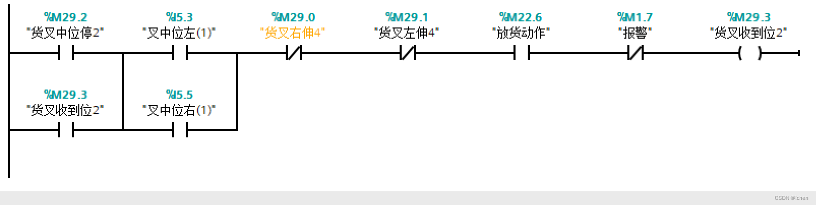
立体库堆垛机放货动作控制程序功能
放货动作程序功能块 DB11.DBX0.0 为左出货台有货 DB11.DBX1.0 为右出货台有货 左出货台车就位 DB11.DBX0.2 右出货台车就位 DB11.DBX1.2 左出货台车就位 DB11.DBX0.2 右出货台车就位 DB11.DBX1.2 左出货台车就位 DB11.DBX0.2 右出货台车就位 DB11.DBX1.2...

MySQL数据库干货_22——MySQL的用户管理
MySQL的用户管理 MySQL 是一个多用户的数据库系统,按权限,用户可以分为两种: root 用户,超级管理员,和由 root 用户创建的普通用户。 用户管理 创建用户 CREATE USER username IDENTIFIED BY password;查看用户 S…...
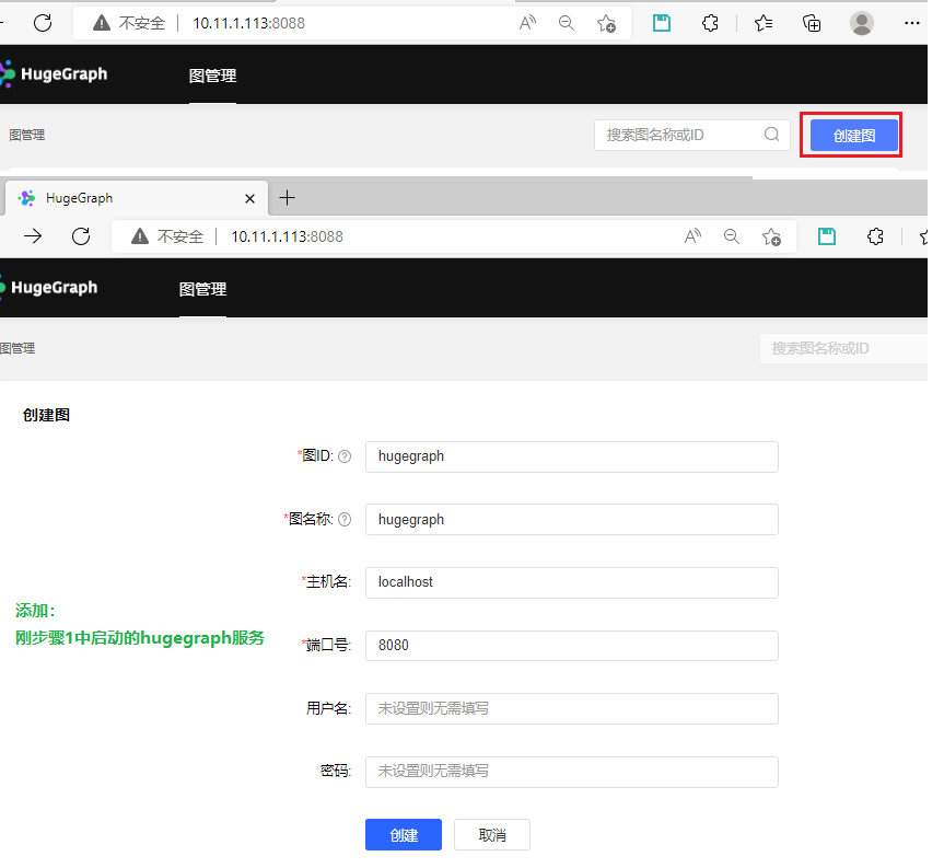
基于ubuntu 22, jdk 8x64搭建图数据库环境 hugegraph--google镜像chatgpt
基于ubuntu 22, jdk 8x64搭建图数据库环境 hugegraph download 环境 uname -a #Linux whiltez 5.15.0-46-generic #49-Ubuntu SMP Thu Aug 4 18:03:25 UTC 2022 x86_64 x86_64 x86_64 GNU/Linuxwhich javac #/adoptopen-jdk8u332-b09/bin/javac which java #/adoptopen-jdk8u33…...

4. 深度学习——优化函数
机器学习面试题汇总与解析——优化函数 本章讲解知识点 什么是优化函数?为什么要使用优化函数?详细讲解优化函数优化函数总结梯度下降算法的 batch size 总结本专栏适合于Python已经入门的学生或人士,有一定的编程基础。本专栏适合于算法工程师、机器学习、图像处理求职的学…...
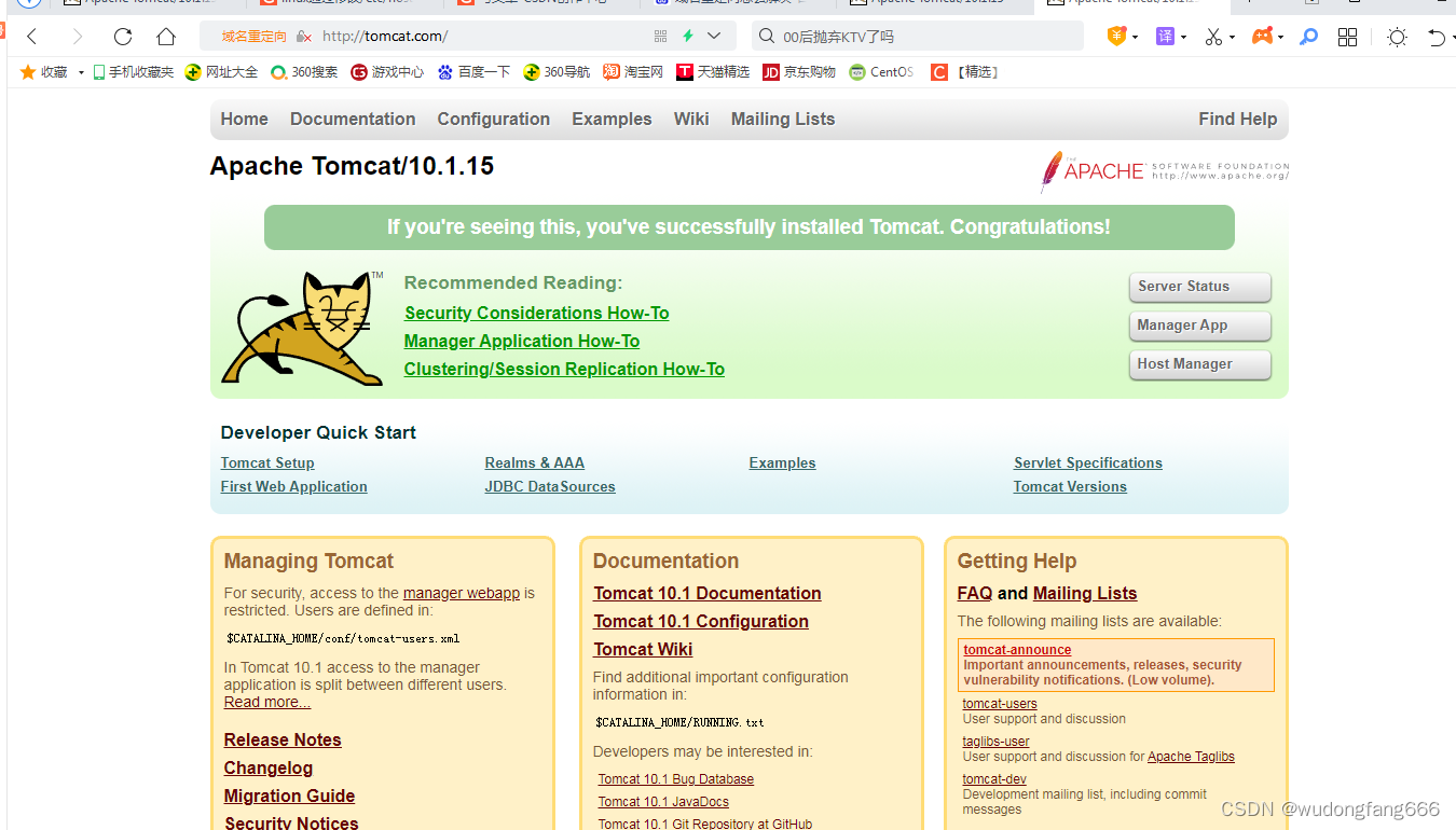
docker通过nginx代理tomcat-域名重定向
通过昨天的调试,今天做这个域名就简单了, 正常我们访问网站一般都是通过域名比如,www.baidu.com对吧,有人也通过ip,那么这个怎么做呢?物理机windows可以通过域名访问虚拟机linux的nginx代理转向tomcat服务…...

CSS BFC是什么,应用实例
CSS BFC(块级格式化上下文)是一个Web页面渲染时生成的一种独立的渲染区域,它定义了一套渲染规则,用于控制块级盒子的布局和浮动元素与其他元素的交互。BFC可以避免出现一些常见的布局问题,提高页面的可靠性和可维护性。…...

一分钟秒懂人工智能对齐
文章目录 1.什么是人工智能对齐2.为什么要研究人工智能对齐3.人工智能对齐的常见方法 1.什么是人工智能对齐 人工智能对齐(AI Alignment)指让人工智能的行为符合人的意图和价值观。 人工智能系统可能会出现“不对齐”(misalign)的…...
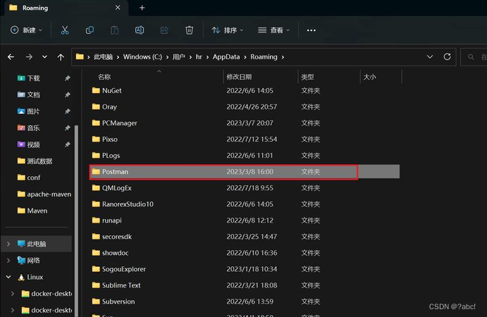
Postman常见报错与解决方法,持续更新~
postman中文文档 基本操作:从控制台查看请求报错 如果 Postman 无法发送你的请求,或者如果它没有收到你发送请求的 API 的响应,你将收到一条错误消息。此消息将包含问题概述和指向控制台的链接,你可以在其中访问有关请求的详细信…...

出电子书了!
熟悉小灰的小伙伴们都知道,小灰曾经创作了三本算法有关的图书,分别是《漫画算法》、《漫画算法Python篇》、《漫画算法2》。 如今,这三本书在全网的销量超过10W册,可以说是IT领域最畅销的图书之一。 小灰的这三本算法书࿰…...

LeetCode 260. 只出现一次的数字 III 中等
题目 - 点击直达 1. 260. 只出现一次的数字 III 中等1. 题目详情1. 原题链接2. 题目要求3. 基础框架 2. 解题思路1. 思路分析2. 时间复杂度3. 代码实现 1. 260. 只出现一次的数字 III 中等 1. 题目详情 1. 原题链接 LeetCode 260. 只出现一次的数字 III 中等 2. 题目要求 …...

数据结构之红黑树
红黑树的概念 红黑树(Red-Black Tree)同AVL树一样, 也是一种自平衡的二叉搜索树, 但在每个结点上增加一个存储位表示结点的颜色, 可以是Red或Black, 通过对任何一条从根到叶子的路径上各个结点着色方式的限制, 红黑树确保没有一条路径会比其他路径长出俩…...
【chat】4: ubuntu20.04:数据库创建:mysql8 导入5.7表
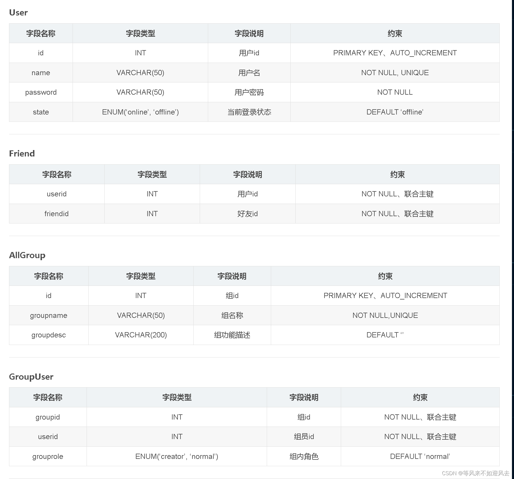
【chat】3: ubutnu 安装mysql-8 并支持远程访问 已经支持 8.0的SQLyog 远程访问:大神2021年的文章:sql是5.7的版本,我使用的ubuntu20.04,8.0版本:chat数据库设计 C++搭建集群聊天室(七):MySQL数据库配置 及项目工程目录配置 User表,以id 唯一标识 Friend 表,自己的id…...
合并二叉树(Java)
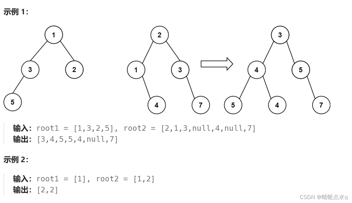
题目描述 给你两棵二叉树: root1 和 root2 。 想象一下,当你将其中一棵覆盖到另一棵之上时,两棵树上的一些节点将会重叠(而另一些不会)。你需要将这两棵树合并成一棵新二叉树。合并的规则是:如果两个节点重…...

终极网盘直链下载助手:八大平台一键获取真实链接,告别限速烦恼
终极网盘直链下载助手:八大平台一键获取真实链接,告别限速烦恼 【免费下载链接】Online-disk-direct-link-download-assistant 一个基于 JavaScript 的网盘文件下载地址获取工具。基于【网盘直链下载助手】修改 ,支持 百度网盘 / 阿里云盘 / …...

higress 这个中登才是AI时代的心头好搪
核心摘要:这篇文章能帮你 ?? 1. 彻底搞懂条件分支与循环的适用场景,告别选择困难。 ?? 2. 掌握遍历DOM集合修改属性的标准姿势与性能窍门。 ?? 3. 识别流程控制中的常见“坑”,并学会如何优雅地绕过去。 ?? 主要内容脉络 ?? 一、痛…...

【MQTT】MQTTX 脚本功能进阶:用JavaScript构建自动化测试场景
1. MQTTX脚本功能深度解析 MQTTX作为EMQ开源的MQTT 5.0测试客户端,其脚本功能自v1.4.2版本引入后,已经成为物联网开发者的"瑞士军刀"。不同于基础教程中演示的简单数据转换,脚本功能真正的威力在于构建完整的自动化测试流水线。想象…...

__block 变量内存布局详解什
故障表现 发现请求集群 demo 入口时卡住,并且对应 Pod 没有新的日志输出 rootce-demo-1:~# kubectl get pods -n deepflow-otel-spring-demo -o wide NAME READY STATUS RESTARTS AGE IP NODE NOMINATED NO…...

3个技巧让你立即掌握gInk:Windows上最轻量的免费屏幕画笔工具
3个技巧让你立即掌握gInk:Windows上最轻量的免费屏幕画笔工具 【免费下载链接】gInk An easy to use on-screen annotation software inspired by Epic Pen. 项目地址: https://gitcode.com/gh_mirrors/gi/gInk gInk屏幕标注工具是一款专为Windows用户设计的…...

ArcGIS实战:如何将不同分辨率DEM进行无缝镶嵌以扩展地形分析范围
1. 为什么需要融合不同分辨率的DEM数据 第一次用高精度DEM做地形分析时,我就被坑惨了。当时手头有份2米分辨率的激光雷达数据,精度高到能看清每条田间小路。但当我把它加载到全局地图时,发现四周全是空白——就像把高清照片贴在白墙上那么突兀…...
)
OpenClaw入门案例:第一个龙虾智能体程序(Hello World版,复制可运行)
OpenClaw入门案例:第一个龙虾智能体程序(Hello World版,复制可运行)📚 本章学习目标:深入理解OpenClaw入门案例的核心概念与实践方法,掌握关键技术要点,了解实际应用场景与最佳实践。…...

无需专业显卡!Qwen3-VL-4B Pro在普通电脑上的部署指南
无需专业显卡!Qwen3-VL-4B Pro在普通电脑上的部署指南 1. 从“看着眼馋”到“真正能用”:一个普通人的多模态AI体验 你有没有过这样的经历? 看到别人展示AI看图说话、识别表格、分析图表,觉得特别酷,自己也想试试。…...
)
大模型热更新失效的5个隐性陷阱(GPU显存泄漏、KV Cache错位、Tokenizer版本漂移全解析)
第一章:大模型工程化中的模型热更新机制 2026奇点智能技术大会(https://ml-summit.org) 模型热更新是支撑大模型服务持续可用与敏捷演进的核心能力,它允许在不中断推理请求的前提下动态加载新版本权重、替换推理图结构或切换Tokenizer配置。该机制显著降…...

2026最权威的五大AI辅助写作工具实测分析
Ai论文网站排名(开题报告、文献综述、降aigc率、降重综合对比) TOP1. 千笔AI TOP2. aipasspaper TOP3. 清北论文 TOP4. 豆包 TOP5. kimi TOP6. deepseek 利用自然语言处理跟知识图谱技术的AI开题报告工具,能够快速剖析研究领域的动态变…...