原始GAN-pytorch-生成MNIST数据集（代码）

原始GAN生成MNIST数据集

原理很简单，可以参考原理部分原始GAN-pytorch-生成MNIST数据集（原理）

import os
import time
import torch
from tqdm import tqdm
from torch import nn, optim
from torch.utils.data import DataLoader
from torchvision import datasets
from torchvision import transforms
from torchvision.utils import save_image
import sys 
from pathlib import Path
import matplotlib.pyplot as plt
import numpy as np
from PIL import Image

1. Data loading and preparing

测试使用loadlocal_mnist加载数据

from mlxtend.data import loadlocal_mnist
train_data_path = "../data/MNIST/train-images.idx3-ubyte"
train_label_path = "../data/MNIST/train-labels.idx1-ubyte"
test_data_path = "../data/MNIST/t10k-images.idx3-ubyte"
test_label_path = "../data/MNIST/t10k-labels.idx1-ubyte"train_data,train_label = loadlocal_mnist(images_path = train_data_path,labels_path = train_label_path
)
train_data.shape,train_label.shape

((60000, 784), (60000,))

import matplotlib.pyplot as pltimg,ax = plt.subplots(3,3,figsize=(9,9))
plt.subplots_adjust(hspace=0.4,wspace=0.4)
for i in range(3):for j in range(3):num = np.random.randint(0,train_label.shape[0])ax[i][j].imshow(train_data[num].reshape((28,28)),cmap="gray")ax[i][j].set_title(train_label[num],fontdict={"fontsize":20})
plt.show()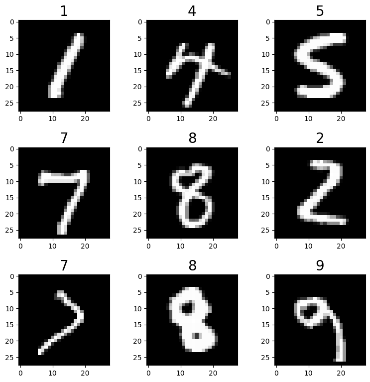

2. Dataset and Model parameter

构造pytorch数据集datasets和数据加载器dataloader

input_size = [1, 28, 28]
batch_size = 128
Epoch = 1000
GenEpoch = 1
in_channel = 64

from torch.utils.data import Dataset,DataLoader
import numpy as np 
from mlxtend.data import loadlocal_mnist
import torchvision.transforms as transformsclass MNIST_Dataset(Dataset):def __init__(self,train_data_path,train_label_path,transform=None):train_data,train_label = loadlocal_mnist(images_path = train_data_path,labels_path = train_label_path)self.train_data = train_dataself.train_label = train_label.reshape(-1)self.transform=transformdef __len__(self):return self.train_label.shape[0] def __getitem__(self,index):if torch.is_tensor(index):index = index.tolist()images = self.train_data[index,:].reshape((28,28))labels = self.train_label[index]if self.transform:images = self.transform(images)return images,labelstransform_dataset =transforms.Compose([transforms.ToTensor()]
)
MNIST_dataset = MNIST_Dataset(train_data_path=train_data_path,train_label_path=train_label_path,transform=transform_dataset)  
MNIST_dataloader = DataLoader(dataset=MNIST_dataset,batch_size=batch_size,shuffle=True,drop_last=False)

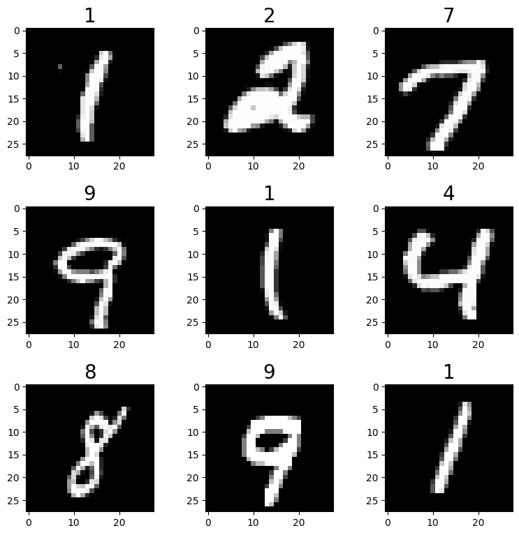
img,ax = plt.subplots(3,3,figsize=(9,9))
plt.subplots_adjust(hspace=0.4,wspace=0.4)
for i in range(3):for j in range(3):num = np.random.randint(0,train_label.shape[0])ax[i][j].imshow(MNIST_dataset[num][0].reshape((28,28)),cmap="gray")ax[i][j].set_title(MNIST_dataset[num][1],fontdict={"fontsize":20})
plt.show()

3. Result save path

time_now = time.strftime('%Y-%m-%d-%H_%M_%S', time.localtime(time.time()))
log_path = f'./log/{time_now}'
os.makedirs(log_path)
os.makedirs(f'{log_path}/image')
os.makedirs(f'{log_path}/image/image_all')

device = 'cuda' if torch.cuda.is_available() else 'cpu'
print(f'using device: {device}')

using device: cuda

4. Model define

import torch
from torch import nn class Discriminator(nn.Module):def __init__(self,input_size,inplace=True):super(Discriminator,self).__init__()c,h,w = input_sizeself.dis = nn.Sequential(nn.Linear(c*h*w,512),  # 输入特征数为784，输出为512nn.BatchNorm1d(512),nn.LeakyReLU(0.2),  # 进行非线性映射nn.Linear(512, 256),  # 进行一个线性映射nn.BatchNorm1d(256),nn.LeakyReLU(0.2),nn.Linear(256, 1),nn.Sigmoid()  # 也是一个激活函数，二分类问题中，# sigmoid可以班实数映射到【0,1】，作为概率值，# 多分类用softmax函数)def forward(self,x):b,c,h,w = x.size()x = x.view(b,-1)x = self.dis(x)x = x.view(-1)return x class Generator(nn.Module):def __init__(self,in_channel):super(Generator,self).__init__() # 调用父类的构造方法self.gen = nn.Sequential(nn.Linear(in_channel, 128),nn.LeakyReLU(0.2),nn.Linear(128, 256),nn.BatchNorm1d(256),nn.LeakyReLU(0.2),nn.Linear(256, 512),nn.BatchNorm1d(512),nn.LeakyReLU(0.2),nn.Linear(512, 1024),nn.BatchNorm1d(1024),nn.LeakyReLU(0.2),nn.Linear(1024, 784),nn.Tanh())def forward(self,x):res = self.gen(x)return res.view(x.size()[0],1,28,28)D = Discriminator(input_size=input_size)
G = Generator(in_channel=in_channel)
D.to(device)
G.to(device)
D,G

(Discriminator((dis): Sequential((0): Linear(in_features=784, out_features=512, bias=True)(1): BatchNorm1d(512, eps=1e-05, momentum=0.1, affine=True, track_running_stats=True)(2): LeakyReLU(negative_slope=0.2)(3): Linear(in_features=512, out_features=256, bias=True)(4): BatchNorm1d(256, eps=1e-05, momentum=0.1, affine=True, track_running_stats=True)(5): LeakyReLU(negative_slope=0.2)(6): Linear(in_features=256, out_features=1, bias=True)(7): Sigmoid())),Generator((gen): Sequential((0): Linear(in_features=64, out_features=128, bias=True)(1): LeakyReLU(negative_slope=0.2)(2): Linear(in_features=128, out_features=256, bias=True)(3): BatchNorm1d(256, eps=1e-05, momentum=0.1, affine=True, track_running_stats=True)(4): LeakyReLU(negative_slope=0.2)(5): Linear(in_features=256, out_features=512, bias=True)(6): BatchNorm1d(512, eps=1e-05, momentum=0.1, affine=True, track_running_stats=True)(7): LeakyReLU(negative_slope=0.2)(8): Linear(in_features=512, out_features=1024, bias=True)(9): BatchNorm1d(1024, eps=1e-05, momentum=0.1, affine=True, track_running_stats=True)(10): LeakyReLU(negative_slope=0.2)(11): Linear(in_features=1024, out_features=784, bias=True)(12): Tanh())))

6. Training

criterion = nn.BCELoss()
D_optimizer = torch.optim.Adam(D.parameters(),lr=0.0003)
G_optimizer = torch.optim.Adam(G.parameters(),lr=0.0003)
D.train()
G.train()
gen_loss_list = []
dis_loss_list = []for epoch in range(Epoch):with tqdm(total=MNIST_dataloader.__len__(),desc=f'Epoch {epoch+1}/{Epoch}')as pbar:gen_loss_avg = []dis_loss_avg = []index = 0for batch_idx,(img,_) in enumerate(MNIST_dataloader):img = img.to(device)# the output labelvalid = torch.ones(img.size()[0]).to(device)fake = torch.zeros(img.size()[0]).to(device)# Generator inputG_img = torch.randn([img.size()[0],in_channel],requires_grad=True).to(device)# ------------------Update Discriminator------------------# forwardG_pred_gen = G(G_img)G_pred_dis = D(G_pred_gen.detach())R_pred_dis = D(img)# the misfitG_loss = criterion(G_pred_dis,fake)R_loss = criterion(R_pred_dis,valid)dis_loss = (G_loss+R_loss)/2dis_loss_avg.append(dis_loss.item())# backwardD_optimizer.zero_grad()dis_loss.backward()D_optimizer.step()# ------------------Update Optimizer------------------# forwardG_pred_gen = G(G_img)G_pred_dis = D(G_pred_gen)# the misfitgen_loss = criterion(G_pred_dis,valid)gen_loss_avg.append(gen_loss.item())# backwardG_optimizer.zero_grad()gen_loss.backward()G_optimizer.step()# save figureif index % 200 == 0 or index + 1 == MNIST_dataset.__len__():save_image(G_pred_gen, f'{log_path}/image/image_all/epoch-{epoch}-index-{index}.png')index += 1# ------------------进度条更新------------------pbar.set_postfix(**{'gen-loss': sum(gen_loss_avg) / len(gen_loss_avg),'dis-loss': sum(dis_loss_avg) / len(dis_loss_avg)})pbar.update(1)save_image(G_pred_gen, f'{log_path}/image/epoch-{epoch}.png')filename = 'epoch%d-genLoss%.2f-disLoss%.2f' % (epoch, sum(gen_loss_avg) / len(gen_loss_avg), sum(dis_loss_avg) / len(dis_loss_avg))torch.save(G.state_dict(), f'{log_path}/{filename}-gen.pth')torch.save(D.state_dict(), f'{log_path}/{filename}-dis.pth')# 记录损失gen_loss_list.append(sum(gen_loss_avg) / len(gen_loss_avg))dis_loss_list.append(sum(dis_loss_avg) / len(dis_loss_avg))# 绘制损失图像并保存plt.figure(0)plt.plot(range(epoch + 1), gen_loss_list, 'r--', label='gen loss')plt.plot(range(epoch + 1), dis_loss_list, 'r--', label='dis loss')plt.legend()plt.xlabel('epoch')plt.ylabel('loss')plt.savefig(f'{log_path}/loss.png', dpi=300)plt.close(0)

Epoch 1/1000: 100%|██████████| 469/469 [00:11<00:00, 41.56it/s, dis-loss=0.456, gen-loss=1.17] 
Epoch 2/1000: 100%|██████████| 469/469 [00:11<00:00, 42.34it/s, dis-loss=0.17, gen-loss=2.29] 
Epoch 3/1000: 100%|██████████| 469/469 [00:10<00:00, 43.29it/s, dis-loss=0.0804, gen-loss=3.11]
Epoch 4/1000: 100%|██████████| 469/469 [00:11<00:00, 40.74it/s, dis-loss=0.0751, gen-loss=3.55]
Epoch 5/1000: 100%|██████████| 469/469 [00:12<00:00, 39.01it/s, dis-loss=0.105, gen-loss=3.4]  
Epoch 6/1000: 100%|██████████| 469/469 [00:11<00:00, 39.95it/s, dis-loss=0.112, gen-loss=3.38]
Epoch 7/1000: 100%|██████████| 469/469 [00:11<00:00, 40.16it/s, dis-loss=0.116, gen-loss=3.42]
Epoch 8/1000: 100%|██████████| 469/469 [00:11<00:00, 42.51it/s, dis-loss=0.124, gen-loss=3.41]
Epoch 9/1000: 100%|██████████| 469/469 [00:11<00:00, 40.95it/s, dis-loss=0.136, gen-loss=3.41]
Epoch 10/1000: 100%|██████████| 469/469 [00:11<00:00, 39.59it/s, dis-loss=0.165, gen-loss=3.13]
Epoch 11/1000: 100%|██████████| 469/469 [00:11<00:00, 40.28it/s, dis-loss=0.176, gen-loss=3.01]
Epoch 12/1000: 100%|██████████| 469/469 [00:12<00:00, 37.60it/s, dis-loss=0.19, gen-loss=2.94] 
Epoch 13/1000: 100%|██████████| 469/469 [00:11<00:00, 39.17it/s, dis-loss=0.183, gen-loss=2.95]
Epoch 14/1000: 100%|██████████| 469/469 [00:12<00:00, 38.51it/s, dis-loss=0.182, gen-loss=3.01]
Epoch 15/1000: 100%|██████████| 469/469 [00:10<00:00, 44.58it/s, dis-loss=0.186, gen-loss=2.95]
Epoch 16/1000: 100%|██████████| 469/469 [00:10<00:00, 44.08it/s, dis-loss=0.198, gen-loss=2.89]
Epoch 17/1000: 100%|██████████| 469/469 [00:10<00:00, 45.11it/s, dis-loss=0.187, gen-loss=2.99]
Epoch 18/1000: 100%|██████████| 469/469 [00:10<00:00, 44.98it/s, dis-loss=0.183, gen-loss=3.03]
Epoch 19/1000: 100%|██████████| 469/469 [00:10<00:00, 46.68it/s, dis-loss=0.187, gen-loss=2.98]
Epoch 20/1000: 100%|██████████| 469/469 [00:10<00:00, 46.12it/s, dis-loss=0.192, gen-loss=3]   
Epoch 21/1000: 100%|██████████| 469/469 [00:10<00:00, 46.80it/s, dis-loss=0.193, gen-loss=3.01]
Epoch 22/1000: 100%|██████████| 469/469 [00:10<00:00, 45.86it/s, dis-loss=0.186, gen-loss=3.04]
Epoch 23/1000: 100%|██████████| 469/469 [00:10<00:00, 46.00it/s, dis-loss=0.17, gen-loss=3.2]  
Epoch 24/1000: 100%|██████████| 469/469 [00:10<00:00, 46.41it/s, dis-loss=0.173, gen-loss=3.19]
Epoch 25/1000: 100%|██████████| 469/469 [00:10<00:00, 45.15it/s, dis-loss=0.19, gen-loss=3.1]  
Epoch 26/1000: 100%|██████████| 469/469 [00:10<00:00, 44.26it/s, dis-loss=0.178, gen-loss=3.16]
Epoch 27/1000: 100%|██████████| 469/469 [00:10<00:00, 45.14it/s, dis-loss=0.187, gen-loss=3.17]
Epoch 28/1000:   1%|▏         | 6/469 [00:00<00:12, 38.20it/s, dis-loss=0.184, gen-loss=3.04]---------------------------------------------------------------------------

7. predict

input_size = [3, 32, 32]
in_channel = 64
gen_para_path = './log/2023-02-11-17_52_12/epoch999-genLoss1.21-disLoss0.40-gen.pth'
dis_para_path = './log/2023-02-11-17_52_12/epoch999-genLoss1.21-disLoss0.40-dis.pth'
device = 'cuda' if torch.cuda.is_available() else 'cpu'
gen = Generator_Transpose(in_channel=in_channel).to(device)
dis = DiscriminatorLinear(input_size=input_size).to(device)
gen.load_state_dict(torch.load(gen_para_path, map_location=device))
gen.eval()
# 随机生成一组数据
G_img = torch.randn([1, in_channel, 1, 1], requires_grad=False).to(device)
# 放入网路
G_pred = gen(G_img)
G_dis = dis(G_pred)
print('generator-dis:', G_dis)
# 图像显示
G_pred = G_pred[0, ...]
G_pred = G_pred.detach().cpu().numpy()
G_pred = np.array(G_pred * 255)
G_pred = np.transpose(G_pred, [1, 2, 0])
G_pred = Image.fromarray(np.uint8(G_pred))
G_pred.show()