【PyTorch】教程:对抗学习实例生成
ADVERSARIAL EXAMPLE GENERATION
研究推动 ML 模型变得更快、更准、更高效。设计和模型的安全性和鲁棒性经常被忽视,尤其是面对那些想愚弄模型故意对抗时。
本教程将提供您对 ML 模型的安全漏洞的认识,并将深入了解对抗性机器学习这一热门话题。在图像中添加难以察觉的扰动会导致模型性能的显著不同,鉴于这是一个教程,我们将通过图像分类器的示例来探讨这个主题。具体来说,我们将使用第一种也是最流行的攻击方法之一,快速梯度符号攻击( FGSM )来欺骗 MNIST 分类器。
Threat Model (攻击模型)
在论文中,有许多类型的对抗攻击,每种攻击都有不同的目标和攻击者的知识假设。然而,总的来说,首要目标是向输入数据添加最小数量的扰动,以导致期望的错误分类。攻击者的知识有几种假设,其中两种是: white-box (白盒)和 black-box (黑盒);白盒攻击假定攻击者具有对模型的完整知识和访问权限,包括体系结构、输入、输出和权重。黑盒攻击假设攻击者只能访问模型的输入和输出,并且对底层架构或权重一无所知。还有几种类型的目标,包括 misclassification (错误分类)和 source/target misclassification 源/目标错误分类。错误分类的目标意味着对手只希望输出分类错误,而不在乎新的分类是什么。源/目标错误分类意味着对手希望更改最初属于特定源类别的图像,从而将其分类为特定目标类别。
Fast Gradient Sign Attack
FGSM 攻击是白盒攻击,目标是错误分类。
迄今为止最早也是最流行的的对抗攻击是 Fast Gradient Sign Attack, FGSM (Explaining and Harnessing Adversarial Examples),这种攻击非常强大, 也很直观。它旨在利用神经网络的学习方式,即梯度来攻击神经网络。这个想法很简单,而不是通过基于反向传播梯度调整权重来最小化损失,而是基于相同的反向传播梯度来调整输入数据以最大化损失。换句话说,攻击使用输入数据的损失梯度,然后调整输入数据以最大化损失。
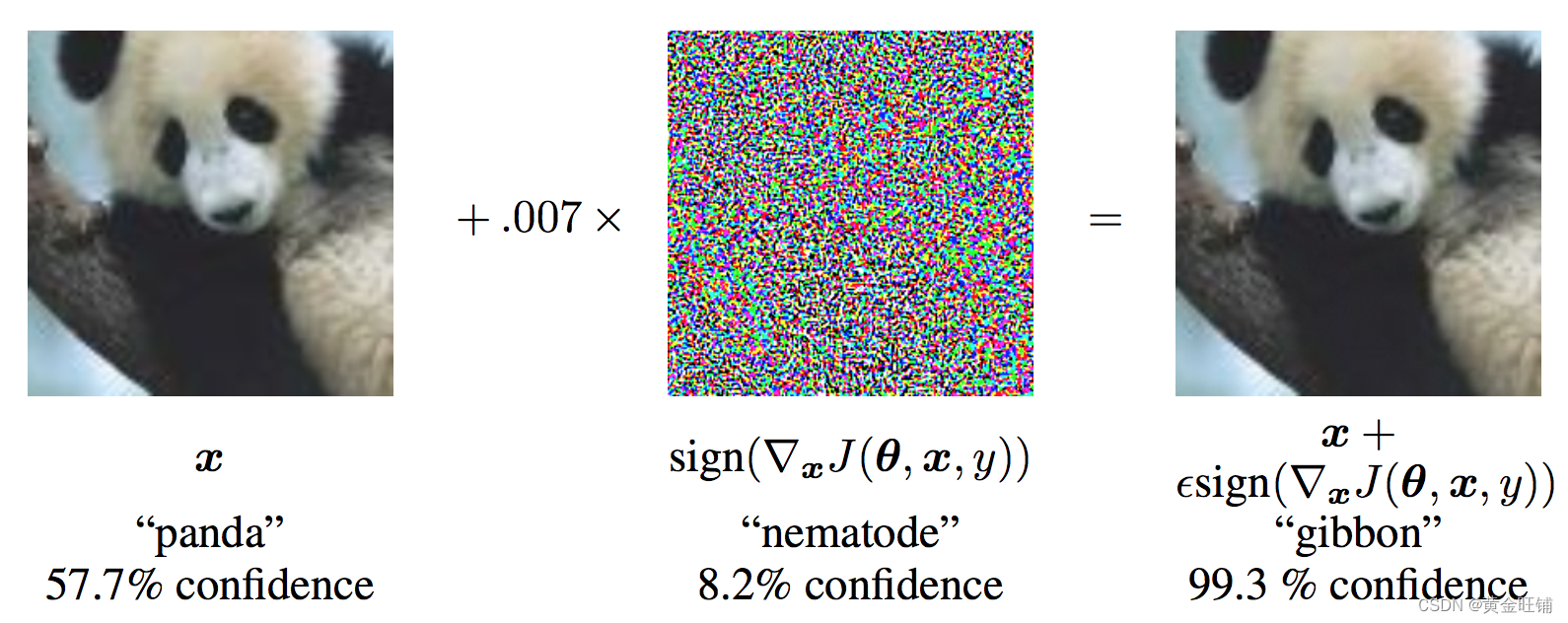
从图中可以看出, xxx 是被正确分类为 panda 的原始图像,yyy 是 xxx 的正确标签,θ\thetaθ 代表的是模型参数,$ J(\theta, x, y)$ 是训练网络的 loss 。攻击反向传播梯度到输入数据计算 ∇xJ(θ,x,y)\nabla_x J(\theta, x, y)∇xJ(θ,x,y) , 然后利用很小的步长 ( ϵ\epsilonϵ 或 0.007 ) 在某个方向上最大化损失(例如: sign(∇xJ(θ,x,y))sign(\nabla_x J(\theta, x, y))sign(∇xJ(θ,x,y)) ),最后的扰动图像 x′x'x′ 最后被错误分类为 gibbon, 实际上图像还是 panda 。
import torch
import torch.nn as nn
import torch.nn.functional as F
import torch.optim as optim
from torchvision import datasets, transforms
import numpy as np
import matplotlib.pyplot as plt from six.moves import urllib
opener = urllib.request.build_opener()
opener.addheaders = [('User-agent', 'Mozilla/5.0')]
urllib.request.install_opener(opener)
Implementation
本节中,我们将讨论教程的输入参数,定义攻击下的模型,以及相关的测试
Inputs
三个输入:
- epsilons: epsilon 列表值,保持 0 在列表中非常重要,代表着原始模型的性能。 epsilon 越大代表着攻击越大。
- pretrained_model: 预训练模型,训练模型的代码在 这里. 也可以直接下载 预训练模型. 因为 google drive 无法下载,所以还可以在 CSDN资源 下载
- use_cuda: 使用 GPU;
Model Under Attack
定义了模型和 DataLoader,初始化模型和加载权重。
class Net(nn.Module):def __init__(self):super(Net, self).__init__()self.conv1 = nn.Conv2d(1, 32, 3, 1)self.conv2 = nn.Conv2d(32, 64, 3, 1)self.dropout1 = nn.Dropout(0.25)self.dropout2 = nn.Dropout(0.5)self.fc1 = nn.Linear(9216, 128)self.fc2 = nn.Linear(128, 10)def forward(self, x):x = self.conv1(x)x = F.relu(x)x = self.conv2(x)x = F.relu(x)x = F.max_pool2d(x, 2)x = self.dropout1(x)x = torch.flatten(x, 1)x = self.fc1(x)x = F.relu(x)x = self.dropout2(x)x = self.fc2(x)output = F.log_softmax(x, dim=1)return outputepsilons = [0, .05, .1, .15, .2, .25, .3]
pretrained_model = "lenet_mnist_model.pt"
use_cuda = True# MNIST Test dataset and dataloader declaration
test_loader = torch.utils.data.DataLoader(datasets.MNIST('../../../datasets', train=False, download=True, transform=transforms.Compose([transforms.ToTensor(),])),batch_size=1, shuffle=True)print("CUDA Available: ", torch.cuda.is_available())
device = torch.device('cuda' if (use_cuda and torch.cuda.is_available()) else 'cpu')# init network
model = Net().to(device)# load the pretrained model
model.load_state_dict(torch.load(pretrained_model, map_location='cpu'))# set the model in evaluation mode. In this case this is for the Dropout layers
model.eval()
CUDA Available:  True
Net((conv1): Conv2d(1, 32, kernel_size=(3, 3), stride=(1, 1))(conv2): Conv2d(32, 64, kernel_size=(3, 3), stride=(1, 1))(dropout1): Dropout(p=0.25, inplace=False)(dropout2): Dropout(p=0.5, inplace=False)(fc1): Linear(in_features=9216, out_features=128, bias=True)(fc2): Linear(in_features=128, out_features=10, bias=True)
)
FGSM Attack (FGSM 攻击)
我们现在定义一个函数创建一个对抗实例,通过对原始输入进行干扰。 fgsm_attack 函数有3个输入,原始输入图像 xxx,像素方向扰动量 ϵ\epsilonϵ ,梯度损失,(例如 ∇xJ(θ,x,y)\nabla_x J(\mathbf{\theta}, \mathbf{x}, y)∇xJ(θ,x,y))
创建干扰图像
perturbedimage=image+epsilon∗sign(datagrad)=x+ϵ∗sign(∇xJ(θ,x,y))perturbed_image=image+epsilon∗sign(data_grad)=x+ϵ∗sign(∇x J(θ,x,y)) perturbedimage=image+epsilon∗sign(datagrad)=x+ϵ∗sign(∇xJ(θ,x,y))
最后,为了保持原始图像的数据范围,干扰图像被缩放到 [0, 1]
# FGSM attack code
def fgsm_attack(image, epsilon, data_grad):# collect the element-wise sign of the data gradientsign_data_grad = data_grad.sign()# create the perturbed image by adjusting each pixel of the input image perturbed_image = image + epsilon * sign_data_grad # adding clipping to maintain [0, 1] range perturbed_image = torch.clamp(perturbed_image, 0, 1)# return the perturbed image return perturbed_image
Testing Function (测试函数)
def test(model, device, test_loader, epsilon):# accuracy countercorrect = 0adv_examples = []# loop over all examples in test set for data, target in test_loader:data, target = data.to(device), target.to(device)# Set requires_grad attribute of tensor. Important for Attackdata.requires_grad = True# output = model(data)init_pred = output.max(1, keepdim=True)[1]# if the initial prediction is wrong, don't botter attacking, just move onif init_pred.item() != target.item():continue # calculate the lossloss = F.nll_loss(output, target)# zero all existing gradmodel.zero_grad()# calculate gradients of model in backward loss loss.backward()# collect datagraddata_grad = data.grad.data # call FGSM attackperturbed_data = fgsm_attack(data, epsilon, data_grad)# reclassify the perturbed image output = model(perturbed_data)# check for success final_pred = output.max(1, keepdim=True)[1]# if final_pred.item() == target.item():correct += 1# special case for saving 0 epsilon examplesif (epsilon == 0) and (len(adv_examples) < 5):adv_ex = perturbed_data.squeeze().detach().cpu().numpy()adv_examples.append((init_pred.item(), final_pred.item(), adv_ex))else:# Save some adv examples for visualization laterif len(adv_examples) < 5:adv_ex = perturbed_data.squeeze().detach().cpu().numpy()adv_examples.append( (init_pred.item(), final_pred.item(), adv_ex) )# Calculate final accuracy for this epsilonfinal_acc = correct/float(len(test_loader))print("Epsilon: {}\tTest Accuracy = {} / {} = {}".format(epsilon, correct, len(test_loader), final_acc))# Return the accuracy and an adversarial examplereturn final_acc, adv_examples
Run Attack (执行攻击)
实现的最后一步是执行攻击,我们针对每个 epsilon 执行全部的 test step,并且保存最终的准确率和一些成功的对抗实例。 ϵ=0\epsilon=0ϵ=0 不执行攻击
accuracies = []
examples = []# Run test for each epsilon
for eps in epsilons:acc, ex = test(model, device, test_loader, eps)accuracies.append(acc)examples.append(ex)
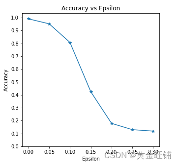
Epsilon: 0	Test Accuracy = 9906 / 10000 = 0.9906
Epsilon: 0.05	Test Accuracy = 9517 / 10000 = 0.9517
Epsilon: 0.1	Test Accuracy = 8070 / 10000 = 0.807
Epsilon: 0.15	Test Accuracy = 4242 / 10000 = 0.4242
Epsilon: 0.2	Test Accuracy = 1780 / 10000 = 0.178
Epsilon: 0.25	Test Accuracy = 1292 / 10000 = 0.1292
Epsilon: 0.3	Test Accuracy = 1180 / 10000 = 0.118
Accuracy vs Epsilon (正确率 VS epsilon)
ϵ\epsilonϵ 增大时,我们期望正确率下降,因为大的 ϵ\epsilonϵ 我们在方向上有大的变换可以最大化 loss. 他们的变换不是线性的,一开始下降的慢,中间下降的快,最后下降的慢。
plt.figure(figsize=(5, 5))
plt.plot(epsilons, accuracies, "*-")
plt.yticks(np.arange(0, 1.1, step=0.1))
plt.xticks(np.arange(0, .35, step=0.05))
plt.title("Accuracy vs Epsilon")
plt.xlabel("Epsilon")
plt.ylabel("Accuracy")
plt.show()
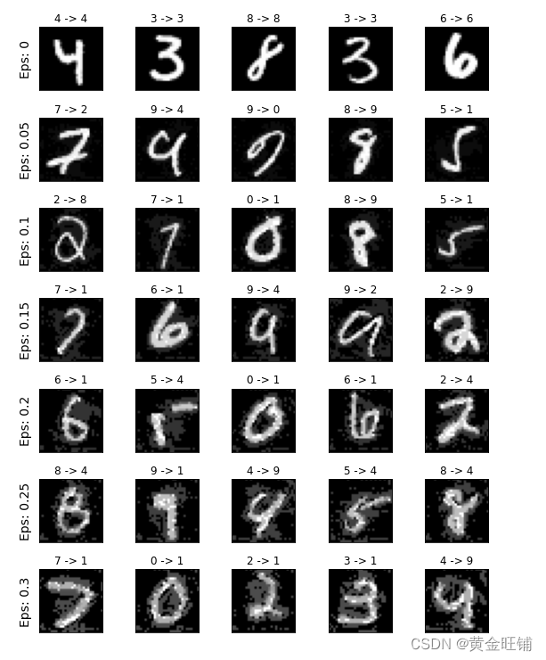
Sample Adversarial Examples (对抗实例)
# Plot several examples of adversarial samples at each epsilon
cnt = 0
plt.figure(figsize=(8,10))
for i in range(len(epsilons)):for j in range(len(examples[i])):cnt += 1plt.subplot(len(epsilons),len(examples[0]),cnt)plt.xticks([], [])plt.yticks([], [])if j == 0:plt.ylabel("Eps: {}".format(epsilons[i]), fontsize=14)orig,adv,ex = examples[i][j]plt.title("{} -> {}".format(orig, adv))plt.imshow(ex, cmap="gray")
plt.tight_layout()
plt.show()
完整代码
import torch
import torch.nn as nn
import torch.nn.functional as F
import torch.optim as optim
from torchvision import datasets, transforms
import numpy as np
import matplotlib.pyplot as plt from six.moves import urllib
opener = urllib.request.build_opener()
opener.addheaders = [('User-agent', 'Mozilla/5.0')]
urllib.request.install_opener(opener) class Net(nn.Module):def __init__(self):super(Net, self).__init__()self.conv1 = nn.Conv2d(1, 32, 3, 1)self.conv2 = nn.Conv2d(32, 64, 3, 1)self.dropout1 = nn.Dropout(0.25)self.dropout2 = nn.Dropout(0.5)self.fc1 = nn.Linear(9216, 128)self.fc2 = nn.Linear(128, 10)def forward(self, x):x = self.conv1(x)x = F.relu(x)x = self.conv2(x)x = F.relu(x)x = F.max_pool2d(x, 2)x = self.dropout1(x)x = torch.flatten(x, 1)x = self.fc1(x)x = F.relu(x)x = self.dropout2(x)x = self.fc2(x)output = F.log_softmax(x, dim=1)return outputepsilons = [0, .05, .1, .15, .2, .25, .3]
pretrained_model = "lenet_mnist_model.pt"
use_cuda = True# MNIST Test dataset and dataloader declaration
test_loader = torch.utils.data.DataLoader(datasets.MNIST('../../../datasets', train=False, download=True, transform=transforms.Compose([transforms.ToTensor(),])),batch_size=1, shuffle=True)print("CUDA Available: ", torch.cuda.is_available())
device = torch.device('cuda' if (use_cuda and torch.cuda.is_available()) else 'cpu')# init network
model = Net().to(device)# load the pretrained model
model.load_state_dict(torch.load(pretrained_model, map_location='cpu'))# set the model in evaluation mode. In this case this is for the Dropout layers
model.eval()# FGSM attack code
def fgsm_attack(image, epsilon, data_grad):# collect the element-wise sign of the data gradientsign_data_grad = data_grad.sign()# create the perturbed image by adjusting each pixel of the input image perturbed_image = image + epsilon * sign_data_grad # adding clipping to maintain [0, 1] range perturbed_image = torch.clamp(perturbed_image, 0, 1)# return the perturbed image return perturbed_imagedef test(model, device, test_loader, epsilon):# accuracy countercorrect = 0adv_examples = []# loop over all examples in test setfor data, target in test_loader:data, target = data.to(device), target.to(device)# Set requires_grad attribute of tensor. Important for Attackdata.requires_grad = True#output = model(data)init_pred = output.max(1, keepdim=True)[1]# if the initial prediction is wrong, don't botter attacking, just move onif init_pred.item() != target.item():continue# calculate the lossloss = F.nll_loss(output, target)# zero all existing gradmodel.zero_grad()# calculate gradients of model in backward lossloss.backward()# collect datagraddata_grad = data.grad.data# call FGSM attackperturbed_data = fgsm_attack(data, epsilon, data_grad)# reclassify the perturbed imageoutput = model(perturbed_data)# check for successfinal_pred = output.max(1, keepdim=True)[1]#if final_pred.item() == target.item():correct += 1# special case for saving 0 epsilon examplesif (epsilon == 0) and (len(adv_examples) < 5):adv_ex = perturbed_data.squeeze().detach().cpu().numpy()adv_examples.append((init_pred.item(), final_pred.item(), adv_ex))else:# Save some adv examples for visualization laterif len(adv_examples) < 5:adv_ex = perturbed_data.squeeze().detach().cpu().numpy()adv_examples.append((init_pred.item(), final_pred.item(), adv_ex))# Calculate final accuracy for this epsilonfinal_acc = correct/float(len(test_loader))print("Epsilon: {}\tTest Accuracy = {} / {} = {}".format(epsilon, correct,len(test_loader), final_acc))# Return the accuracy and an adversarial examplereturn final_acc, adv_examplesaccuracies = []
examples = []# Run test for each epsilon
for eps in epsilons:acc, ex = test(model, device, test_loader, eps)accuracies.append(acc)examples.append(ex)plt.figure(figsize=(5, 5))
plt.plot(epsilons, accuracies, "*-")
plt.yticks(np.arange(0, 1.1, step=0.1))
plt.xticks(np.arange(0, .35, step=0.05))
plt.title("Accuracy vs Epsilon")
plt.xlabel("Epsilon")
plt.ylabel("Accuracy")
plt.show()# Plot several examples of adversarial samples at each epsilon
cnt = 0
plt.figure(figsize=(8, 10))
for i in range(len(epsilons)):for j in range(len(examples[i])):cnt += 1plt.subplot(len(epsilons), len(examples[0]), cnt)plt.xticks([], [])plt.yticks([], [])if j == 0:plt.ylabel("Eps: {}".format(epsilons[i]), fontsize=14)orig, adv, ex = examples[i][j]plt.title("{} -> {}".format(orig, adv))plt.imshow(ex, cmap="gray")
plt.tight_layout()
plt.show()
【参考】
ADVERSARIAL EXAMPLE GENERATION
相关文章:
【PyTorch】教程:对抗学习实例生成
ADVERSARIAL EXAMPLE GENERATION 研究推动 ML 模型变得更快、更准、更高效。设计和模型的安全性和鲁棒性经常被忽视,尤其是面对那些想愚弄模型故意对抗时。 本教程将提供您对 ML 模型的安全漏洞的认识,并将深入了解对抗性机器学习这一热门话题。在图像…...

中国区使用Open AI账号试用Chat GPT指南
最近推出强大的ChatGPT功能,各大程序员使用后发出感叹:程序员要失业了 不过在国内并不支持OpenAI账号注册,多数会提示: OpenAI’s services are not available in your country. 经过一番搜索后,发现如下方案可以完…...
STM32开发(9)----CubeMX配置外部中断
CubeMX配置外部中断前言一、什么是中断1.STM32中断架构体系2.外部中断/事件控制器(EXTI)3.嵌套向量中断控制器(NIVC)二、实验过程1.CubeMX配置2.代码实现3.硬件连接4.实验结果总结前言 本章介绍使用STM32CubeMX对引脚的外部中断进…...
Nextjs了解内容
目录Next.jsnext.js的实现1,nextjs初始化2, 项目结构3, 数据注入getInitialPropsgetServerSidePropsgetStaticProps客户端注入3,CSS Modules4,layout组件5,文件式路由6,BFF层的文件式路由7&…...

从事功能测试1年,裸辞1个月,找不到工作的“我”怎么办?
做功能测试一年多了裸辞职一个月了,大部分公司都要求有自动化测试经验,可是哪来的自动化测试呢? 我要是简历上写了吧又有欺诈性,不写他们给的招聘又要自动化优先,将项目带向自动化不是一个容易的事情,很多…...

机器学习基本原理总结
本文大部分内容参考《深度学习》书籍,从中抽取重要的知识点,并对部分概念和原理加以自己的总结,适合当作原书的补充资料阅读,也可当作快速阅览机器学习原理基础知识的参考资料。 前言 深度学习是机器学习的一个特定分支。我们要想…...
JVET-AC0315:用于色度帧内预测的跨分量Merge模式
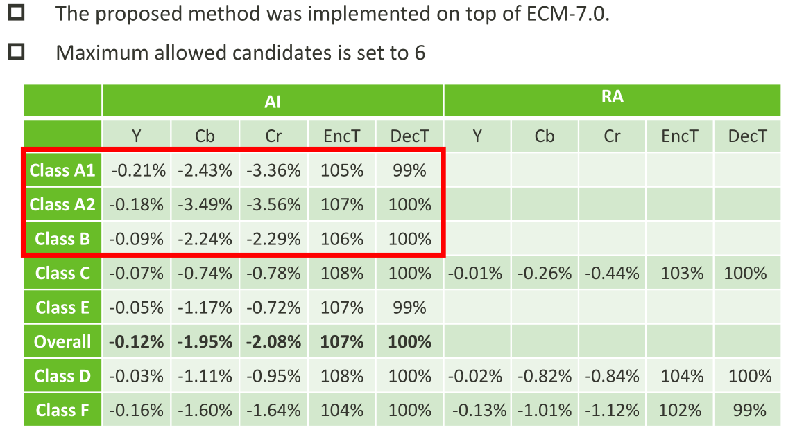
ECM采用了许多跨分量的预测(Cross-componentprediction,CCP)模式,包括跨分量包括跨分量线性模型(CCLM)、卷积跨分量模型(CCCM)和梯度线性模型(GLM)࿰…...
)
Session与Cookie的区别(二)
脸盲症的困扰 小明身为杂货店的店长兼唯一的店员,所有大小事都是他一个人在处理。传统杂货店跟便利商店最大的差别在哪里?在于人情味。 就像是你去菜市场买菜的时候会被说帅哥或美女,或者是去买早餐的时候老板会问你:「一样&#…...

疫情开发,软件测试行情趋势是怎么样的?
如果说,2022年对于全世界来说,都是一场极大的挑战的话;那么,2023年绝对是机遇多多的一年。众所周知,随着疫情在全球范围内逐步得到控制,无论是国际还是国内的环境,都会呈现逐步回升的趋势&#…...

Java中间件描述与使用,面试可以用
myCat 用于切分mysql数据库(为什么要切分:当数据量过大时,mysql查询效率变低) ActiveMQ 订阅,消息推送 swagger 前后端分离,后台接口调式 dubbo 阿里的面向服务RPC框架,为什么要面向服务&#x…...

[OpenMMLab]AI实战营第七节课
语义分割代码实战教学 HRNet 高分辨率神经网络 安装配置 # 选择分支 git branch -a git switch 3.x # 配置环境 conda create -n mmsegmentation python3.8 conda activate mmsegmentation pip install torch1.11.0cu113 torchvision0.12.0cu113 torchaudio0.11.0 --extra-i…...
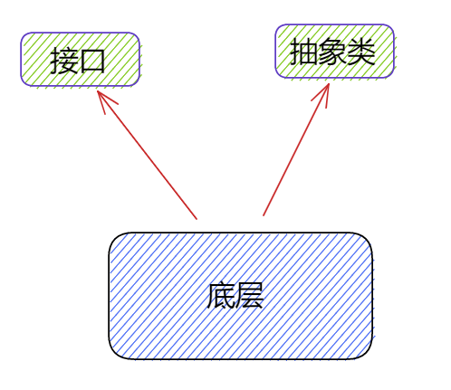
面向对象的设计模式
"万丈高楼平地起,7种模式打地基",模式是一种规范,我们应该站在巨人的肩膀上越看越远,接下来,让我们去仔细了解了解面向对象的7种设计模式7种设计模式设计原则的核心思想:找出应用中可能需要变化之…...

里氏替换原则|SOLID as a rock
文章目录 意图动机:违反里氏替换原则解决方案:C++中里氏替换原则的例子里氏替换原则的优点1、可兼容性2、类型安全3、可维护性在C++中用好LSP的标准费几句话本文是关于 SOLID as Rock 设计原则系列的五部分中的第三部分。 SOLID 设计原则侧重于开发 易于维护、可重用和可扩展…...

【C++】右左法则,指针、函数与数组
右左法则——判断复杂的声明对于一个复杂的声明,可以用右左法则判断它是个什么东西:1.先找到变量名称2.从变量名往右看一个部分,再看变量名左边的一个部分3.有小括号先看小括号里面的,一层一层往外看4.先看到的东西优先级大&#…...

打通数据价值链,百分点数据科学基础平台实现数据到决策的价值转换 | 爱分析调研
随着企业数据规模的大幅增长,如何利用数据、充分挖掘数据价值,服务于企业经营管理成为当下企业数字化转型的关键。 如何挖掘数据价值?企业需要一步步完成数据价值链条的多个环节,如数据集成、数据治理、数据建模、数据分析、数据…...

C++之多态【详细总结】
前言 想必大家都知道面向对象的三大特征:封装,继承,多态。封装的本质是:对外暴露必要的接口,但内部的具体实现细节和部分的核心接口对外是不可见的,仅对外开放必要功能性接口。继承的本质是为了复用&#x…...

ThingsBoard-RPC
1、使用 RPC 功能 ThingsBoard 允许您将远程过程调用 (RPC) 从服务器端应用程序发送到设备,反之亦然。基本上,此功能允许您向/从设备发送命令并接收命令执行的结果。本指南涵盖 ThingsBoard RPC 功能。阅读本指南后,您将熟悉以下主题: RPC 类型;基本 RPC 用例;RPC 客户端…...
java分治算法
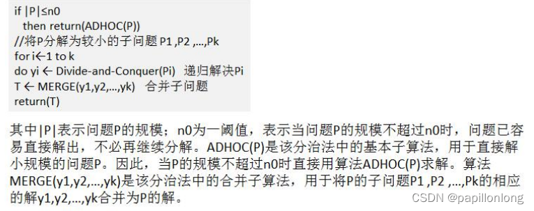
分治算法介绍 分治法是一种很重要的算法。字面上的解释是“分而治之”,就是把一个复杂的问题分成两个或更多的相同或 相似的子问题,再把子问题分成更小的子问题……直到最后子问题可以简单的直接求解,原问题的解即子问题 的解的合并。这个技…...

【Flutter】【Unity】使用 Flutter + Unity 构建(AR 体验工具包)
使用 Flutter Unity 构建(AR 体验工具包)【翻译】 原文:https://medium.com/potato/building-with-flutter-unity-ar-experience-toolkit-6aaf17dbb725 由于屡获殊荣的独立动画工作室 Aardman 与讲故事的风险投资公司 Fictioneers&#x…...
MC0108白给-MC0109新河妇荡杯
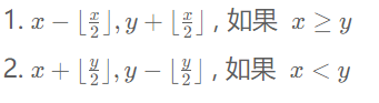
MC0108白给 小码哥和小码妹在玩一个游戏,初始小码哥拥有 x的金钱,小码妹拥有 y的金钱。 虽然他们不在同一个队伍中,但他们仍然可以通过游戏的货币系统进行交易,通过互相帮助以达到共赢的目的。具体来说,在每一回合&a…...
)
第10章 RTOS 感知调试(OpenOCD)
第10章 RTOS 感知调试 导读:在嵌入式开发中,RTOS(实时操作系统)的使用非常普遍。然而当多个线程并发执行时,传统的单线程调试方式无法感知任务切换和线程上下文,给问题定位带来极大困难。OpenOCD 内置了对十余种主流 RTOS 的线程感知调试支持,能够在暂停目标时自动识别所…...

GME-Qwen2-VL-2B实战:手把手教你构建个人多模态知识库
GME-Qwen2-VL-2B实战:手把手教你构建个人多模态知识库 1. 为什么需要多模态知识库? 在日常工作和生活中,我们积累了大量不同类型的数据——文档、图片、截图、笔记等。传统知识管理工具往往只能处理单一类型的数据,要么是纯文本…...

终极指南:如何用org-roam保护敏感笔记的安全与隐私
终极指南:如何用org-roam保护敏感笔记的安全与隐私 【免费下载链接】org-roam Rudimentary Roam replica with Org-mode 项目地址: https://gitcode.com/gh_mirrors/or/org-roam org-roam是一款基于Org-mode的强大知识管理工具,它允许用户创建和管…...

PSIM仿真:基于三相桥式逆变器的下垂控制与LC滤波、SPWM调制
(PSIM)下垂控制-基于三相桥式逆变器的下垂控制,电压电流双闭环,采用LC滤波,SPWM调制方式 1.提供PSIM仿真源文件 2.提供下垂控制原理与下垂系数计算方法 3.中点平衡控制,电压电流双闭环控制 提供参考文献下垂…...

Cursor Pro功能扩展工具:技术原理与开源解决方案
Cursor Pro功能扩展工具:技术原理与开源解决方案 【免费下载链接】cursor-free-vip [Support 0.45](Multi Language 多语言)自动注册 Cursor Ai ,自动重置机器ID , 免费升级使用Pro 功能: Youve reached your trial re…...
)
XZ1851输入电压6-40V 输出电流2.5A 输出电压ADJ(小于39V)
产品概述 XZ1851 是一款内置功率 MOSFET的单片降压型开关模式转换器。 XZ1851在 6-40V 宽输入电源范围内实现2.5 A最大输出电流,并且具有出色的线电压和负载调整率。 XZ1851 采用 PWM 电流模工作模式,环路易于稳定并提供快速的瞬态响应。 XZ1851 外部提供…...

Beyond Compare 5 终极激活指南:本地密钥生成工具完整教程
Beyond Compare 5 终极激活指南:本地密钥生成工具完整教程 【免费下载链接】BCompare_Keygen Keygen for BCompare 5 项目地址: https://gitcode.com/gh_mirrors/bc/BCompare_Keygen Beyond Compare 5 是一款专业的文件对比与合并工具,广泛应用于…...

使用快马平台基于OpenSpec一键生成RESTful API原型,加速后端服务开发
今天想和大家分享一个快速搭建RESTful API原型的经验。最近在开发一个用户管理系统,发现用OpenSpec规范配合InsCode(快马)平台可以省去大量重复工作,特别适合需要快速验证想法的场景。 OpenSpec规范的价值 OpenSpec(也就是OpenAPI规范&#x…...

突破局限:开源微信插件WeChatExtension-ForMac革新体验全解析
突破局限:开源微信插件WeChatExtension-ForMac革新体验全解析 【免费下载链接】WeChatExtension-ForMac Mac微信功能拓展/微信插件/微信小助手(A plugin for Mac WeChat) 项目地址: https://gitcode.com/gh_mirrors/we/WeChatExtension-ForMac 作为Mac用户&a…...
Pixel Fashion Atelier效果实测:在RTX 4090上单图生成耗时稳定在3.2秒内
Pixel Fashion Atelier效果实测:在RTX 4090上单图生成耗时稳定在3.2秒内 1. 测试环境与配置 1.1 硬件配置 本次测试使用的硬件平台为高端游戏工作站: 显卡:NVIDIA RTX 4090 (24GB GDDR6X)处理器:Intel i9-13900K内存ÿ…...