[足式机器人]Part4 南科大高等机器人控制课 Ch09 Dynamics of Open Chains
本文仅供学习使用
本文参考:
B站:CLEAR_LAB
笔者带更新-运动学
课程主讲教师:
Prof. Wei Zhang
南科大高等机器人控制课 Ch09 Dynamics of Open Chains
- 1. Introduction
- 1.1 From Single Rigid Body to Open Chains
- 1.2 Preview of Open-Chain Dynamics
- 1.3 Lagrangian VS. Newton-Euler Methods
- 2. Inverse Dynamics: Recursive Newton-Euler Algorithm(RNEA)
- 2.1 RNEA: Notations
- 2.1.1 RNEA: Velocity and Accel. Propagation(Forward Pass)
- 2.1.2 RNEA: Force Propagation(Backward Pass)
- 2.1.3 Recursive Newton-Euler Algorithm
- 3. Analytical Form of the Dynamics Model
- 3.1 Structures in Dynamic Equation
- 3.2 Properties of Dynamics Model of Multi-Body Systems
- 4. Forward Dynamics Algorithms
- 4.1 Forward Dynamics Problem
- 4.2 Caculations of h and M
- 4.3 Forward Dynamics Algorithms
- 4.4 More Discussions
1. Introduction
1.1 From Single Rigid Body to Open Chains
- Recall Newton-Euler Equation for a single rigid body:
F = d d t H = I A + V ~ ∗ I V \mathcal{F} =\frac{\mathrm{d}}{\mathrm{d}t}\mathcal{H} =\mathcal{I} \mathcal{A} +\tilde{\mathcal{V}}^*\mathcal{I} \mathcal{V} F=dtdH=IA+V~∗IV - Open chains consists of multiple rigid links connected through joints
- Dynamics of adjacent links are coupled
- This lecture: model multi-body dynamics subject to joint constrainsts.
1.2 Preview of Open-Chain Dynamics
-
Equations of Motion are a set of 2nd-order differential equations:
τ = M ( θ ) θ ¨ + c ( θ , θ ˙ ) \tau =M\left( \theta \right) \ddot{\theta}+c\left( \theta ,\dot{\theta} \right) τ=M(θ)θ¨+c(θ,θ˙)
θ ∈ R n \theta \in \mathbb{R} ^n θ∈Rn : vector of joint variables ;
τ ∈ R n \tau \in \mathbb{R} ^n τ∈Rn : vector of joint forces/torques(与之前的符号不一致);
M ( θ ) ∈ R n × n M\left( \theta \right) \in \mathbb{R} ^{n\times n} M(θ)∈Rn×n : mass matrix
c ( θ , θ ˙ ) ∈ R n c\left( \theta ,\dot{\theta} \right) \in \mathbb{R} ^n c(θ,θ˙)∈Rn : forces that lump together centripetal, Coriolis, gravity, friction terms, and torques induced by external forces. These terms depends on θ \theta θ and θ ˙ \dot{\theta} θ˙ -
Forward dynamics : Determine accecleration θ ¨ \ddot{\theta} θ¨ given the state ( θ , θ ˙ ) \left( \theta ,\dot{\theta} \right) (θ,θ˙) and the joint forces/torques
θ ¨ ← F D ( τ , θ , θ ˙ , F e x t ) \ddot{\theta}\gets FD\left( \tau ,\theta ,\dot{\theta},\mathcal{F} _{\mathrm{ext}} \right) θ¨←FD(τ,θ,θ˙,Fext) -
Inverse dynamics : Finding torques/forces given state ( θ , θ ˙ ) \left( \theta ,\dot{\theta} \right) (θ,θ˙) and desired acceleration θ ¨ \ddot{\theta} θ¨ (Given desired motion, find the required torque to generate the desired motion)
τ ← I D ( θ , θ ˙ , θ ¨ , F e x t ) \tau \gets ID\left( \theta ,\dot{\theta},\ddot{\theta},\mathcal{F} _{\mathrm{ext}} \right) τ←ID(θ,θ˙,θ¨,Fext)
1.3 Lagrangian VS. Newton-Euler Methods
- There are typically two ways to derive the equation of motion for an open-chain robot: Lagrangian method and Newton-Euler method
Lagrangian Formulation : Energy-based method ; Dynamic equations in closed form ; Often used for study of dynamic properties and analysis of control methods
Newton-Euler Formulation : Balance of forces/torques ; Dynamic equations in numeric/recuisive form ; Often used for numerical solution of forward/inverse dynamics
We focus on Newton-Euler Formulation
2. Inverse Dynamics: Recursive Newton-Euler Algorithm(RNEA)
2.1 RNEA: Notations

-
Number bodies : 1 to N N N
Parents : p ( i ) : p ( 3 ) = { 2 } , p ( 4 ) = { 2 } p\left( i \right) :p\left( 3 \right) =\left\{ 2 \right\} ,p\left( 4 \right) =\left\{ 2 \right\} p(i):p(3)={2},p(4)={2}
Children : c ( i ) : c ( 2 ) = { 3 , 4 } , c ( 1 ) = { 2 } c\left( i \right) :c\left( 2 \right) =\left\{ 3,4 \right\} ,c\left( 1 \right) =\left\{ 2 \right\} c(i):c(2)={3,4},c(1)={2} -
Joint i i i connects p ( i ) p\left( i \right) p(i) to i i i
-
Frame { i } \left\{ i \right\} {i} attached to body i i i at the joint
-
S i \mathcal{S} _{\mathrm{i}} Si : Spatial velocity (screw axis) of joint i i i
-
V i \mathcal{V} _{\mathrm{i}} Vi and A i \mathcal{A} _{\mathrm{i}} Ai : spatial velocity and acceleration of body i i i
-
F i \mathcal{F} _{\mathrm{i}} Fi : force(wrench) onto body i i i from body p ( i ) p\left( i \right) p(i)
-
Note : By default, all vectors ( S i , V i , F i ) \left( \mathcal{S} _{\mathrm{i}},\mathcal{V} _{\mathrm{i}},\mathcal{F} _{\mathrm{i}} \right) (Si,Vi,Fi) are expressed in local frame { i } \left\{ i \right\} {i}
2.1.1 RNEA: Velocity and Accel. Propagation(Forward Pass)
Goal: Given joint velocity θ ˙ \dot{\theta} θ˙ and acceleration θ ¨ \ddot{\theta} θ¨ , compute the body spatial velocity V i \mathcal{V} _{\mathrm{i}} Vi and spatial acceleration A i \mathcal{A} _{\mathrm{i}} Ai
- Velocity Propagation : V i i = [ X p ( i ) i ] V p ( i ) p ( i ) + S i i θ ˙ i \mathcal{V} _{\mathrm{i}}^{i}=\left[ X_{\mathrm{p}\left( i \right)}^{i} \right] \mathcal{V} _{\mathrm{p}\left( i \right)}^{p\left( i \right)}+\mathcal{S} _{\mathrm{i}}^{i}\dot{\theta}_{\mathrm{i}} Vii=[Xp(i)i]Vp(i)p(i)+Siiθ˙i
- Accel Propagation : A i i = [ X p ( i ) i ] A p ( i ) p ( i ) + V ~ i i S i i θ ˙ i + S i i θ ¨ i \mathcal{A} _{\mathrm{i}}^{i}=\left[ X_{\mathrm{p}\left( i \right)}^{i} \right] \mathcal{A} _{\mathrm{p}\left( i \right)}^{p\left( i \right)}+\tilde{\mathcal{V}}_{\mathrm{i}}^{i}\mathcal{S} _{\mathrm{i}}^{i}\dot{\theta}_{\mathrm{i}}+\mathcal{S} _{\mathrm{i}}^{i}\ddot{\theta}_{\mathrm{i}} Aii=[Xp(i)i]Ap(i)p(i)+V~iiSiiθ˙i+Siiθ¨i
从机架侧开始计算
2.1.2 RNEA: Force Propagation(Backward Pass)
Goal : Given body spatial velocity V i \mathcal{V} _{\mathrm{i}} Vi amd spatial acceleration A i \mathcal{A} _{\mathrm{i}} Ai, compute the joint wrench F i \mathcal{F} _{\mathrm{i}} Fi and the corresponding torque τ i = S i T F i \tau _{\mathrm{i}}={\mathcal{S} _{\mathrm{i}}}^{\mathrm{T}}\mathcal{F} _{\mathrm{i}} τi=SiTFi
{ F i = I i A i + V ~ i ∗ I i V i + ∑ j ∈ c ( i ) F j τ i = S i T F i \begin{cases} \mathcal{F} _{\mathrm{i}}=\mathcal{I} _{\mathrm{i}}\mathcal{A} _{\mathrm{i}}+{\tilde{\mathcal{V}}_{\mathrm{i}}}^*\mathcal{I} _{\mathrm{i}}\mathcal{V} _{\mathrm{i}}+\sum\nolimits_{j\in c\left( i \right)}^{}{\mathcal{F} _{\mathrm{j}}}\\ \tau _{\mathrm{i}}={\mathcal{S} _{\mathrm{i}}}^{\mathrm{T}}\mathcal{F} _{\mathrm{i}}\\ \end{cases} {Fi=IiAi+V~i∗IiVi+∑j∈c(i)Fjτi=SiTFi
从末端执行构件处开始计算:
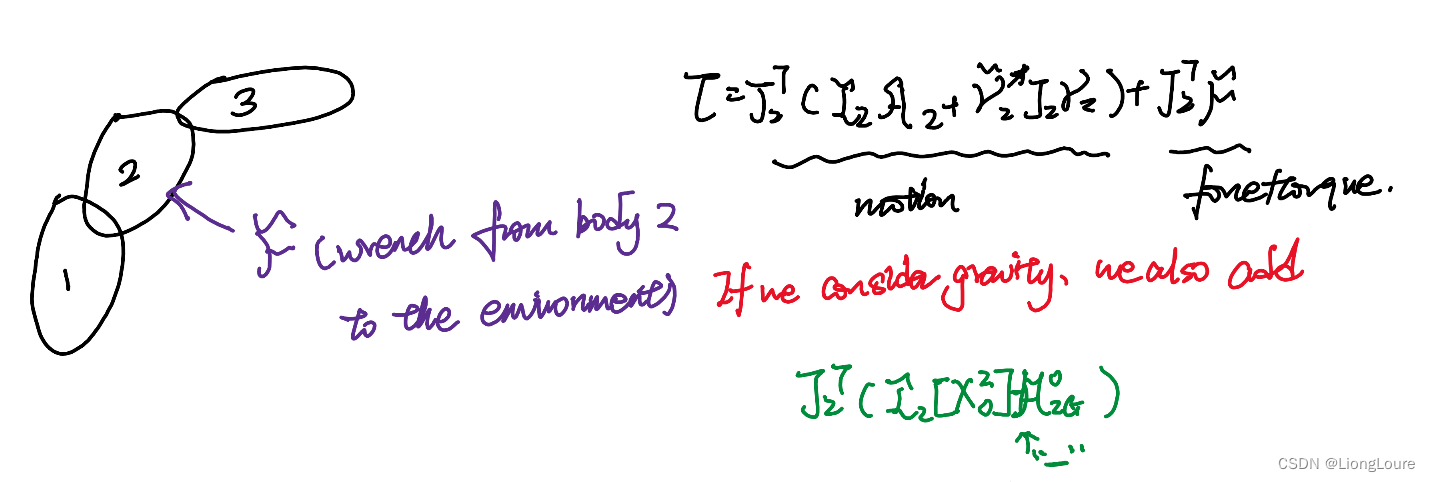
- Body 4:
F 4 + F G 4 = I 4 A 4 + V ~ 4 ∗ I 4 V 4 ⇒ F 4 = I 4 A 4 + V ~ 4 ∗ I 4 V 4 − F G 4 , F G 4 = I 4 A G 4 = I 4 [ X O 4 ] A G O \mathcal{F} _4+\mathcal{F} _{\mathrm{G}4}=\mathcal{I} _4\mathcal{A} _4+{\tilde{\mathcal{V}}_4}^*\mathcal{I} _4\mathcal{V} _4 \\ \Rightarrow \mathcal{F} _4=\mathcal{I} _4\mathcal{A} _4+{\tilde{\mathcal{V}}_4}^*\mathcal{I} _4\mathcal{V} _4-\mathcal{F} _{\mathrm{G}4},\mathcal{F} _{\mathrm{G}4}=\mathcal{I} _4\mathcal{A} _{\mathrm{G}}^{4}=\mathcal{I} _4\left[ X_{\mathrm{O}}^{4} \right] \mathcal{A} _{\mathrm{G}}^{O} F4+FG4=I4A4+V~4∗I4V4⇒F4=I4A4+V~4∗I4V4−FG4,FG4=I4AG4=I4[XO4]AGO
τ 4 = S 4 T F 4 \tau _4={\mathcal{S} _4}^{\mathrm{T}}\mathcal{F} _4 τ4=S4TF4 - Body 2:
F 2 = I 2 A 2 + V ~ 2 ∗ I 2 V 2 + F 4 + F 3 − F G 2 , F G 2 = I 2 [ X O 2 ] A G 2 O τ 2 = S 2 T F 2 \mathcal{F} _2=\mathcal{I} _2\mathcal{A} _2+{\tilde{\mathcal{V}}_2}^*\mathcal{I} _2\mathcal{V} _2+\mathcal{F} _4+\mathcal{F} _3-\mathcal{F} _{\mathrm{G}2},\mathcal{F} _{\mathrm{G}2}=\mathcal{I} _2\left[ X_{\mathrm{O}}^{2} \right] \mathcal{A} _{\mathrm{G}2}^{O} \\ \tau _2={\mathcal{S} _2}^{\mathrm{T}}\mathcal{F} _2 F2=I2A2+V~2∗I2V2+F4+F3−FG2,FG2=I2[XO2]AG2Oτ2=S2TF2
2.1.3 Recursive Newton-Euler Algorithm
τ ← R N E A ( θ , θ ˙ , θ ¨ , F e x t ; M o d e l ) \tau \gets RNEA\left( \theta ,\dot{\theta},\ddot{\theta},\mathcal{F} _{\mathrm{ext}};Model \right) τ←RNEA(θ,θ˙,θ¨,Fext;Model)
Initialize : V 0 = 0 , A 0 = − A G \mathcal{V} _0=0,\mathcal{A} _0=-\mathcal{A} _{\mathrm{G}} V0=0,A0=−AG (without gravity “trick” modify F i = I i A i + V ~ i ∗ I i V i − I i [ X O i ] A G i O \mathcal{F} _{\mathrm{i}}=\mathcal{I} _{\mathrm{i}}\mathcal{A} _{\mathrm{i}}+{\tilde{\mathcal{V}}_{\mathrm{i}}}^*\mathcal{I} _{\mathrm{i}}\mathcal{V} _{\mathrm{i}}-\mathcal{I} _{\mathrm{i}}\left[ X_{\mathrm{O}}^{i} \right] \mathcal{A} _{\mathrm{Gi}}^{O} Fi=IiAi+V~i∗IiVi−Ii[XOi]AGiO)
- Forward pass : For i = 1 i=1 i=1 to N N N
V i i = [ X p ( i ) i ] V p ( i ) p ( i ) + S i i θ ˙ i \mathcal{V} _{\mathrm{i}}^{i}=\left[ X_{\mathrm{p}\left( i \right)}^{i} \right] \mathcal{V} _{\mathrm{p}\left( i \right)}^{p\left( i \right)}+\mathcal{S} _{\mathrm{i}}^{i}\dot{\theta}_{\mathrm{i}} Vii=[Xp(i)i]Vp(i)p(i)+Siiθ˙i
A i i = [ X p ( i ) i ] A p ( i ) p ( i ) + V ~ i i S i i θ ˙ i + S i i θ ¨ i \mathcal{A} _{\mathrm{i}}^{i}=\left[ X_{\mathrm{p}\left( i \right)}^{i} \right] \mathcal{A} _{\mathrm{p}\left( i \right)}^{p\left( i \right)}+\tilde{\mathcal{V}}_{\mathrm{i}}^{i}\mathcal{S} _{\mathrm{i}}^{i}\dot{\theta}_{\mathrm{i}}+\mathcal{S} _{\mathrm{i}}^{i}\ddot{\theta}_{\mathrm{i}} Aii=[Xp(i)i]Ap(i)p(i)+V~iiSiiθ˙i+Siiθ¨i
F i = I i A i + V ~ i ∗ I i V i \mathcal{F} _{\mathrm{i}}=\mathcal{I} _{\mathrm{i}}\mathcal{A} _{\mathrm{i}}+{\tilde{\mathcal{V}}_{\mathrm{i}}}^*\mathcal{I} _{\mathrm{i}}\mathcal{V} _{\mathrm{i}} Fi=IiAi+V~i∗IiVi - Backward pass : For i = N i=N i=N to 1
τ i = S i T F i \tau _{\mathrm{i}}={\mathcal{S} _{\mathrm{i}}}^{\mathrm{T}}\mathcal{F} _{\mathrm{i}} τi=SiTFi
F p ( i ) = F p ( i ) + [ X i p ( i ) ] F i \mathcal{F} _{\mathrm{p}\left( i \right)}=\mathcal{F} _{\mathrm{p}\left( i \right)}+\left[ X_{\mathrm{i}}^{p\left( i \right)} \right] \mathcal{F} _{\mathrm{i}} Fp(i)=Fp(i)+[Xip(i)]Fi
3. Analytical Form of the Dynamics Model
3.1 Structures in Dynamic Equation
Jacobian of each link(body) : J 1 , ⋯ , J 4 J_1,\cdots ,J_4 J1,⋯,J4
J i J_{\mathrm{i}} Ji : denote the Jacobian of body(Link) i i i , i.e. V i = J i θ ˙ = [ J i 1 J i 2 J i 3 J i 4 ] [ θ ˙ 1 θ ˙ 2 θ ˙ 3 θ ˙ 4 ] \mathcal{V} _{\mathrm{i}}=J_{\mathrm{i}}\dot{\theta}=\left[ \begin{matrix} J_{\mathrm{i}1}& J_{\mathrm{i}2}& J_{\mathrm{i}3}& J_{\mathrm{i}4}\\ \end{matrix} \right] \left[ \begin{array}{c} \dot{\theta}_1\\ \dot{\theta}_2\\ \dot{\theta}_3\\ \dot{\theta}_4\\ \end{array} \right] Vi=Jiθ˙=[Ji1Ji2Ji3Ji4] θ˙1θ˙2θ˙3θ˙4
e.g. V 1 = J 1 θ ˙ = [ δ 11 S 1 δ 12 S 2 δ 13 S 3 δ 14 S 4 ] [ θ ˙ 1 θ ˙ 2 θ ˙ 3 θ ˙ 4 ] = [ S 1 0 0 0 ] [ θ ˙ 1 θ ˙ 2 θ ˙ 3 θ ˙ 4 ] δ i j = { 1 , i f j o i n t j s u p p o r t b o d y i 0 , o t h e r w i s e \mathcal{V} _1=J_1\dot{\theta}=\left[ \begin{matrix} \delta _{11}\mathcal{S} _1& \delta _{12}\mathcal{S} _2& \delta _{13}\mathcal{S} _3& \delta _{14}\mathcal{S} _4\\ \end{matrix} \right] \left[ \begin{array}{c} \dot{\theta}_1\\ \dot{\theta}_2\\ \dot{\theta}_3\\ \dot{\theta}_4\\ \end{array} \right] =\left[ \begin{matrix} \mathcal{S} _1& 0& 0& 0\\ \end{matrix} \right] \left[ \begin{array}{c} \dot{\theta}_1\\ \dot{\theta}_2\\ \dot{\theta}_3\\ \dot{\theta}_4\\ \end{array} \right] \\ \delta _{\mathrm{ij}}=\begin{cases} 1, if\,\,joint\,\,\mathrm{j} support\,\,body\,\,\mathrm{i}\\ 0, otherwise\\ \end{cases} V1=J1θ˙=[δ11S1δ12S2δ13S3δ14S4] θ˙1θ˙2θ˙3θ˙4 =[S1000] θ˙1θ˙2θ˙3θ˙4 δij={1,ifjointjsupportbodyi0,otherwise
V 2 = J 2 θ ˙ = [ S 1 S 2 0 0 ] θ ˙ ⇒ V 2 2 = [ [ X 1 2 ] S 2 1 S 2 2 0 0 ] θ ˙ \mathcal{V} _2=J_2\dot{\theta}=\left[ \begin{matrix} \mathcal{S} _1& \mathcal{S} _2& 0& 0\\ \end{matrix} \right] \dot{\theta}\Rightarrow \mathcal{V} _{2}^{2}=\left[ \left[ X_{1}^{2} \right] \begin{matrix} \mathcal{S} _{2}^{1}& \mathcal{S} _{2}^{2}& 0& 0\\ \end{matrix} \right] \dot{\theta} V2=J2θ˙=[S1S200]θ˙⇒V22=[[X12]S21S2200]θ˙
see the two-body example:
- Forward pass :
V 1 = S 1 θ ˙ 1 \mathcal{V} _1=\mathcal{S} _1\dot{\theta}_1 V1=S1θ˙1 , V 2 2 = [ [ X 1 2 ] S 2 1 S 2 2 ] [ θ ˙ 1 θ ˙ 2 ] \mathcal{V} _{2}^{2}=\left[ \begin{matrix} \left[ X_{1}^{2} \right] \mathcal{S} _{2}^{1}& \mathcal{S} _{2}^{2}\\ \end{matrix} \right] \left[ \begin{array}{c} \dot{\theta}_1\\ \dot{\theta}_2\\ \end{array} \right] V22=[[X12]S21S22][θ˙1θ˙2]
A 1 , A 2 \mathcal{A} _1, \mathcal{A} _2 A1,A2 - Backward pass :
F 2 = I 2 A 2 + V ~ 2 ∗ I 2 V 2 − F 2 e x t − F 2 G F 1 = I 1 A 1 + V ~ 1 ∗ I 1 V 1 − F 1 e x t − F 1 G + [ X 2 1 ] ( I 2 A 2 + V ~ 2 ∗ I 2 V 2 − F 2 e x t − F 2 G ) τ 2 = S 2 T F 2 τ 1 = S 1 T F 1 \mathcal{F} _2=\mathcal{I} _2\mathcal{A} _2+{\tilde{\mathcal{V}}_2}^*\mathcal{I} _2\mathcal{V} _2-\mathcal{F} _{2\mathrm{ext}}-\mathcal{F} _{2\mathrm{G}} \\ \mathcal{F} _1=\mathcal{I} _1\mathcal{A} _1+{\tilde{\mathcal{V}}_1}^*\mathcal{I} _1\mathcal{V} _1-\mathcal{F} _{1\mathrm{ext}}-\mathcal{F} _{1\mathrm{G}}+\left[ X_{2}^{1} \right] \left( \mathcal{I} _2\mathcal{A} _2+{\tilde{\mathcal{V}}_2}^*\mathcal{I} _2\mathcal{V} _2-\mathcal{F} _{2\mathrm{ext}}-\mathcal{F} _{2\mathrm{G}} \right) \\ \tau _2={\mathcal{S} _2}^{\mathrm{T}}\mathcal{F} _2 \\ \tau _1={\mathcal{S} _1}^{\mathrm{T}}\mathcal{F} _1 F2=I2A2+V~2∗I2V2−F2ext−F2GF1=I1A1+V~1∗I1V1−F1ext−F1G+[X21](I2A2+V~2∗I2V2−F2ext−F2G)τ2=S2TF2τ1=S1TF1
Overall torque expression :
τ 1 = S 1 T F 1 = S 1 T ( I 1 A 1 + V ~ 1 ∗ I 1 V 1 − F 1 e x t − F 1 G + [ X 2 1 ] ( I 2 A 2 + V ~ 2 ∗ I 2 V 2 − F 2 e x t − F 2 G ) ) = S 1 T ( I 1 A 1 + V ~ 1 ∗ I 1 V 1 ) + ( [ X 1 2 ] S 1 ) T ( I 2 A 2 + V ~ 2 ∗ I 2 V 2 ) − S 1 T ( F 1 e x t + F 1 G + [ X 2 1 ] ( F 2 e x t + F 2 G ) ) \tau _1={\mathcal{S} _1}^{\mathrm{T}}\mathcal{F} _1={\mathcal{S} _1}^{\mathrm{T}}\left( \mathcal{I} _1\mathcal{A} _1+{\tilde{\mathcal{V}}_1}^*\mathcal{I} _1\mathcal{V} _1-\mathcal{F} _{1\mathrm{ext}}-\mathcal{F} _{1\mathrm{G}}+\left[ X_{2}^{1} \right] \left( \mathcal{I} _2\mathcal{A} _2+{\tilde{\mathcal{V}}_2}^*\mathcal{I} _2\mathcal{V} _2-\mathcal{F} _{2\mathrm{ext}}-\mathcal{F} _{2\mathrm{G}} \right) \right) \\ ={\mathcal{S} _1}^{\mathrm{T}}\left( \mathcal{I} _1\mathcal{A} _1+{\tilde{\mathcal{V}}_1}^*\mathcal{I} _1\mathcal{V} _1 \right) +\left( \left[ X_{1}^{2} \right] \mathcal{S} _1 \right) ^{\mathrm{T}}\left( \mathcal{I} _2\mathcal{A} _2+{\tilde{\mathcal{V}}_2}^*\mathcal{I} _2\mathcal{V} _2 \right) -{\mathcal{S} _1}^{\mathrm{T}}\left( \mathcal{F} _{1\mathrm{ext}}+\mathcal{F} _{1\mathrm{G}}+\left[ X_{2}^{1} \right] \left( \mathcal{F} _{2\mathrm{ext}}+\mathcal{F} _{2\mathrm{G}} \right) \right) τ1=S1TF1=S1T(I1A1+V~1∗I1V1−F1ext−F1G+[X21](I2A2+V~2∗I2V2−F2ext−F2G))=S1T(I1A1+V~1∗I1V1)+([X12]S1)T(I2A2+V~2∗I2V2)−S1T(F1ext+F1G+[X21](F2ext+F2G))
due to motion of body 1 and 2 and external force of body 1 and 2
τ = [ τ 1 τ 2 ] = [ S 1 T ( I 1 A 1 + V ~ 1 ∗ I 1 V 1 ) + ( [ X 1 2 ] S 1 ) T ( I 2 A 2 + V ~ 2 ∗ I 2 V 2 ) − S 1 T ( F 1 e x t + F 1 G + [ X 2 1 ] ( F 2 e x t + F 2 G ) ) S 2 T ( I 2 A 2 + V ~ 2 ∗ I 2 V 2 − F 2 e x t − F 2 G ) ] = [ S 1 T 0 ] ( I 1 A 1 + V ~ 1 ∗ I 1 V 1 − F 1 e x t − F 1 G ) + [ ( [ X 1 2 ] S 1 ) T S 2 T ] ( I 2 A 2 + V ~ 2 ∗ I 2 V 2 − F 2 e x t − F 2 G ) = J 1 T ( I 1 A 1 + V ~ 1 ∗ I 1 V 1 − F 1 e x t − F 1 G ) + J 2 T ( I 2 A 2 + V ~ 2 ∗ I 2 V 2 − F 2 e x t − F 2 G ) \tau =\left[ \begin{array}{c} \tau _1\\ \tau _2\\ \end{array} \right] =\left[ \begin{array}{c} {\mathcal{S} _1}^{\mathrm{T}}\left( \mathcal{I} _1\mathcal{A} _1+{\tilde{\mathcal{V}}_1}^*\mathcal{I} _1\mathcal{V} _1 \right) +\left( \left[ X_{1}^{2} \right] \mathcal{S} _1 \right) ^{\mathrm{T}}\left( \mathcal{I} _2\mathcal{A} _2+{\tilde{\mathcal{V}}_2}^*\mathcal{I} _2\mathcal{V} _2 \right) -{\mathcal{S} _1}^{\mathrm{T}}\left( \mathcal{F} _{1\mathrm{ext}}+\mathcal{F} _{1\mathrm{G}}+\left[ X_{2}^{1} \right] \left( \mathcal{F} _{2\mathrm{ext}}+\mathcal{F} _{2\mathrm{G}} \right) \right)\\ {\mathcal{S} _2}^{\mathrm{T}}\left( \mathcal{I} _2\mathcal{A} _2+{\tilde{\mathcal{V}}_2}^*\mathcal{I} _2\mathcal{V} _2-\mathcal{F} _{2\mathrm{ext}}-\mathcal{F} _{2\mathrm{G}} \right)\\ \end{array} \right] \\ =\left[ \begin{array}{c} {\mathcal{S} _1}^{\mathrm{T}}\\ 0\\ \end{array} \right] \left( \mathcal{I} _1\mathcal{A} _1+{\tilde{\mathcal{V}}_1}^*\mathcal{I} _1\mathcal{V} _1-\mathcal{F} _{1\mathrm{ext}}-\mathcal{F} _{1\mathrm{G}} \right) +\left[ \begin{array}{c} \left( \left[ X_{1}^{2} \right] \mathcal{S} _1 \right) ^{\mathrm{T}}\\ {\mathcal{S} _2}^{\mathrm{T}}\\ \end{array} \right] \left( \mathcal{I} _2\mathcal{A} _2+{\tilde{\mathcal{V}}_2}^*\mathcal{I} _2\mathcal{V} _2-\mathcal{F} _{2\mathrm{ext}}-\mathcal{F} _{2\mathrm{G}} \right) \\ ={J_1}^{\mathrm{T}}\left( \mathcal{I} _1\mathcal{A} _1+{\tilde{\mathcal{V}}_1}^*\mathcal{I} _1\mathcal{V} _1-\mathcal{F} _{1\mathrm{ext}}-\mathcal{F} _{1\mathrm{G}} \right) +{J_2}^{\mathrm{T}}\left( \mathcal{I} _2\mathcal{A} _2+{\tilde{\mathcal{V}}_2}^*\mathcal{I} _2\mathcal{V} _2-\mathcal{F} _{2\mathrm{ext}}-\mathcal{F} _{2\mathrm{G}} \right) τ=[τ1τ2]= S1T(I1A1+V~1∗I1V1)+([X12]S1)T(I2A2+V~2∗I2V2)−S1T(F1ext+F1G+[X21](F2ext+F2G))S2T(I2A2+V~2∗I2V2−F2ext−F2G) =[S1T0](I1A1+V~1∗I1V1−F1ext−F1G)+[([X12]S1)TS2T](I2A2+V~2∗I2V2−F2ext−F2G)=J1T(I1A1+V~1∗I1V1−F1ext−F1G)+J2T(I2A2+V~2∗I2V2−F2ext−F2G)
Overall : in general with N-links / Joints
τ = ∑ i = 1 N J i T ( I i A i + V ~ i ∗ I i V i − F i e x t − F i G ) \tau =\sum_{i=1}^N{{J_{\mathrm{i}}}^{\mathrm{T}}\left( \mathcal{I} _{\mathrm{i}}\mathcal{A} _{\mathrm{i}}+{\tilde{\mathcal{V}}_{\mathrm{i}}}^*\mathcal{I} _{\mathrm{i}}\mathcal{V} _{\mathrm{i}}-\mathcal{F} _{\mathrm{iext}}-\mathcal{F} _{\mathrm{iG}} \right)} τ=i=1∑NJiT(IiAi+V~i∗IiVi−Fiext−FiG)
V i = J i θ ˙ A i = V ˙ i = ( J ˙ i θ ˙ + J i θ ¨ + V ~ i J i θ ˙ ) \mathcal{V} _{\mathrm{i}}=J_{\mathrm{i}}\dot{\theta} \\ \mathcal{A} _{\mathrm{i}}=\dot{\mathcal{V}}_{\mathrm{i}}=\left( \dot{J}_{\mathrm{i}}\dot{\theta}+J_{\mathrm{i}}\ddot{\theta}+\tilde{\mathcal{V}}_{\mathrm{i}}J_{\mathrm{i}}\dot{\theta} \right) Vi=Jiθ˙Ai=V˙i=(J˙iθ˙+Jiθ¨+V~iJiθ˙)
上式看上去难以理解,尤其是加速度旋量,本质上是因为在构件坐标系下的求导,相当于需要对运动基向量求导所产生的加速度
带入可得:
τ = ∑ i = 1 N J i T I i J i θ ¨ + ∑ i = 1 N J i T ( I i J ˙ i + I i V ~ i J i + V ~ i ∗ I i J i ) θ ˙ \tau =\sum_{i=1}^N{{J_{\mathrm{i}}}^{\mathrm{T}}\mathcal{I} _{\mathrm{i}}J_{\mathrm{i}}}\ddot{\theta}+\sum_{i=1}^N{{J_{\mathrm{i}}}^{\mathrm{T}}\left( \mathcal{I} _{\mathrm{i}}\dot{J}_{\mathrm{i}}+\mathcal{I} _{\mathrm{i}}\tilde{\mathcal{V}}_{\mathrm{i}}J_{\mathrm{i}}+{\tilde{\mathcal{V}}_{\mathrm{i}}}^*\mathcal{I} _{\mathrm{i}}J_{\mathrm{i}} \right)}\dot{\theta} τ=i=1∑NJiTIiJiθ¨+i=1∑NJiT(IiJ˙i+IiV~iJi+V~i∗IiJi)θ˙
∑ i = 1 N J i T I i J i = M ( θ ) , ∑ i = 1 N J i T ( I i J ˙ i + I i V ~ i J i + V ~ i ∗ I i J i ) = c ( θ , θ ˙ ) \sum_{i=1}^N{{J_{\mathrm{i}}}^{\mathrm{T}}\mathcal{I} _{\mathrm{i}}J_{\mathrm{i}}}=M\left( \theta \right) ,\sum_{i=1}^N{{J_{\mathrm{i}}}^{\mathrm{T}}\left( \mathcal{I} _{\mathrm{i}}\dot{J}_{\mathrm{i}}+\mathcal{I} _{\mathrm{i}}\tilde{\mathcal{V}}_{\mathrm{i}}J_{\mathrm{i}}+{\tilde{\mathcal{V}}_{\mathrm{i}}}^*\mathcal{I} _{\mathrm{i}}J_{\mathrm{i}} \right)}=c\left( \theta ,\dot{\theta} \right) ∑i=1NJiTIiJi=M(θ),∑i=1NJiT(IiJ˙i+IiV~iJi+V~i∗IiJi)=c(θ,θ˙) , τ G = ∑ i = 1 N J i T I i [ X O i ] ( − A i G O ) \tau _G=\sum_{i=1}^N{{J_{\mathrm{i}}}^{\mathrm{T}}\mathcal{I} _{\mathrm{i}}\left[ X_{\mathrm{O}}^{i} \right]}\left( -\mathcal{A} _{\mathrm{iG}}^{O} \right) τG=∑i=1NJiTIi[XOi](−AiGO)
最终理解: τ = M ( θ ) θ ¨ + c ( θ , θ ˙ ) θ ˙ + τ G + J T ( θ ) F e x t \tau =M\left( \theta \right) \ddot{\theta}+c\left( \theta ,\dot{\theta} \right) \dot{\theta}+\tau _G+J^{\mathrm{T}}\left( \theta \right) \mathcal{F} _{\mathrm{ext}} τ=M(θ)θ¨+c(θ,θ˙)θ˙+τG+JT(θ)Fext
F e x t \mathcal{F} _{\mathrm{ext}} Fext : applied from the body to environment
回顾:
J i J_{\mathrm{i}} Ji : body/link i Jacobian , V i ∣ 6 × 1 = J i ∣ 6 × n θ ˙ ∣ n × 1 \left. \mathcal{V} _{\mathrm{i}} \right|_{6\times 1}=\left. J_{\mathrm{i}} \right|_{6\times \mathrm{n}}\left. \dot{\theta} \right|_{\mathrm{n}\times 1} Vi∣6×1=Ji∣6×nθ˙ n×1
τ ∈ R n \tau \in \mathbb{R} ^n τ∈Rn , τ \tau τ play two major roles :
- generate motion
- generate force/torque
3.2 Properties of Dynamics Model of Multi-Body Systems
Only cpnsider body 2’s effect
4. Forward Dynamics Algorithms
4.1 Forward Dynamics Problem
τ = M ( θ ) θ ¨ + c ( θ , θ ˙ ) θ ˙ + τ G + J T ( θ ) F e x t = M ( θ ) θ ¨ + h ( θ , θ ˙ ) \tau =M\left( \theta \right) \ddot{\theta}+c\left( \theta ,\dot{\theta} \right) \dot{\theta}+\tau _G+J^{\mathrm{T}}\left( \theta \right) \mathcal{F} _{\mathrm{ext}}=M\left( \theta \right) \ddot{\theta}+h\left( \theta ,\dot{\theta} \right) τ=M(θ)θ¨+c(θ,θ˙)θ˙+τG+JT(θ)Fext=M(θ)θ¨+h(θ,θ˙)
-
Inverse dynamics : τ ← R N E A ( θ , θ ˙ , θ ¨ , F e x t ) \tau \gets RNEA\left( \theta ,\dot{\theta},\ddot{\theta},\mathcal{F} _{\mathrm{ext}} \right) τ←RNEA(θ,θ˙,θ¨,Fext) —— O ( N ) O\left( N \right) O(N) complexity
RNEA can work directly with a givenURDF-United Robotics Description Formatmodel (kinematic tree + joint model + dynamic parameters). It does not require explicit formula for M ( θ ) , h ( θ , θ ˙ ) M\left( \theta \right),h\left( \theta ,\dot{\theta} \right) M(θ),h(θ,θ˙) -
Forward dynamics : Given ( θ , θ ˙ ) , τ , F e x t \left( \theta ,\dot{\theta} \right) ,\tau ,\mathcal{F} _{\mathrm{ext}} (θ,θ˙),τ,Fext , find θ ¨ \ddot{\theta} θ¨
Calculate h ( θ , θ ˙ ) = c ( θ , θ ˙ ) θ ˙ + τ G + J T F e x t h\left( \theta ,\dot{\theta} \right) =c\left( \theta ,\dot{\theta} \right) \dot{\theta}+\tau _{\mathrm{G}}+J^{\mathrm{T}}\mathcal{F} _{\mathrm{ext}} h(θ,θ˙)=c(θ,θ˙)θ˙+τG+JTFext
Caculate mass matrix M ( θ ) = ∑ i = 1 N J i T I i J i M\left( \theta \right) =\sum_{i=1}^N{{J_{\mathrm{i}}}^{\mathrm{T}}\mathcal{I} _{\mathrm{i}}J_{\mathrm{i}}} M(θ)=∑i=1NJiTIiJi
Solve M θ ¨ = τ − h ⇒ θ ¨ = M − 1 ( τ − h ) M\ddot{\theta}=\tau -h\Rightarrow \ddot{\theta}=M^{-1}\left( \tau -h \right) Mθ¨=τ−h⇒θ¨=M−1(τ−h): This is not the most efficient way to find θ ¨ \ddot{\theta} θ¨
4.2 Caculations of h and M
Denote our inverse dynamics algorithm : τ = R N E A ( θ , θ ˙ , θ ¨ , F e x t ) = M θ ¨ + h \tau =RNEA\left( \theta ,\dot{\theta},\ddot{\theta},\mathcal{F} _{\mathrm{ext}} \right) =M\ddot{\theta}+h τ=RNEA(θ,θ˙,θ¨,Fext)=Mθ¨+h
-
Calculation of h h h : obviously , τ = h \tau =h τ=h if θ ¨ = 0 \ddot{\theta}=0 θ¨=0. Therefore, h h h can be computed via : h ( θ , θ ˙ ) = R N E A ( θ , θ ˙ , 0 , F e x t ) h\left( \theta ,\dot{\theta} \right) =RNEA\left( \theta ,\dot{\theta},0,\mathcal{F} _{\mathrm{ext}} \right) h(θ,θ˙)=RNEA(θ,θ˙,0,Fext)
-
Calculation of M M M : Note h ( θ , θ ˙ ) = c ( θ , θ ˙ ) θ ˙ + τ G + J T F e x t h\left( \theta ,\dot{\theta} \right) =c\left( \theta ,\dot{\theta} \right) \dot{\theta}+\tau _{\mathrm{G}}+J^{\mathrm{T}}\mathcal{F} _{\mathrm{ext}} h(θ,θ˙)=c(θ,θ˙)θ˙+τG+JTFext
Set G = 0 , F e x t = 0 , θ ˙ = 0 G=0,\mathcal{F} _{\mathrm{ext}}=0,\dot{\theta}=0 G=0,Fext=0,θ˙=0 , then h ( θ , θ ˙ ) = 0 h\left( \theta ,\dot{\theta} \right) =0 h(θ,θ˙)=0 , ⇒ τ = M ( θ ) θ ¨ \Rightarrow \tau =M\left( \theta \right) \ddot{\theta} ⇒τ=M(θ)θ¨
We can compute the j j jth colum of M ( θ ) M\left( \theta \right) M(θ) by calling the inverse algorithm
τ = M : , j ( θ ) = R N E A ( 0 , 0 , θ ¨ 0 , j , 0 ) \tau =M_{:,\mathrm{j}}\left( \theta \right) =RNEA\left( 0,0,\ddot{\theta}_{0,\mathrm{j}},0 \right) τ=M:,j(θ)=RNEA(0,0,θ¨0,j,0) , θ ¨ 0 , j \ddot{\theta}_{0,\mathrm{j}} θ¨0,j is a vector with all zeros except for a 1 at the j j jth entry
θ ¨ 0 , 1 = [ 1 0 ⋮ 0 ] , τ = [ M 1 ( θ ) ⋯ M n ( θ ) ] , M 1 , j ( θ ) = τ θ ¨ 0 , 1 \ddot{\theta}_{0,1}=\left[ \begin{array}{c} 1\\ 0\\ \vdots\\ 0\\ \end{array} \right] ,\tau =\left[ \begin{matrix} M_1\left( \theta \right)& \cdots& M_{\mathrm{n}}\left( \theta \right)\\ \end{matrix} \right] ,M_{1,\mathrm{j}}\left( \theta \right) =\tau \ddot{\theta}_{0,1} θ¨0,1= 10⋮0 ,τ=[M1(θ)⋯Mn(θ)],M1,j(θ)=τθ¨0,1 -
A more effiicient algorithm for computing M M M is the
Composite-Rigid-Body Algorithm(CRBA). Details can be found in Featherstone’s Book
4.3 Forward Dynamics Algorithms
Now assume we have θ , θ ˙ , τ , M ( θ ) , h \theta ,\dot{\theta},\tau ,M\left( \theta \right) ,h θ,θ˙,τ,M(θ),h , then we can immediately compute θ ¨ \ddot{\theta} θ¨ as θ ¨ = M − 1 ( τ − h ) \ddot{\theta}=M^{-1}\left( \tau -h \right) θ¨=M−1(τ−h) —— θ ¨ = F D ( τ , θ , θ ˙ , F e x t ) \ddot{\theta}=FD\left( \tau ,\theta ,\dot{\theta},\mathcal{F} _{\mathrm{ext}} \right) θ¨=FD(τ,θ,θ˙,Fext)
两种看似不同的求解思路,之间的关系是等同的
This provides a 2nd-order differential equation in R n \mathbb{R} ^n Rn , we can easily simulate the joint trajectory over any time period (under given ICs θ 0 , θ ˙ 0 \theta ^0,\dot{\theta}^0 θ0,θ˙0)
Computational Complexity:
RNEA : O ( N ) O\left( N \right) O(N)
h ( θ , θ ˙ ) = R N E A ( θ , θ ˙ , 0 , F e x t ) h\left( \theta ,\dot{\theta} \right) =RNEA\left( \theta ,\dot{\theta},0,\mathcal{F} _{\mathrm{ext}} \right) h(θ,θ˙)=RNEA(θ,θ˙,0,Fext) : O ( N ) O\left( N \right) O(N)
M ( θ ) M\left( \theta \right) M(θ) : O ( N 2 ) O\left( N^2 \right) O(N2)
M − 1 ( θ ) M^{-1}\left( \theta \right) M−1(θ) : O ( N 3 ) O\left( N^3 \right) O(N3)
Most efficient forward dynamics algorithm :
Articulate-Body Algorithm(ABA): O ( N ) O\left( N \right) O(N)
4.4 More Discussions
M ( θ ) M\left( \theta \right) M(θ) : Mass matrix , M T ( θ ) = M ( θ ) M^{\mathrm{T}}\left( \theta \right) =M\left( \theta \right) MT(θ)=M(θ), also positive semi-definite.
M ( θ ) = ∑ i = 1 N J i T I i J i M\left( \theta \right) =\sum_{i=1}^N{{J_{\mathrm{i}}}^{\mathrm{T}}\mathcal{I} _{\mathrm{i}}J_{\mathrm{i}}} M(θ)=∑i=1NJiTIiJi—— I i \mathcal{I} _{\mathrm{i}} Ii Inertia matrix symmetric / postive semi-definite
There are many equivalent ways to define c ( θ , θ ˙ ) c\left( \theta ,\dot{\theta} \right) c(θ,θ˙) , they are all related to the same product c ( θ , θ ˙ ) θ ˙ c\left( \theta ,\dot{\theta} \right) \dot{\theta} c(θ,θ˙)θ˙ —— common and confusing
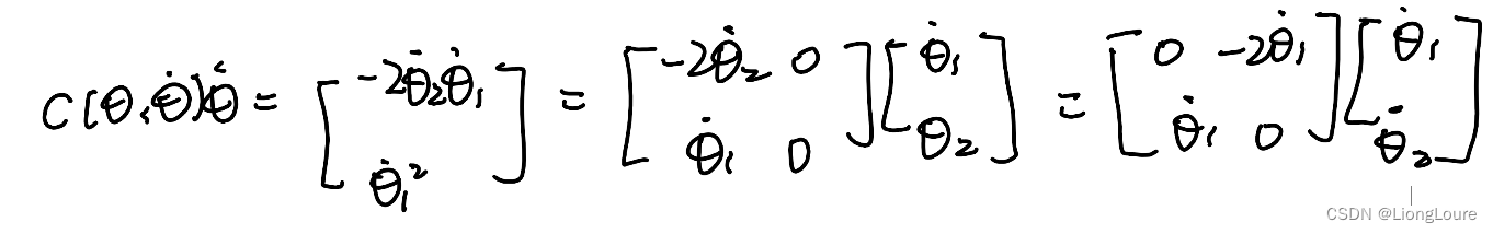
Typical expression for c c c : c i j = ∑ k = 1 1 2 ( ∂ M i j ∂ θ k + ∂ M i k ∂ θ j − ∂ M j k ∂ θ i ) θ ˙ k , Γ i j k = 1 2 ( ∂ M i j ∂ θ k + ∂ M i k ∂ θ j − ∂ M j k ∂ θ i ) c_{\mathrm{ij}}=\sum_{k=1}^{}{\frac{1}{2}\left( \frac{\partial M_{\mathrm{ij}}}{\partial \theta _{\mathrm{k}}}+\frac{\partial M_{\mathrm{ik}}}{\partial \theta _{\mathrm{j}}}-\frac{\partial M_{\mathrm{jk}}}{\partial \theta _{\mathrm{i}}} \right)}\dot{\theta}_{\mathrm{k}},\varGamma _{\mathrm{ijk}}=\frac{1}{2}\left( \frac{\partial M_{\mathrm{ij}}}{\partial \theta _{\mathrm{k}}}+\frac{\partial M_{\mathrm{ik}}}{\partial \theta _{\mathrm{j}}}-\frac{\partial M_{\mathrm{jk}}}{\partial \theta _{\mathrm{i}}} \right) cij=∑k=121(∂θk∂Mij+∂θj∂Mik−∂θi∂Mjk)θ˙k,Γijk=21(∂θk∂Mij+∂θj∂Mik−∂θi∂Mjk) chrostoffel symbol
c ( θ , θ ˙ ) c\left( \theta ,\dot{\theta} \right) c(θ,θ˙) defind using Γ i j k \varGamma _{\mathrm{ijk}} Γijk satisies : [ M ˙ − 2 c ] \left[ \dot{M}-2c \right] [M˙−2c] skew symmetric matrix ( n × n n\times n n×n)
M ( θ ) , c ( θ , θ ˙ ) , τ G M\left( \theta \right) ,c\left( \theta ,\dot{\theta} \right) ,\tau _G M(θ),c(θ,θ˙),τG all depend on I i \mathcal{I} _{\mathrm{i}} Ii linearly
相关文章:
[足式机器人]Part4 南科大高等机器人控制课 Ch09 Dynamics of Open Chains
本文仅供学习使用 本文参考: B站:CLEAR_LAB 笔者带更新-运动学 课程主讲教师: Prof. Wei Zhang 南科大高等机器人控制课 Ch09 Dynamics of Open Chains 1. Introduction1.1 From Single Rigid Body to Open Chains1.2 Preview of Open-Chain …...
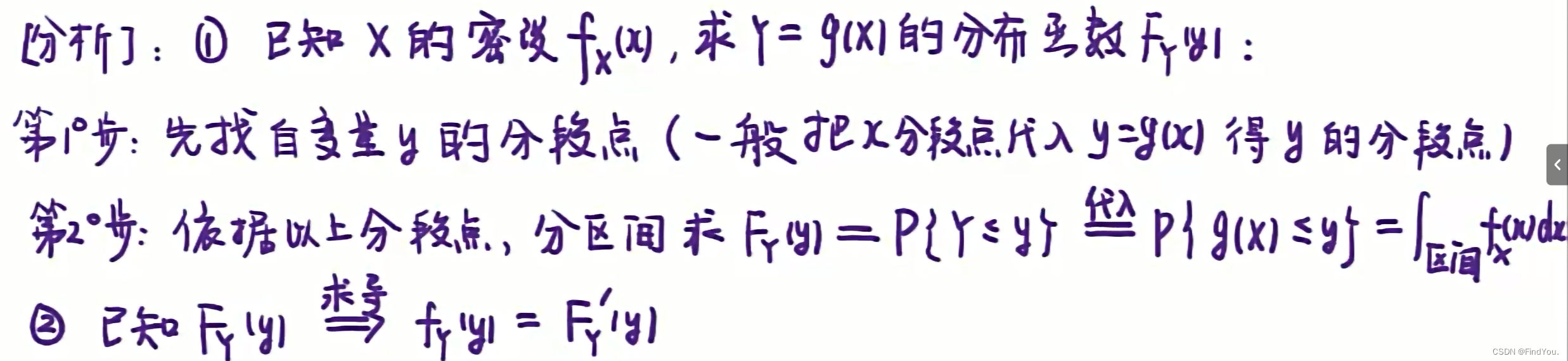
概率论复习
第一章:随机概率及其概率 A和B相容就是 AB 空集 全概率公式与贝叶斯公式: 伯努利求概率: 第二章:一维随机变量及其分布: 离散型随机变量求分布律: 利用常规离散性分布求概率: 连续性随机变量…...

ES客户端RestHighLevelClient的使用
1 RestHighLevelClient介绍 默认情况下,ElasticSearch使用两个端口来监听外部TCP流量。 9200端口:用于所有通过HTTP协议进行的API调用。包括搜索、聚合、监控、以及其他任何使用HTTP协议的请求。所有的客户端库都会使用该端口与ElasticSearch进行交互。…...

GitHub入门命令介绍
GitHub是当今最受欢迎的代码托管平台之一,它提供了强大的版本控制和协作功能。 对于初学者来说,熟悉GitHub的基本命令非常重要。下面介绍一些常用的GitHub命令。 一、安装Git 1. Windows系统:在Windows上使用GitHub之前,您需要先…...
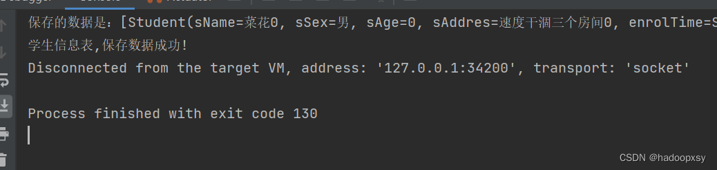
EasyExcel 简单导入
前边写过使用easyexcel进行简单、多sheet页的导出。今天周日利用空闲写一下对应简单的导入。 重点:springboot、easyExcel、桥接模式; 说明:本次使用实体类student:属性看前边章节内容; 1、公共导入service public …...

Termux搭建nodejs环境
安装nodejs ~ $ pkg install nodejs使用http-server搭建文件下载服务 先安 http-server 并启动 # 安装 http-server 包 ~ $ npm install -g http-server# 启动 http-server 服务 ~ $ http-server Starting up http-server, serving ./http-server version: 14.1.1http-serve…...
喜报丨迪捷软件入选2023年浙江省信息技术应用创新典型案例
12月6日,浙江省经信厅公示了2023年浙江省信息技术应用创新典型案例入围名单。本次案例征集活动,由浙江省经信厅、省密码管理局、工业和信息化部网络安全产业发展中心联合组织开展,共遴选出24个优秀典型解决方案,迪捷软件“基于全数…...
)
C语言连接zookeeper客户端(不能完全参考官网教程)
准备过程 1.通过VStudio 远程连接linux的开发环境; 2.g环境,通过MingW安装; 3.必须要安装好pthread.h的环境,不管是windows端(linux 可视化端开发就不管这个)还是linux端; 4.需要准备zookeeper…...

python排序
0. 背景 Python排序功能十分强大,可以进行基本排序或自定义排序。Python中提供两种不同的排序方法对各种各样的数据类型进行排序。 1. 使用sorted()函数排序 排序主要是对相同数据类型的元素进行的,包括数值和字符串两种数据类型。 1.1 对数值进行排…...
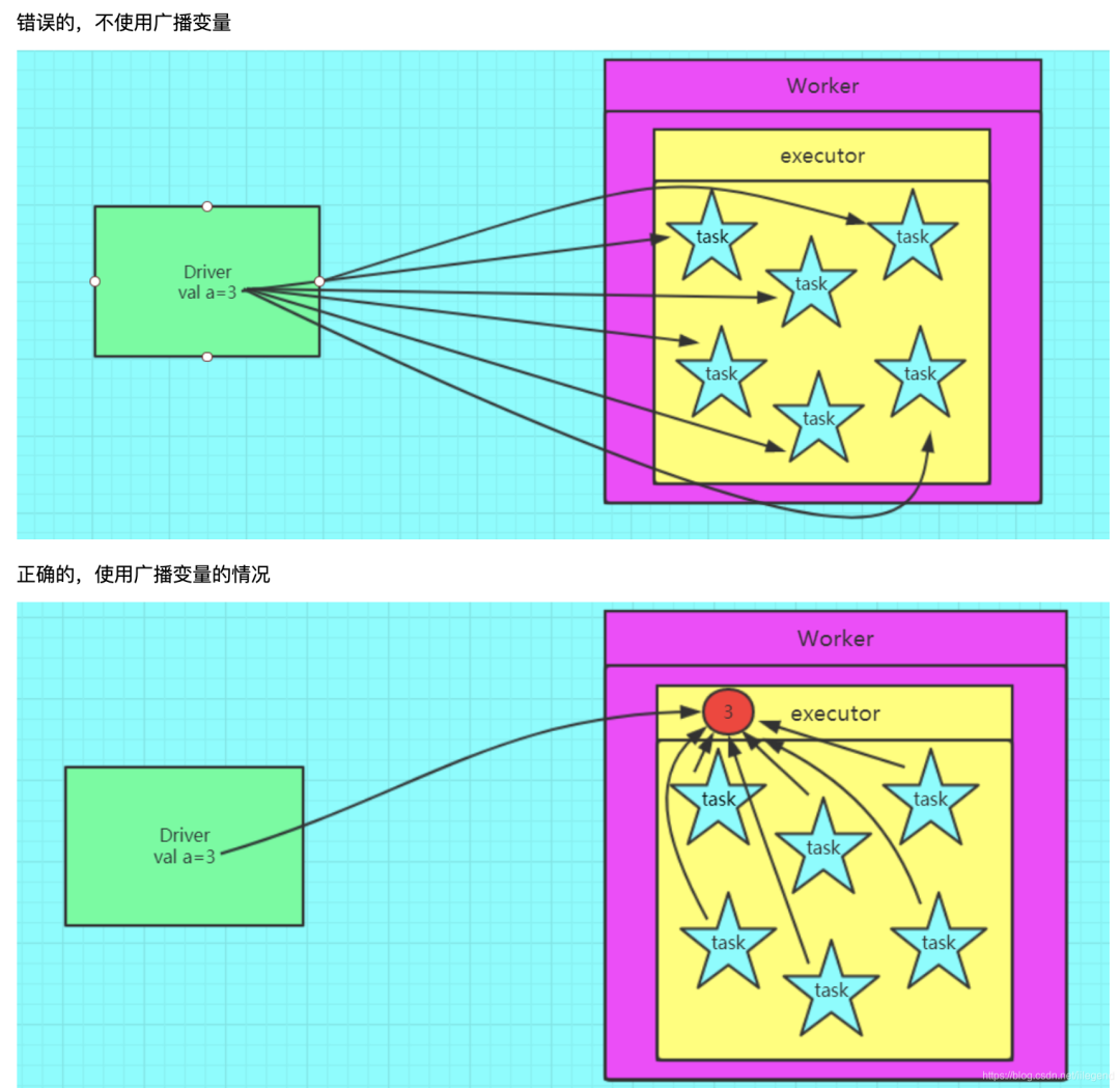
【Spark精讲】Spark Shuffle详解
目录 Shuffle概述 Shuffle执行流程 总体流程 中间文件 ShuffledRDD生成 Stage划分 Task划分 Map端写入(Shuffle Write) Reduce端读取(Shuffle Read) Spark Shuffle演变 SortShuffleManager运行机制 普通运行机制 bypass 运行机制 Tungsten Sort Shuffle 运行机制…...
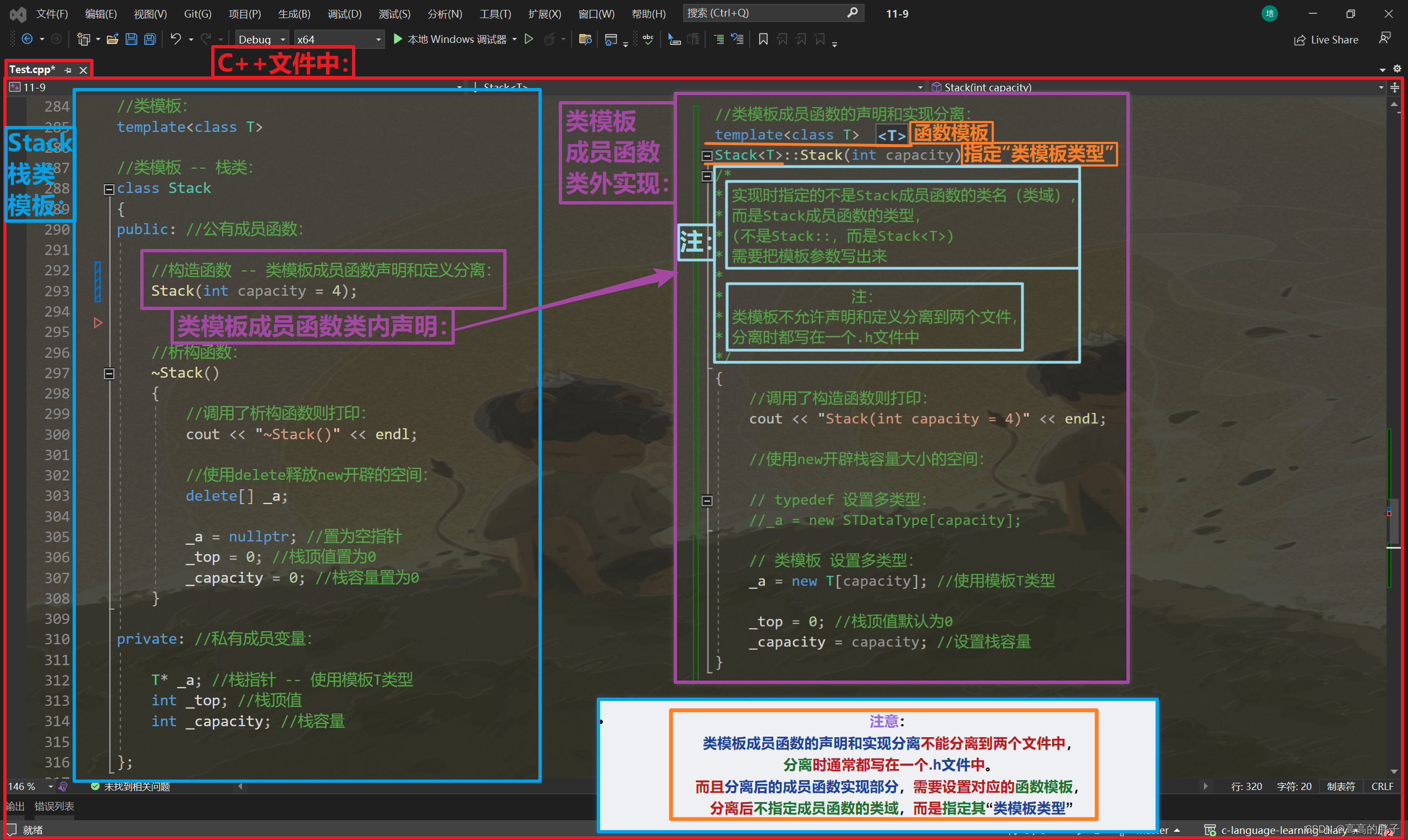
【C++初阶】八、初识模板(泛型编程、函数模板、类模板)
相关代码gitee自取: C语言学习日记: 加油努力 (gitee.com) 接上期: 【C初阶】七、内存管理 (C/C内存分布、C内存管理方式、operator new / delete 函数、定位new表达式) -CSDN博客 目录 一 . 泛型编程 二 . 函数模板 函数模板…...

珠海数字孪生赋能工业智能制造,助力制造业企业数字化转型
珠海数字孪生赋能工业智能制造,助力制造业企业数字化转型。数字孪生是利用物理模型、传感器更新及运行历史数据,集成多物理量、多尺度的仿真过程。巨蟹数科数字孪生通过构建物理车间与虚拟车间之间的有效映射并实时反馈机制,实现物理车间与虚…...
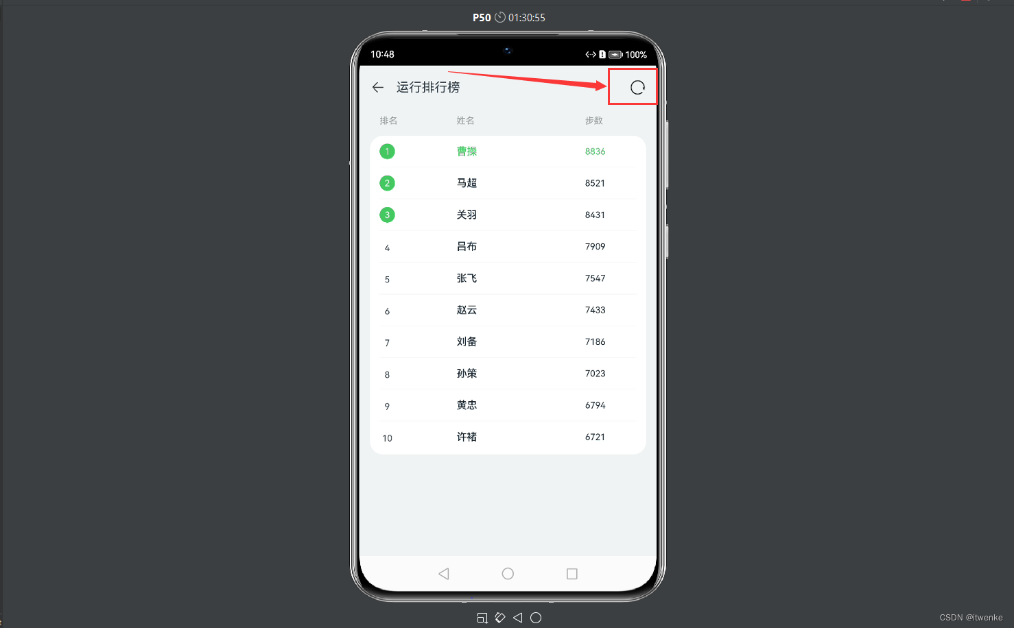
HarmonyOS开发实战:如何实现一个运动排名榜页面
HarmonyOS开发实战:如何实现一个运动排名榜页面 代码仓库: 运动排名榜页面 项目介绍 本项目使用声明式语法和组件化基础知识,搭建一个可刷新的排行榜页面。在排行榜页面中,使用循环渲染控制语法来实现列表数据渲染,…...

2019年第八届数学建模国际赛小美赛D题安全选举的答案是什么解题全过程文档及程序
2019年第八届数学建模国际赛小美赛 D题 安全选举的答案是什么 原题再现: 随着美国进入一场关键性的选举,在确保投票系统的完整性方面进展甚微。2016年总统大选期间,唐纳德特朗普因被指控受到外国干涉而入主白宫,这一问题再次成为…...
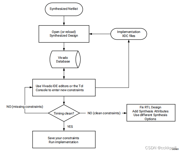
vivado 创建实施约束
创建实施约束 在您有了一个合成的网表之后,您可以将它与XDC文件一起加载到内存中,或者Tcl脚本已启用以进行实现。当加载XDC以便验证和更正任何不能应用的约束。在某些情况下,合成网表中的对象名称与精心设计。如果是这种情况,则必…...

【代码分析】MPI
代码解读 问题 model/AdaMPI.py:21 为什么下降分辨率model.CPN.unet.FeatMaskNetwork 为什么用的是mask,unet? MPI class MPIPredictor(nn.Module):def __init__(self,width384,height256,num_planes64,):super(MPIPredictor, self).__init__()self.…...
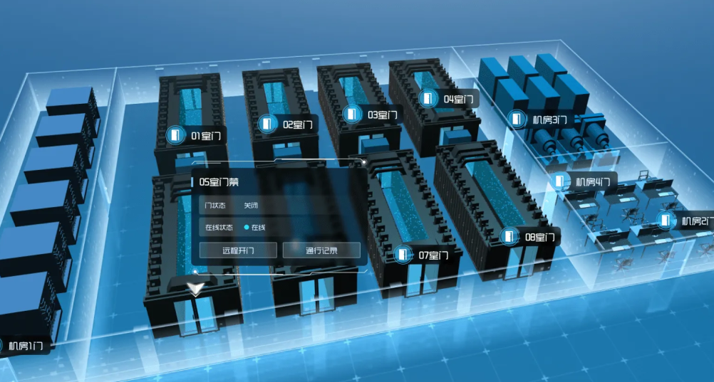
数字孪生Web3D智慧机房可视化运维云平台建设方案
前言 进入信息化时代,数字经济发展如火如荼,数据中心作为全行业数智化转型的智慧基座,重要性日益凸显。与此同时,随着东数西算工程落地和新型算力网络体系构建,数据中心建设规模和业务总量不断增长,机房管理…...

飞天使-docker知识点12-docker-compose
文章目录 docker-compose命令启动单个容器重启容器停止和启动容器停止和启动所有容器演示一个简单示范 docker-compose 部署有依赖问题 Docker Compose 是一个用于定义和运行多容器 Docker 应用程序的工具。它允许您使用简单的 YAML 文件来配置应用程序的服务、网络和存储等方…...
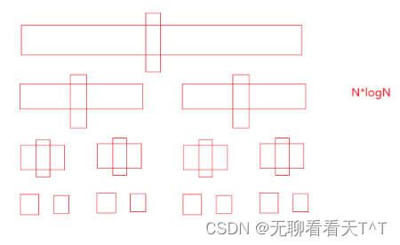
快速排序(一)
目录 快速排序(hoare版本) 初级实现 问题改进 中级实现 时空复杂度 高级实现 三数取中 快速排序(hoare版本) 历史背景:快速排序是Hoare于1962年提出的一种基于二叉树思想的交换排序方法 基本思想:…...
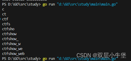
GO的sql注入盲注脚本
之间学习了go的语法 这里就开始go的爬虫 与其说是爬虫 其实就是网站的访问如何实现 因为之前想通过go写sql注入盲注脚本 发现不是那么简单 这里开始研究一下 首先是请求网站 这里貌似很简单 package mainimport ("fmt""net/http" )func main() {res, …...

终极KMS激活指南:如何免费激活Windows和Office的完整教程
终极KMS激活指南:如何免费激活Windows和Office的完整教程 【免费下载链接】KMS_VL_ALL_AIO Smart Activation Script 项目地址: https://gitcode.com/gh_mirrors/km/KMS_VL_ALL_AIO 还在为Windows和Office的激活问题烦恼吗?KMS_VL_ALL_AIO是一款开…...

别再手动算位宽了!Vivado FIR IP核的位宽计算逻辑与配置避坑指南
Vivado FIR IP核位宽计算实战:从黑盒解析到精准配置 在FPGA数字信号处理领域,FIR滤波器作为基础构建模块,其性能表现直接影响整个系统的信号处理质量。而位宽配置这个看似简单的参数,往往成为项目后期调试阶段的"隐形杀手&qu…...

OpenCore Legacy Patcher终极指南:让老Mac免费运行最新macOS的完整教程
OpenCore Legacy Patcher终极指南:让老Mac免费运行最新macOS的完整教程 【免费下载链接】OpenCore-Legacy-Patcher Experience macOS just like before 项目地址: https://gitcode.com/GitHub_Trending/op/OpenCore-Legacy-Patcher OpenCore Legacy Patcher是…...

UEFITool终极指南:轻松解析和编辑UEFI固件的开源利器
UEFITool终极指南:轻松解析和编辑UEFI固件的开源利器 【免费下载链接】UEFITool UEFI firmware image viewer and editor 项目地址: https://gitcode.com/gh_mirrors/ue/UEFITool 你是否曾好奇计算机启动时底层发生了什么?想要深入了解UEFI固件的…...

3个维度深度解析:UABEA如何重塑Unity资源处理生态
3个维度深度解析:UABEA如何重塑Unity资源处理生态 【免费下载链接】UABEA c# uabe for newer versions of unity 项目地址: https://gitcode.com/gh_mirrors/ua/UABEA 在Unity游戏开发和资源处理的复杂生态中,开发者常常面临一个核心挑战…...
.name()到可读类型名)
C++运行时类型识别实战:从typeid().name()到可读类型名
1. 为什么我们需要关心运行时类型识别? 在C开发中,我们经常会遇到需要知道某个变量或表达式具体类型的情况。特别是在调试复杂代码、编写泛型程序或进行元编程时,能够准确获取类型信息就显得尤为重要。想象一下,当你看到一个日志输…...

基于Rust与Candle的AI推理引擎cria:简化大模型本地部署与优化
1. 项目概述:从“左移”到“创造”的AI推理引擎 最近在折腾AI模型本地部署和推理优化的朋友,可能都绕不开一个名字: cria 。这个由 leftmove 开源的项目,全称是“Cria: The AI Inference Engine”,直译过来就是“创…...

Nixtla时间序列预测库实战:从统计模型到深度学习的一站式解决方案
1. 项目概述:时间序列预测的“瑞士军刀”如果你正在处理销售预测、服务器负载监控或者任何与时间相关的数据预测问题,并且厌倦了在复杂的模型库和繁琐的预处理步骤之间反复横跳,那么 Nixtla 这个开源项目很可能就是你一直在找的“瑞士军刀”。…...

认识Python数据包套接字
如你所知,数据包格式套接字(Datagram Sockets)也叫“无连接的套接字”,在代码中使用 SOCK_DGRAM 表示。可以将 SOCK_DGRAM 比喻成高速移动的摩托车快递,它有以下特征:强调快速传输而非传输顺序;…...

三维重建下半场,拼的全是底层基建实力!
三维重建已从算法创新竞赛正式迈入基础设施比拼新阶段,主流技术路线逐步收敛,单纯算法红利见顶,行业竞争核心转向数据、算力、平台、生态等底层综合能力。当下竞争不再只比模型效果,而是聚焦四大核心基建维度:采集传感…...