K-近邻和神经网络
K-近邻(K-NN, K-Nearest Neighbors)
原理
K-近邻(K-NN)是一种非参数分类和回归算法。K-NN 的主要思想是根据距离度量(如欧氏距离)找到训练数据集中与待预测样本最近的 K 个样本,并根据这 K 个样本的标签来进行预测。对于分类任务,K-NN 通过投票的方式选择出现最多的类别作为预测结果;对于回归任务,K-NN 通过计算 K 个最近邻样本的平均值来进行预测。
公式
K-NN 的主要步骤包括:
- 计算待预测样本与训练集中每个样本之间的距离。常用的距离度量包括欧氏距离、曼哈顿距离等。

- 找到距离最近的 K 个样本。
- 对于分类任务,通过投票决定预测结果:

其中,Nk 表示样本 x 的 K 个最近邻样本集合,I 是指示函数。
- 对于回归任务,通过计算平均值决定预测结果:

生活场景应用的案例
手写数字识别:K-NN 可以用于手写数字识别任务。假设我们有一个手写数字的图片数据集,每张图片都被标注了对应的数字。我们可以使用 K-NN 模型来识别新图片中的数字。
案例描述
假设我们有一个手写数字图片的数据集,包括以下特征:
- 图片像素值(每张图片由一个固定大小的像素矩阵表示)
我们希望通过这些像素值来预测图片中的数字。我们可以使用 K-NN 模型进行训练和预测。训练完成后,我们可以使用模型来识别新图片中的数字,并评估模型的性能。
代码解析
下面是一个使用 Python 实现上述手写数字识别案例的示例,使用了 scikit-learn 库。
import numpy as np
import pandas as pd
from sklearn.model_selection import train_test_split
from sklearn.neighbors import KNeighborsClassifier
from sklearn.metrics import accuracy_score, confusion_matrix, classification_report
import matplotlib.pyplot as plt
from sklearn.datasets import load_digits# 载入手写数字数据集
digits = load_digits()
X = digits.data
y = digits.target# 拆分训练集和测试集
X_train, X_test, y_train, y_test = train_test_split(X, y, test_size=0.2, random_state=42)# 创建K-NN模型并训练
k = 5
model = KNeighborsClassifier(n_neighbors=k)
model.fit(X_train, y_train)# 预测
y_pred = model.predict(X_test)# 评估模型
accuracy = accuracy_score(y_test, y_pred)
cm = confusion_matrix(y_test, y_pred)
report = classification_report(y_test, y_pred)print(f"Accuracy: {accuracy}")
print("Confusion Matrix:")
print(cm)
print("Classification Report:")
print(report)# 可视化部分测试结果
fig, axes = plt.subplots(1, 5, figsize=(10, 3))
for ax, image, prediction in zip(axes, X_test, y_pred):ax.set_axis_off()image = image.reshape(8, 8)ax.imshow(image, cmap=plt.cm.gray_r, interpolation='nearest')ax.set_title(f'Pred: {prediction}')
plt.show()
在这个示例中:
- 我们使用了
sklearn.datasets中的手写数字数据集。这个数据集包含了 8x8 像素的图片,每张图片代表一个手写数字。 - 将数据集拆分为训练集和测试集。
- 使用训练集训练 K-NN 分类模型。
- 通过测试集进行预测并评估模型的性能。
- 输出准确率(accuracy)、混淆矩阵(confusion matrix)和分类报告(classification report)。
- 可视化部分测试结果,展示模型的预测效果。
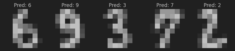
这个案例展示了如何使用 K-NN 模型来识别手写数字,基于图片的像素值特征。模型训练完成后,可以用于预测新图片中的数字,并帮助解决实际的手写数字识别问题。
神经网络(Neural Network)
原理
神经网络是一种模仿生物神经元结构的计算模型,由多个节点(神经元)和连接(权重)组成。神经网络主要由输入层、隐藏层和输出层构成,每一层包含若干神经元。通过层与层之间的连接和激活函数(如ReLU、Sigmoid等),神经网络能够拟合复杂的非线性关系,实现分类、回归等任务。
训练神经网络的过程通常使用反向传播算法,通过计算损失函数的梯度来调整网络的权重,以最小化预测误差。
公式
- 神经元的线性组合:

其中,xi 是输入,wi 是权重,b 是偏置,z 是神经元的加权和。
- 激活函数: 常用的激活函数包括:
- Sigmoid 函数:

- ReLU 函数:

- 反向传播:
反向传播算法通过计算损失函数的梯度来更新权重:

其中,η 是学习率,L 是损失函数。
生活场景应用的案例
图像分类:神经网络广泛应用于图像分类任务。假设我们有一个包含手写数字图片的数据集,每张图片都被标注了对应的数字。我们可以使用神经网络模型来识别新图片中的数字。
案例描述
假设我们有一个手写数字图片的数据集,包括以下特征:
- 图片像素值(每张图片由一个固定大小的像素矩阵表示)
我们希望通过这些像素值来预测图片中的数字。我们可以使用神经网络模型进行训练和预测。训练完成后,我们可以使用模型来识别新图片中的数字,并评估模型的性能。
代码解析
下面是一个使用 Python 实现上述手写数字识别案例的示例,使用了 tensorflow 和 keras 库。
import numpy as np
import pandas as pd
from sklearn.model_selection import train_test_split
from sklearn.metrics import classification_report
import matplotlib.pyplot as plt
import tensorflow as tf
from tensorflow.keras.models import Sequential
from tensorflow.keras.layers import Dense, Flatten
from tensorflow.keras.utils import to_categorical
from sklearn.datasets import load_digits# 载入手写数字数据集
digits = load_digits()
X = digits.images
y = digits.target# 预处理数据
X = X / 16.0  # 将像素值归一化到 [0, 1]
y = to_categorical(y, num_classes=10)  # 将标签转换为one-hot编码# 调整数据维度以适应TensorFlow模型
X = X.reshape(-1, 8, 8, 1)  # 使用-1使reshape自动计算样本数量# 拆分训练集和测试集
X_train, X_test, y_train, y_test = train_test_split(X, y, test_size=0.2, random_state=42)# 创建神经网络模型
model = Sequential([Flatten(input_shape=(8, 8, 1)),  # 展平输入图像Dense(128, activation='relu'),  # 隐藏层,包含128个神经元Dense(64, activation='relu'),  # 隐藏层,包含64个神经元Dense(10, activation='softmax')  # 输出层,包含10个神经元,对应10个类别
])# 编译模型
model.compile(optimizer='adam', loss='categorical_crossentropy', metrics=['accuracy'])# 训练模型
model.fit(X_train, y_train, epochs=20, batch_size=32, validation_split=0.2)# 评估模型
loss, accuracy = model.evaluate(X_test, y_test)
y_pred = model.predict(X_test)
y_pred_classes = np.argmax(y_pred, axis=1)
y_true = np.argmax(y_test, axis=1)print(f"Accuracy: {accuracy}")
print("Classification Report:")
print(classification_report(y_true, y_pred_classes))# 可视化部分测试结果
fig, axes = plt.subplots(1, 5, figsize=(10, 3))
for ax, image, prediction in zip(axes, X_test, y_pred_classes):ax.set_axis_off()image = image.reshape(8, 8)  # 确保图像形状正确ax.imshow(image, cmap=plt.cm.gray_r, interpolation='nearest')ax.set_title(f'Pred: {prediction}')
plt.show()
在这个示例中:
- 我们使用了
sklearn.datasets中的手写数字数据集。这个数据集包含了 8x8 像素的图片,每张图片代表一个手写数字。 - 将数据集拆分为训练集和测试集,并对数据进行预处理,将像素值归一化并将标签转换为 one-hot 编码。
- 创建了一个包含两个隐藏层的神经网络模型。
- 使用训练集训练神经网络模型。
- 通过测试集进行预测并评估模型的性能。
- 输出准确率(accuracy)和分类报告(classification report)。
- 可视化部分测试结果,展示模型的预测效果。

这个案例展示了如何使用神经网络模型来识别手写数字,基于图片的像素值特征。模型训练完成后,可以用于预测新图片中的数字,并帮助解决实际的手写数字识别问题。
具体应用
- 对预测结果进行可视化展示:
-
- 在预测结果后,展示原始图片及其预测结果。
- 保存和加载训练好的模型:
-
- 保存训练好的模型。
- 加载已保存的模型进行预测。
import os
import numpy as np
import pandas as pd
from sklearn.model_selection import train_test_split
from sklearn.metrics import classification_report
import matplotlib.pyplot as plt
import tensorflow as tf
from tensorflow.keras.models import Sequential, load_model
from tensorflow.keras.layers import Dense, Flatten
from tensorflow.keras.utils import to_categorical
from sklearn.datasets import load_digits
from PIL import Image  # 用于加载自定义图片# 载入手写数字数据集
digits = load_digits()
X = digits.images
y = digits.target# 预处理数据
X = X / 16.0  # 将像素值归一化到 [0, 1]
y = to_categorical(y, num_classes=10)  # 将标签转换为one-hot编码# 调整数据维度以适应TensorFlow模型
X = X.reshape(-1, 8, 8, 1)  # 使用-1使reshape自动计算样本数量# 拆分训练集和测试集
X_train, X_test, y_train, y_test = train_test_split(X, y, test_size=0.2, random_state=42)# 创建神经网络模型
model = Sequential([Flatten(input_shape=(8, 8, 1)),  # 展平输入图像Dense(128, activation='relu'),  # 隐藏层,包含128个神经元Dense(64, activation='relu'),  # 隐藏层,包含64个神经元Dense(10, activation='softmax')  # 输出层,包含10个神经元,对应10个类别
])# 编译模型
model.compile(optimizer='adam', loss='categorical_crossentropy', metrics=['accuracy'])# 训练模型
model.fit(X_train, y_train, epochs=20, batch_size=32, validation_split=0.2)# 保存训练好的模型
model.save('digit_recognition_model.h5')# 加载训练好的模型
# model = load_model('digit_recognition_model.h5')# 评估模型
loss, accuracy = model.evaluate(X_test, y_test)
y_pred = model.predict(X_test)
y_pred_classes = np.argmax(y_pred, axis=1)
y_true = np.argmax(y_test, axis=1)print(f"Accuracy: {accuracy}")
print("Classification Report:")
print(classification_report(y_true, y_pred_classes))# 可视化部分测试结果
fig, axes = plt.subplots(1, 5, figsize=(10, 3))
for ax, image, prediction in zip(axes, X_test, y_pred_classes):ax.set_axis_off()image = image.reshape(8, 8)  # 确保图像形状正确ax.imshow(image, cmap=plt.cm.gray_r, interpolation='nearest')ax.set_title(f'Pred: {prediction}')
plt.show()# 加载并预处理单张图片
def load_and_preprocess_image(filepath):img = Image.open(filepath).convert('L')  # 转换为灰度图像img = img.resize((8, 8))  # 调整图像大小为8x8img = np.array(img) / 16.0  # 归一化像素值img = img.reshape(1, 8, 8, 1)  # 调整图像维度return img# 加载并预处理文件夹中的所有图片
def load_images_from_folder(folder):images = []filepaths = []for filename in os.listdir(folder):if filename.endswith(('png', 'jpg', 'jpeg')):filepath = os.path.join(folder, filename)img = load_and_preprocess_image(filepath)images.append(img)filepaths.append(filepath)return np.vstack(images), filepaths# 使用模型预测文件夹中的多张图片
def predict_custom_images_from_folder(folder):imgs, filepaths = load_images_from_folder(folder)preds = model.predict(imgs)pred_classes = np.argmax(preds, axis=1)return pred_classes, filepaths# 示例:预测文件夹中的多张自定义图片并展示结果
custom_image_folder = 'path/to/your/folder'  # 替换为自定义图片文件夹路径
predicted_classes, filepaths = predict_custom_images_from_folder(custom_image_folder)# 打印预测结果并可视化
fig, axes = plt.subplots(1, len(filepaths), figsize=(15, 3))
for ax, filepath, pred_class in zip(axes, filepaths, predicted_classes):ax.set_axis_off()img = Image.open(filepath).convert('L')img = img.resize((8, 8))img = np.array(imgax.imshow(img, cmap=plt.cm.gray_r, interpolation='nearest')ax.set_title(f'Pred: {pred_class}')print(f'The predicted class for {filepath} is: {pred_class}')
plt.show()
a. 添加更多的训练数据来提高模型的准确性。
b. 使用混淆矩阵来详细分析模型的分类结果。
import os
import numpy as np
import pandas as pd
from sklearn.model_selection import train_test_split
from sklearn.metrics import classification_report, confusion_matrix, ConfusionMatrixDisplay
import matplotlib.pyplot as plt
import tensorflow as tf
from tensorflow.keras.models import Sequential, load_model
from tensorflow.keras.layers import Dense, Flatten
from tensorflow.keras.utils import to_categorical
from tensorflow.keras.preprocessing.image import ImageDataGenerator
from sklearn.datasets import load_digits
from PIL import Image# 载入手写数字数据集
digits = load_digits()
X = digits.images
y = digits.target# 预处理数据
X = X / 16.0  # 将像素值归一化到 [0, 1]
y = to_categorical(y, num_classes=10)  # 将标签转换为one-hot编码# 调整数据维度以适应TensorFlow模型
X = X.reshape(-1, 8, 8, 1)  # 使用-1使reshape自动计算样本数量# 拆分训练集和测试集
X_train, X_test, y_train, y_test = train_test_split(X, y, test_size=0.2, random_state=42)# 再拆分训练集以创建验证集
X_train, X_val, y_train, y_val = train_test_split(X_train, y_train, test_size=0.2, random_state=42)# 数据扩充
datagen = ImageDataGenerator(rotation_range=10,zoom_range=0.1,width_shift_range=0.1,height_shift_range=0.1
)
datagen.fit(X_train)# 创建神经网络模型
model = Sequential([Flatten(input_shape=(8, 8, 1)),  # 展平输入图像Dense(128, activation='relu'),  # 隐藏层,包含128个神经元Dense(64, activation='relu'),  # 隐藏层,包含64个神经元Dense(10, activation='softmax')  # 输出层,包含10个神经元,对应10个类别
])# 编译模型
model.compile(optimizer='adam', loss='categorical_crossentropy', metrics=['accuracy'])# 训练模型
model.fit(datagen.flow(X_train, y_train, batch_size=32), epochs=20, validation_data=(X_val, y_val))# 保存训练好的模型
model.save('digit_recognition_model.h5')# 加载训练好的模型
# model = load_model('digit_recognition_model.h5')# 评估模型
loss, accuracy = model.evaluate(X_test, y_test)
y_pred = model.predict(X_test)
y_pred_classes = np.argmax(y_pred, axis=1)
y_true = np.argmax(y_test, axis=1)print(f"Accuracy: {accuracy}")
print("Classification Report:")
print(classification_report(y_true, y_pred_classes))# 生成混淆矩阵
cm = confusion_matrix(y_true, y_pred_classes)
disp = ConfusionMatrixDisplay(confusion_matrix=cm, display_labels=np.arange(10))
disp.plot(cmap=plt.cm.Blues)
plt.show()# 可视化部分测试结果
fig, axes = plt.subplots(1, 5, figsize=(10, 3))
for ax, image, prediction in zip(axes, X_test, y_pred_classes):ax.set_axis_off()image = image.reshape(8, 8)  # 确保图像形状正确ax.imshow(image, cmap=plt.cm.gray_r, interpolation='nearest')ax.set_title(f'Pred: {prediction}')
plt.show()# 加载并预处理单张图片
def load_and_preprocess_image(filepath):img = Image.open(filepath).convert('L')  # 转换为灰度图像img = img.resize((8, 8))  # 调整图像大小为8x8img = np.array(img) / 16.0  # 归一化像素值img = img.reshape(1, 8, 8, 1)  # 调整图像维度return img# 加载并预处理文件夹中的所有图片
def load_images_from_folder(folder):images = []filepaths = []for filename in os.listdir(folder):if filename.endswith(('png', 'jpg', 'jpeg')):filepath = os.path.join(folder, filename)img = load_and_preprocess_image(filepath)images.append(img)filepaths.append(filepath)return np.vstack(images), filepaths# 使用模型预测文件夹中的多张图片
def predict_custom_images_from_folder(folder):imgs, filepaths = load_images_from_folder(folder)preds = model.predict(imgs)pred_classes = np.argmax(preds, axis=1)return pred_classes, filepaths# 示例:预测文件夹中的多张自定义图片并展示结果
custom_image_folder = 'path/to/your/folder'  # 替换为自定义图片文件夹路径
predicted_classes, filepaths = predict_custom_images_from_folder(custom_image_folder)# 打印预测结果并可视化
fig, axes = plt.subplots(1, len(filepaths), figsize=(15, 3))
for ax, filepath, pred_class in zip(axes, filepaths, predicted_classes):ax.set_axis_off()img = Image.open(filepath).convert('L')img = img.resize((8, 8))img = np.array(img)ax.imshow(img, cmap=plt.cm.gray_r, interpolation='nearest')ax.set_title(f'Pred: {pred_class}')print(f'The predicted class for {filepath} is: {pred_class}')
plt.show()
a. 使用更多的手写数字样本进行训练,以提高模型对手写数字的识别能力。
b. 尝试使用不同的模型架构,如卷积神经网络(CNN),以提高模型的识别准确率。
import os
import numpy as np
import pandas as pd
from sklearn.model_selection import train_test_split
from sklearn.metrics import classification_report, confusion_matrix, ConfusionMatrixDisplay
import matplotlib.pyplot as plt
import tensorflow as tf
from tensorflow.keras.models import Sequential, load_model
from tensorflow.keras.layers import Dense, Flatten
from tensorflow.keras.utils import to_categorical
from tensorflow.keras.preprocessing.image import ImageDataGenerator
from sklearn.datasets import load_digits
from PIL import Image# 载入手写数字数据集
digits = load_digits()
X = digits.images
y = digits.target# 预处理数据
X = X / 16.0  # 将像素值归一化到 [0, 1]
y = to_categorical(y, num_classes=10)  # 将标签转换为one-hot编码# 调整数据维度以适应TensorFlow模型
X = X.reshape(-1, 8, 8, 1)  # 使用-1使reshape自动计算样本数量# 拆分训练集和测试集
X_train, X_test, y_train, y_test = train_test_split(X, y, test_size=0.2, random_state=42)# 再拆分训练集以创建验证集
X_train, X_val, y_train, y_val = train_test_split(X_train, y_train, test_size=0.2, random_state=42)# 数据扩充
datagen = ImageDataGenerator(rotation_range=5,zoom_range=0.05,width_shift_range=0.05,height_shift_range=0.05
)
datagen.fit(X_train)# 创建神经网络模型
model = Sequential([Flatten(input_shape=(8, 8, 1)),  # 展平输入图像Dense(128, activation='relu'),  # 隐藏层,包含128个神经元Dense(64, activation='relu'),  # 隐藏层,包含64个神经元Dense(10, activation='softmax')  # 输出层,包含10个神经元,对应10个类别
])# 编译模型
model.compile(optimizer='adam', loss='categorical_crossentropy', metrics=['accuracy'])# 训练模型
history = model.fit(datagen.flow(X_train, y_train, batch_size=32), epochs=20, validation_data=(X_val, y_val))# 保存训练好的模型
model.save('digit_recognition_model.h5')# 加载训练好的模型
# model = load_model('digit_recognition_model.h5')# 评估模型
loss, accuracy = model.evaluate(X_test, y_test)
y_pred = model.predict(X_test)
y_pred_classes = np.argmax(y_pred, axis=1)
y_true = np.argmax(y_test, axis=1)print(f"Accuracy: {accuracy}")
print("Classification Report:")
print(classification_report(y_true, y_pred_classes))# 生成混淆矩阵
cm = confusion_matrix(y_true, y_pred_classes)
disp = ConfusionMatrixDisplay(confusion_matrix=cm, display_labels=np.arange(10))
disp.plot(cmap=plt.cm.Blues)
plt.show()# 可视化部分测试结果
fig, axes = plt.subplots(1, 5, figsize=(10, 3))
for ax, image, prediction in zip(axes, X_test, y_pred_classes):ax.set_axis_off()image = image.reshape(8, 8)  # 确保图像形状正确ax.imshow(image, cmap=plt.cm.gray_r, interpolation='nearest')ax.set_title(f'Pred: {prediction}')
plt.show()# 加载并预处理单张图片
def load_and_preprocess_image(filepath):img = Image.open(filepath).convert('L')  # 转换为灰度图像img = img.resize((8, 8))  # 调整图像大小为8x8img = np.array(img) / 255.0  # 归一化像素值到 [0, 1]img = img.reshape(1, 8, 8, 1)  # 调整图像维度return img# 加载并预处理文件夹中的所有图片
def load_images_from_folder(folder):images = []filepaths = []for filename in os.listdir(folder):if filename.endswith(('png', 'jpg', 'jpeg')):filepath = os.path.join(folder, filename)img = load_and_preprocess_image(filepath)images.append(img)filepaths.append(filepath)return np.vstack(images), filepaths# 使用模型预测文件夹中的多张图片
def predict_custom_images_from_folder(folder):imgs, filepaths = load_images_from_folder(folder)preds = model.predict(imgs)pred_classes = np.argmax(preds, axis=1)return pred_classes, filepaths# 示例:预测文件夹中的多张自定义图片并展示结果
custom_image_folder = 'path/to/your/folder'  # 替换为自定义图片文件夹路径
predicted_classes, filepaths = predict_custom_images_from_folder(custom_image_folder)# 打印预测结果并可视化
fig, axes = plt.subplots(1, len(filepaths), figsize=(15, 3))
for ax, filepath, pred_class in zip(axes, filepaths, predicted_classes):ax.set_axis_off()img = Image.open(filepath).convert('L')img = img.resize((8, 8))img = np.array(img)ax.imshow(img, cmap=plt.cm.gray_r, interpolation='nearest')ax.set_title(f'Pred: {pred_class}')print(f'The predicted class for {filepath} is: {pred_class}')
plt.show()
相关文章:
K-近邻和神经网络
K-近邻(K-NN, K-Nearest Neighbors) 原理 K-近邻(K-NN)是一种非参数分类和回归算法。K-NN 的主要思想是根据距离度量(如欧氏距离)找到训练数据集中与待预测样本最近的 K 个样本,并根据这 K 个…...

用EasyV全景图低成本重现真实场景,360°感受数字孪生
全景图,即借助绘画、相片、视频、三维模型等形式,通过广角的表现手段,尽可能多表现出周围的环境。避免了一般平面效果图视角单一,不能带来全方位视角的缺陷,能够全方位的展示360度球型范围内的所有景致,最大…...

【Golang 面试 - 进阶题】每日 3 题(九)
✍个人博客:Pandaconda-CSDN博客 📣专栏地址:http://t.csdnimg.cn/UWz06 📚专栏简介:在这个专栏中,我将会分享 Golang 面试中常见的面试题给大家~ ❤️如果有收获的话,欢迎点赞👍收藏…...

孟德尔随机化、R语言,报错,如何解决?
🏆本文收录于《CSDN问答解惑-专业版》专栏,主要记录项目实战过程中的Bug之前因后果及提供真实有效的解决方案,希望能够助你一臂之力,帮你早日登顶实现财富自由🚀;同时,欢迎大家关注&&收…...

一文剖析高可用向量数据库的本质
面对因电力故障、网络问题或人为操作失误等导致的服务中断,数据库系统高可用能够保证系统在这些情况下仍然不间断地提供服务。如果数据库系统不具备高可用性,那么系统就需要承担停机和数据丢失等重大风险,而这些风险极有可能造成用户流失&…...

JavaScript青少年简明教程:异常处理
JavaScript青少年简明教程:异常处理 在 JavaScript 中,异常指的是程序执行过程中出现的错误或异常情况。这些错误可能导致程序无法正常执行,甚至崩溃。ECMA-262规范了多种JavaScript错误类型,这些类型都继承自Error基类。主要的错…...
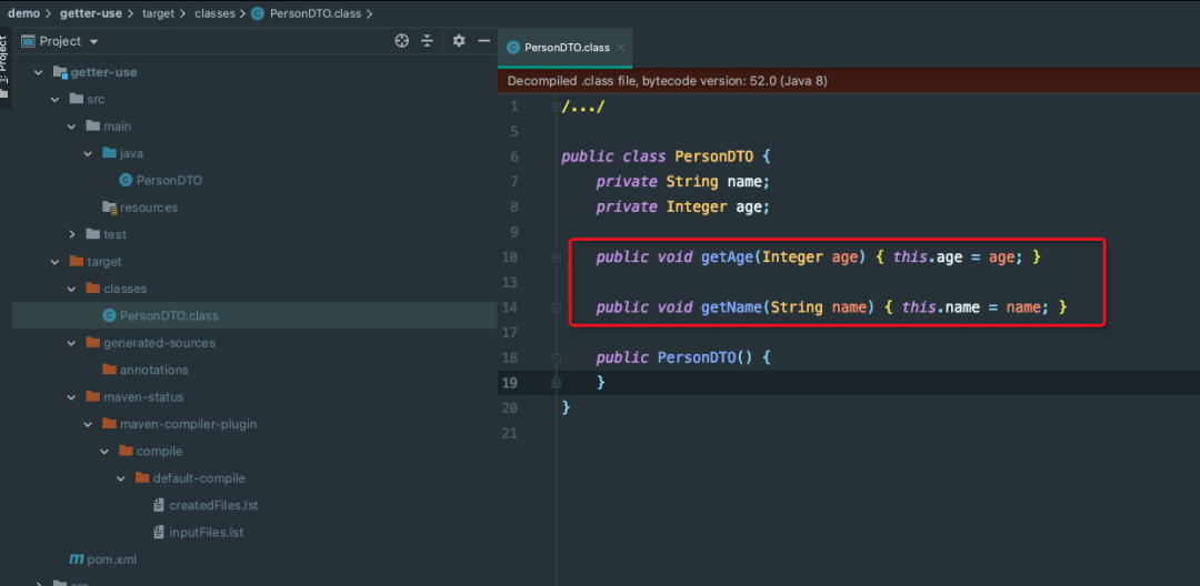
科普文:Lombok使用及工作原理详解
1. 概叙 Lombok是什么? Project Lombok 是一个 JAVA 库,它可以自动插入编辑器和构建工具,为您的 JAVA 锦上添花。再也不要写另一个 getter/setter 或 equals 等方法,只要有一个注注解,你的类就有一个功能齐全的生成器…...

飞致云开源社区月度动态报告(2024年7月)
自2023年6月起,中国领先的开源软件公司FIT2CLOUD飞致云以月度为单位发布《飞致云开源社区月度动态报告》,旨在向广大社区用户同步飞致云旗下系列开源软件的发展情况,以及当月主要的产品新版本发布、社区运营成果等相关信息。 飞致云开源大屏…...

mybatis-plus——实现动态字段排序,根据实体获取字段映射数据库的具体字段
前言 前端需要根据表头的点击控件可以排序,虽然前端能根据当前页的数据进行对应字段的排序,但也仅局限于实现当前页的排序,无法满足全部数据的排序,所以需要走接口的查询进行排序,获取最全的排序数据 实现方案 前端…...

redis:Linux安装redis,redis常用的数据类型及相关命令
1. 什么是NoSQL nosql[not only sql]不仅仅是sql。所有非关系型数据库的统称。除去关系型数据库之外的都是非关系数据库。 1.1为什么使用NoSQL NoSQL数据库相较于传统关系型数据库具有灵活性、可扩展性和高性能等优势,适合处理非结构化和半结构化数据,…...

JavaScript 和 HTML5 Canvas实现图像绘制与处理
前言 JavaScript 和 HTML5 的 canvas 元素提供了强大的图形和图像处理功能,使得开发者能够在网页上创建动态和交互式的视觉体验。这里我们将探讨如何使用 canvas 和 JavaScript 来处理图像加载,并在其上进行图像绘制。我们将实现一个简单的示例…...

Java之Java基础二十(集合[上])
Java 集合框架可以分为两条大的支线: ①、Collection,主要由 List、Set、Queue 组成: List 代表有序、可重复的集合,典型代表就是封装了动态数组的 ArrayList 和封装了链表的 LinkedList;Set 代表无序、不可重复的集…...

【C++BFS】1162. 地图分析
本文涉及知识点 CBFS算法 LeetCode1162. 地图分析 你现在手里有一份大小为 n x n 的 网格 grid,上面的每个 单元格 都用 0 和 1 标记好了。其中 0 代表海洋,1 代表陆地。 请你找出一个海洋单元格,这个海洋单元格到离它最近的陆地单元格的距…...
实战:安装ElasticSearch 和常用操作命令
概叙 科普文:深入理解ElasticSearch体系结构-CSDN博客 Elasticsearch各版本比较 ElasticSearch 单点安装 1 创建普通用户 #1 创建普通用户名,密码 [roothlink1 lyz]# useradd lyz [roothlink1 lyz]# passwd lyz#2 然后 关闭xshell 重新登录 ip 地址…...

React-Native 宝藏库大揭秘:精选开源项目与实战代码解析
1. 引言 1.1 React-Native 简介 React-Native 是由 Facebook 开发的一个开源框架,它允许开发者使用 JavaScript 和 React 的编程模型来构建跨平台的移动应用。React-Native 的核心理念是“Learn Once, Write Anywhere”,即学习一次 React 的编程模型&am…...

数据结构:二叉树(链式结构)
文章目录 1. 二叉树的链式结构2. 二叉树的创建和实现相关功能2.1 创建二叉树2.2 二叉树的前,中,后序遍历2.2.1 前序遍历2.2.2 中序遍历2.2.3 后序遍历 2.3 二叉树节点个数2.4 二叉树叶子结点个数2.5 二叉树第k层结点个数2.6 二叉树的深度/高度2.7 二叉树…...

召唤生命,阻止轻生——《生命门外》
本书的目的,就是阻止自杀!拉回那些深陷在这样的思维当中正在挣扎犹豫的人,提醒他们珍爱生命,让更多的人,尤其是年轻人从执迷不悟的犹豫徘徊中幡然醒悟,回归正常的生活。 网络上抱孩子跳桥轻生的母亲&#…...

JVM:栈上的数据存储
文章目录 一、Java虚拟机中的基本数据类型 一、Java虚拟机中的基本数据类型 在Java中有8大基本数据类型: 这里的内存占用,指的是堆上或者数组中内存分配的空间大小,栈上的实现更加复杂。 Java中的8大数据类型在虚拟机中的实现:…...

C#实战 - C#实现发送邮件的三种方法
作者:逍遥Sean 简介:一个主修Java的Web网站\游戏服务器后端开发者 主页:https://blog.csdn.net/Ureliable 觉得博主文章不错的话,可以三连支持一下~ 如有疑问和建议,请私信或评论留言! 前言 当使用 C# 编程…...

数模原理精解【5】
文章目录 二元分布满足要求边际分布条件概率例子1例子2 损失函数概率分布期望值例 参考文献 二元分布 满足要求 连续情况下, φ ( x , y ) \varphi (x,y) φ(x,y)为随机变量 X 、 Y X、Y X、Y的联合概率分布(二元分布),如果以下条件满足: …...
求解冷链路径优化问题的matlab代码(带说明文档))
基于遗传算法(GA)求解冷链路径优化问题的matlab代码(带说明文档)
✅作者简介:热爱科研的Matlab仿真开发者,擅长毕业设计辅导、数学建模、数据处理、建模仿真、程序设计、完整代码获取、论文复现及科研仿真。🍎 往期回顾关注个人主页:Matlab科研工作室👇 关注我领取海量matlab电子书和…...

5个HTTP请求配置技巧:让你的Dify工作流开发效率提升300%
5个HTTP请求配置技巧:让你的Dify工作流开发效率提升300% 【免费下载链接】Awesome-Dify-Workflow 分享一些好用的 Dify DSL 工作流程,自用、学习两相宜。 Sharing some Dify workflows. 项目地址: https://gitcode.com/GitHub_Trending/aw/Awesome-Dif…...

如何通过手机号快速找回QQ账号:3分钟完成的终极指南
如何通过手机号快速找回QQ账号:3分钟完成的终极指南 【免费下载链接】phone2qq 项目地址: https://gitcode.com/gh_mirrors/ph/phone2qq 还在为忘记QQ账号而烦恼吗?每次需要验证好友身份时都要翻遍通讯录?现在,通过phone2…...

Qwen3-0.6B-FP8实战:构建基于操作系统的命令行智能助手
Qwen3-0.6B-FP8实战:构建基于操作系统的命令行智能助手 你有没有过这样的经历?想用命令行完成一个任务,比如“找出所有昨天修改过的日志文件并压缩备份”,却记不清find命令那一长串复杂的参数,或者tar命令的语法又搞混…...

小样本学习:OpenClaw+nanobot镜像快速领域适配方案
小样本学习:OpenClawnanobot镜像快速领域适配方案 1. 为什么需要小样本领域适配 作为一名长期关注AI落地的开发者,我经常遇到这样的困境:通用大模型在垂直领域表现不佳,而从头训练专业模型又需要海量标注数据。直到发现OpenClaw…...

【已验证】基于STM32和HAL库的大夏龙雀BT311-10C02S蓝牙模块驱动
最近买了一个大夏龙雀家的蓝牙模块DX-BT311-10C02S,这个蓝牙是一款基于BLE 5.4规范的串口透传模块,支持AT指令配置、主从模式切换,非常适合与单片机搭配实现无线数据传输。如果是第一次买还是很便宜的,他家的模块有一说一是真的不…...
”)
【AI 智能体时代的软件工程】12 信任工程:建立 AI 时代的“三维材料清单 (BOM)”
大家好,我是Tony Bai。欢迎来到微专栏 《AI 智能体时代的软件工程》的第十二讲。在前面的课程中,我们从单体智能体的“任务简报(Mission Brief)”,一路讲到了多智能体协同的“自动化流水线”,并在上一讲为你…...

终极GPU显存检测指南:使用memtest_vulkan轻松诊断显卡稳定性问题
终极GPU显存检测指南:使用memtest_vulkan轻松诊断显卡稳定性问题 【免费下载链接】memtest_vulkan Vulkan compute tool for testing video memory stability 项目地址: https://gitcode.com/gh_mirrors/me/memtest_vulkan 显卡显存稳定性直接影响着游戏体验…...
)
从动漫生成到金融风控:LSGAN损失函数在5个行业的落地对比(附数据集下载)
从动漫生成到金融风控:LSGAN损失函数在5个行业的落地对比 当生成对抗网络(GAN)遇上最小二乘损失函数(LSGAN),会擦出怎样的火花?这个看似简单的数学改进,正在悄然改变多个行业的AI应用…...

HunyuanVideo-Foley 安全与权限管理:企业内网API访问控制实践
HunyuanVideo-Foley 安全与权限管理:企业内网API访问控制实践 1. 企业AI服务的安全挑战 随着AI技术在企业内部的广泛应用,视频处理类API的安全管理成为IT部门的新课题。HunyuanVideo-Foley作为专业的音视频处理工具,在私有化部署场景下需要…...