Python精选200Tips:186-190
针对序列(时间、文本)数据的网络结构 续
- P186-- 双向LSTM(Bidirectional Long Short-Term Memory 2005)
- (1)模型结构说明
- (2)创新性说明
- (3)示例代码:IMDB电影评论情感分析
- P187--变换器结构(Transformer 2017)
- (1)模型结构说明
- (2)创新性说明
- (3)示例代码:模拟气象数据预测(多输出多输出)
- P188-- 时间卷积网络(TCN,Temporal Convolutional Network 2018)
- (1)模型结构说明
- (2)创新性说明
- (3)示例代码:模拟气象数据预测(多输出多输出)
- P189-- CNN+LSTM混合模型
- (1)模型结构说明
- (2)创新性说明
- (3)示例代码:模拟气象数据预测(多输出多输出)
- P190-- Informer结构 2020
- (1)模型结构说明
- (2)创新性说明
- (3)示例代码:模拟气象数据预测(多输出多输出)
运行系统:macOS Sequoia 15.0
Python编译器:PyCharm 2024.1.4 (Community Edition)
Python版本:3.12
TensorFlow版本:2.17.0
Pytorch版本:2.4.1
往期链接:
| 1-5 | 6-10 | 11-20 | 21-30 | 31-40 | 41-50 |
|---|
| 51-60:函数 | 61-70:类 | 71-80:编程范式及设计模式 |
|---|
| 81-90:Python编码规范 | 91-100:Python自带常用模块-1 |
|---|
| 101-105:Python自带模块-2 | 106-110:Python自带模块-3 |
|---|
| 111-115:Python常用第三方包-频繁使用 | 116-120:Python常用第三方包-深度学习 |
|---|
| 121-125:Python常用第三方包-爬取数据 | 126-130:Python常用第三方包-为了乐趣 |
|---|
| 131-135:Python常用第三方包-拓展工具1 | 136-140:Python常用第三方包-拓展工具2 |
|---|
Python项目实战
| 141-145 | 146-150 | 151-155 | 156-160 | 161-165 | 166-170 | 171-175 |
|---|
| 176-180:卷积结构 | 181-182:卷积结构(续) | 183-185:时间、序列数据 |
|---|
P186-- 双向LSTM(Bidirectional Long Short-Term Memory 2005)
(1)模型结构说明
2005年,Alex Graves和Jürgen Schmidhuber将双向RNN的概念应用于LSTM,正式提出了双向LSTM架构。这一创新使得LSTM能够同时利用序列的过去和未来上下文信息,从而提升了在许多序列建模任务中的表现。双向LSTM(Bidirectional Long Short-Term Memory)是对传统LSTM的一种扩展,旨在同时考虑序列的过去和未来信息。其工作原理包括:
结构:由两个独立的LSTM层组成,一个按正向(从左到右)处理输入序列,另一个按反向(从右到左)处理同一序列。
信息流:每个时间步的输出结合了来自两个方向的信息,这样模型能更好地捕捉上下文。
输出:两个LSTM的输出通常被连接或合并,以供后续处理。
(2)创新性说明
双向信息流
正向与反向处理:双向LSTM通过两个独立的LSTM层,一个从序列的开始到结束(正向),另一个从结束到开始(反向)处理信息。这种双向处理方式使得模型能够同时利用过去和未来的上下文信息。
上下文理解
全面的上下文捕捉:传统LSTM只能利用过去的信息,而双向LSTM能够捕捉到完整的上下文信息。这对许多自然语言处理任务(如命名实体识别、情感分析等)至关重要,因为这些任务常常需要理解语句的前后关系。
更丰富的特征表示
融合信息:双向LSTM结合了正向和反向的输出,提供了更丰富的特征表示。这种综合特征增强了模型对复杂模式的捕捉能力,有助于提高预测的准确性。
改进的性能
在多种任务中的表现:双向LSTM在许多序列建模任务中表现优于单向LSTM,特别是在需要理解完整上下文的场景,如文本分类、机器翻译等。
适应性强
广泛应用:双向LSTM适用于多种序列数据的任务,不仅限于文本,还可以应用于语音识别、时间序列预测等领域,显示了其广泛的适应性。
解决长距离依赖问题
缓解梯度消失:通过结合双向信息流,双向LSTM在一定程度上缓解了长距离依赖问题,使得模型能够更好地学习长期依赖关系。
(3)示例代码:IMDB电影评论情感分析
import tensorflow as tf
from tensorflow.keras.datasets import imdb
from tensorflow.keras.preprocessing.sequence import pad_sequences
from tensorflow.keras.models import Sequential
from tensorflow.keras.layers import Embedding, Bidirectional, LSTM, Dense# 设置参数
max_features = 20000
maxlen = 100
batch_size = 32
embedding_dims = 128
epochs = 5# 加载IMDB数据集
(x_train, y_train), (x_test, y_test) = imdb.load_data(num_words=max_features)# 填充序列
x_train = pad_sequences(x_train, maxlen=maxlen)
x_test = pad_sequences(x_test, maxlen=maxlen)# 构建模型
model = Sequential()
model.add(Embedding(max_features, embedding_dims, input_length=maxlen))
model.add(Bidirectional(LSTM(64)))
model.add(Dense(1, activation='sigmoid'))# 编译模型
model.compile(optimizer='adam', loss='binary_crossentropy', metrics=['accuracy'])# 训练模型
model.fit(x_train, y_train, batch_size=batch_size, epochs=epochs, validation_split=0.2)# 评估模型
score, acc = model.evaluate(x_test, y_test, batch_size=batch_size)
print(f'Test score: {score}, Test accuracy: {acc}')# 预测情感
def predict_sentiment(review):sequence = imdb.get_word_index()sequence = [sequence.get(word, 0) for word in review.lower().split()]sequence = pad_sequences([sequence], maxlen=maxlen)prediction = model.predict(sequence)return "Positive" if prediction[0][0] > 0.5 else "Negative"# 测试预测
sample_review = "This movie was fantastic!"
print(f"Sample review: {sample_review}")
print(f"Predicted sentiment: {predict_sentiment(sample_review)}")

P187–变换器结构(Transformer 2017)
(1)模型结构说明
Transformer模型是由Vaswani等人在2017年的论文"Attention Is All You Need"中提出的。这个模型在自然语言处理领域产生了革命性的影响,并且后来被扩展到其他领域如计算机视觉。Transformer的核心原理是完全基于注意力机制(Attention Mechanism)的序列到序列(Sequence-to-Sequence)模型。原理如下:
自注意力机制(Self-Attention):允许模型在处理序列中的每个位置时,都能关注到序列中的其他所有位置。
多头注意力(Multi-Head Attention):允许模型同时关注不同的表示子空间。
位置编码(Positional Encoding):由于模型不含递归或卷积,使用位置编码来为模型提供序列中的位置信息。
编码器-解码器结构 :模型包含多层编码器和解码器,每层都包含自注意力机制和前馈神经网络。
(2)创新性说明
全注意力架构:首次提出完全基于注意力机制的模型,摒弃了之前广泛使用的RNN和CNN结构。
多头注意力:创新性地提出了多头注意力机制,增强了模型的表达能力。
位置编码:巧妙地解决了序列顺序信息的问题,而不需要引入递归结构。
残差连接和层归一化:在每个子层后使用残差连接和层归一化,有助于训练更深的网络。
缩放点积注意力:通过缩放因子改进了注意力计算的稳定性。
并行训练:设计了可以高度并行化的结构,大大提高了训练效率。
Transformer模型的创新性在于它完全重新思考了序列处理的方式。它证明了仅仅依靠注意力机制就能达到甚至超越之前最先进的基于RNN的模型的性能。
(3)示例代码:模拟气象数据预测(多输出多输出)
import numpy as np
import tensorflow as tf
from tensorflow import keras
from tensorflow.keras import layers
import matplotlib.pyplot as plt# 1. 数据生成
def generate_weather_data(n_samples, n_steps):time = np.linspace(0, 1, n_steps)# 温度:基础温度 + 季节变化 + 日间变化 + 随机噪声temp_seasonal = 10 * np.sin(2 * np.pi * time)  # 季节变化temp_daily = 5 * np.sin(2 * np.pi * time * n_steps)  # 日间变化temp = 15 + temp_seasonal + temp_daily + np.random.normal(0, 2, (n_samples, n_steps))# 湿度:与温度负相关 + 随机噪声humidity = 100 - temp / 40 * 100 + np.random.normal(0, 5, (n_samples, n_steps))humidity = np.clip(humidity, 0, 100)# 风速:使用 Gamma 分布随机生成wind_speed = np.random.gamma(2, 2, (n_samples, n_steps))# 合并数据data = np.stack([temp, humidity, wind_speed], axis=-1)  # 形状:(n_samples, n_steps, 3)return data.astype(np.float32)# 2. 数据准备
n_samples = 10000
n_steps = 100  # 输入时间步数
n_future = 24  # 预测未来的时间步数
data = generate_weather_data(n_samples, n_steps + n_future)X = data[:, :n_steps, :]  # 输入特征:温度、湿度、风速
y = data[:, n_steps:, :2]  # 输出目标:未来的温度和湿度# 划分训练集、验证集和测试集
train_size = int(n_samples * 0.7)
val_size = int(n_samples * 0.9)X_train = X[:train_size]
y_train = y[:train_size]X_val = X[train_size:val_size]
y_val = y[train_size:val_size]X_test = X[val_size:]
y_test = y[val_size:]n_features = X_train.shape[2]  # 输入特征数:3(温度、湿度、风速)# 3. 定义 Positional Encoding
class PositionalEncoding(layers.Layer):def __init__(self, sequence_length, embed_dim):super(PositionalEncoding, self).__init__()self.pos_encoding = self.positional_encoding(sequence_length, embed_dim)def get_angles(self, pos, i, embed_dim):angles = pos / np.power(10000, (2 * (i // 2)) / np.float32(embed_dim))return anglesdef positional_encoding(self, sequence_length, embed_dim):angle_rads = self.get_angles(np.arange(sequence_length)[:, np.newaxis],np.arange(embed_dim)[np.newaxis, :],embed_dim)# 将 sin 应用于偶数索引(2i)sines = np.sin(angle_rads[:, 0::2])# 将 cos 应用于奇数索引(2i+1)cosines = np.cos(angle_rads[:, 1::2])pos_encoding = np.zeros((sequence_length, embed_dim))pos_encoding[:, 0::2] = sinespos_encoding[:, 1::2] = cosinespos_encoding = pos_encoding[np.newaxis, ...]return tf.cast(pos_encoding, dtype=tf.float32)def call(self, inputs):return inputs + self.pos_encoding# 4. 定义 TransformerBlock
class TransformerBlock(layers.Layer):def __init__(self, embed_dim, num_heads, ff_dim, rate=0.1):super(TransformerBlock, self).__init__()self.att = layers.MultiHeadAttention(num_heads=num_heads, key_dim=embed_dim)self.ffn = keras.Sequential([layers.Dense(ff_dim, activation='relu'),layers.Dense(embed_dim)])self.layernorm1 = layers.LayerNormalization(epsilon=1e-6)self.layernorm2 = layers.LayerNormalization(epsilon=1e-6)self.dropout1 = layers.Dropout(rate)self.dropout2 = layers.Dropout(rate)def call(self, inputs, training=None):attn_output = self.att(inputs, inputs, training=training)attn_output = self.dropout1(attn_output, training=training)out1 = self.layernorm1(inputs + attn_output)ffn_output = self.ffn(out1)ffn_output = self.dropout2(ffn_output, training=training)return self.layernorm2(out1 + ffn_output)# 5. 构建 Transformer 模型
def build_transformer_model(input_shape, embed_dim, num_heads, ff_dim, num_layers, dropout, n_future,n_output_features):inputs = keras.Input(shape=input_shape)  # 输入形状:(n_steps, n_features)# 投影到嵌入维度x = layers.Dense(embed_dim)(inputs)# 添加位置编码x = PositionalEncoding(input_shape[0], embed_dim)(x)# 堆叠 Transformer 块for _ in range(num_layers):x = TransformerBlock(embed_dim, num_heads, ff_dim, rate=dropout)(x)# 全局平均池化x = layers.GlobalAveragePooling1D()(x)# 全连接层x = layers.Dense(64, activation='relu')(x)x = layers.Dropout(dropout)(x)x = layers.Dense(n_future * n_output_features)(x)outputs = layers.Reshape((n_future, n_output_features))(x)model = keras.Model(inputs=inputs, outputs=outputs)return model# 6. 设置模型参数并构建模型
input_shape = (n_steps, n_features)
embed_dim = 64
num_heads = 4
ff_dim = 128
num_layers = 2
dropout = 0.1
n_output_features = y_train.shape[2]  # 输出特征数:2(温度和湿度)model = build_transformer_model(input_shape, embed_dim, num_heads, ff_dim, num_layers, dropout, n_future, n_output_features
)# 7. 编译和训练模型
model.compile(optimizer='adam', loss='mse', metrics=['mae'])history = model.fit(X_train, y_train,validation_data=(X_val, y_val),epochs=20,batch_size=64
)# 8. 评估模型
loss, mae = model.evaluate(X_test, y_test)
print(f'Test MAE: {mae}')# 9. 可视化训练过程
plt.figure(figsize=(10, 6))
plt.plot(history.history['loss'], label='Train Loss')
plt.plot(history.history['val_loss'], label='Validation Loss')
plt.xlabel('Epoch')
plt.ylabel('MSE Loss')
plt.legend()
plt.title('Training and Validation Loss')
plt.show()# 10. 进行预测并可视化结果
# 生成新数据进行预测
X_new = generate_weather_data(1, n_steps)
y_pred = model.predict(X_new)# 绘制预测结果
plt.figure(figsize=(12, 8))# 温度预测
plt.subplot(2, 1, 1)
plt.plot(range(n_steps), X_new[0, :, 0], label='Historical Temperature')
plt.plot(range(n_steps, n_steps + n_future), y_pred[0, :, 0], label='Predicted Temperature')
plt.xlabel('Time Step')
plt.ylabel('Temperature')
plt.legend()
plt.title('Temperature Prediction')# 湿度预测
plt.subplot(2, 1, 2)
plt.plot(range(n_steps), X_new[0, :, 1], label='Historical Humidity')
plt.plot(range(n_steps, n_steps + n_future), y_pred[0, :, 1], label='Predicted Humidity')
plt.xlabel('Time Step')
plt.ylabel('Humidity')
plt.legend()
plt.title('Humidity Prediction')plt.tight_layout()
plt.show()
P188-- 时间卷积网络(TCN,Temporal Convolutional Network 2018)
(1)模型结构说明
Bai、Kolter和Koltun发表了题为"An Empirical Evaluation of Generic Convolutional and Recurrent Networks for Sequence Modeling"的论文。这篇论文正式提出了本节介绍的TCN架构。时间卷积网络(Temporal Convolutional Network,TCN)是一种专门用于处理时间序列数据的深度学习模型。下面我将详细介绍其原理、特点和实际应用例子。
原理
因果卷积:TCN使用因果卷积,确保t时刻的输出只依赖于t时刻及之前的输入,避免信息泄露。
膨胀卷积:通过在卷积核中引入间隔,增大感受野,捕捉长期依赖关系。
残差连接:使用残差块,有助于训练更深的网络并缓解梯度消失问题。
层级结构:通过堆叠多层卷积,逐步提取更高层次的时间特征。
(2)创新性说明
并行处理:相比RNN,TCN可以并行处理输入序列,提高计算效率。
固定感受野:每层的膨胀卷积可以精确控制网络的感受野大小。
灵活的序列长度:可以处理任意长度的输入序列。
稳定梯度:避免了RNN中的梯度消失/爆炸问题。
内存效率:相比LSTM,TCN的内存占用随序列长度的增加而增加得较慢。
(3)示例代码:模拟气象数据预测(多输出多输出)
import numpy as np
import tensorflow as tf
from tensorflow.keras.layers import Input, Conv1D, Dense, Dropout, LayerNormalization, Activation, \GlobalAveragePooling1D
from tensorflow.keras.models import Model# TCN残差块
def residual_block(x, dilation_rate, nb_filters, kernel_size):padding = (kernel_size - 1) * dilation_rater = Conv1D(filters=nb_filters, kernel_size=kernel_size,dilation_rate=dilation_rate, padding='causal')(x)r = LayerNormalization()(r)r = Activation('relu')(r)r = Dropout(0.1)(r)r = Conv1D(filters=nb_filters, kernel_size=kernel_size,dilation_rate=dilation_rate, padding='causal')(r)r = LayerNormalization()(r)r = Activation('relu')(r)r = Dropout(0.1)(r)if x.shape[-1] != nb_filters:x = Conv1D(filters=nb_filters, kernel_size=1, padding='same')(x)return tf.keras.layers.add([x, r])# TCN模型
def build_tcn_model(input_shape, nb_filters, kernel_size, nb_stacks, dilations, output_dim):input_layer = Input(shape=input_shape)x = input_layerfor _ in range(nb_stacks):for d in dilations:x = residual_block(x, d, nb_filters, kernel_size)# 使用GlobalAveragePooling1D来将时间维度压缩x = GlobalAveragePooling1D()(x)x = Dense(64, activation='relu')(x)output = Dense(output_dim)(x)model = Model(inputs=input_layer, outputs=output)return model# 生成示例数据
def generate_data(n_samples, n_timesteps, n_features_in, n_features_out):X = np.random.randn(n_samples, n_timesteps, n_features_in)y = np.random.randn(n_samples, n_features_out)return X, y# 设置参数
n_samples = 1000
n_timesteps = 10
n_features_in = 3  # 温度、湿度、风速
n_features_out = 2  # 预测未来的温度和湿度# 生成数据
X, y = generate_data(n_samples, n_timesteps, n_features_in, n_features_out)# 构建模型
input_shape = (n_timesteps, n_features_in)
model = build_tcn_model(input_shape, nb_filters=64, kernel_size=3, nb_stacks=1,dilations=[1, 2, 4, 8], output_dim=n_features_out)# 编译模型
model.compile(optimizer='adam', loss='mse')# 打印模型摘要
model.summary()# 训练模型
history = model.fit(X, y, epochs=50, batch_size=32, validation_split=0.2, verbose=1)# 生成测试数据
X_test, y_test = generate_data(10, n_timesteps, n_features_in, n_features_out)# 预测
predictions = model.predict(X_test)# 打印预测结果
for i in range(10):print(f"Sample {i + 1}:")print(f"Predicted Temperature: {predictions[i][0]:.2f}, Actual: {y_test[i][0]:.2f}")print(f"Predicted Humidity: {predictions[i][1]:.2f}, Actual: {y_test[i][1]:.2f}")print()
P189-- CNN+LSTM混合模型
(1)模型结构说明
原理
CNN部分:
CNN通过卷积层提取输入数据中的局部特征,适用于处理图像、时序数据等。
主要用于捕捉空间特征,如气象数据中的空间相关性。
LSTM部分:
LSTM通过其特殊的门控机制(输入门、遗忘门、输出门)来控制信息的流动,能够记忆长时间的依赖关系。
适合处理时间序列数据,保留过去信息以进行未来预测。
结合机制:
CNN首先对输入数据进行特征提取,然后将提取的特征输入到LSTM中进行时间序列建模。
通过这种方式,CNN负责捕捉数据中的空间模式,LSTM则负责处理时间序列的动态变化。
(2)创新性说明
多模态特征提取:通过结合CNN的空间特征提取能力和LSTM的时间建模能力,使得模型能够处理复杂的时空数据。
提高预测精度:在气象预测等任务中,CNN+LSTM的组合能够显著提高预测精度,尤其是在需要考虑长期依赖关系的情况下。
应用广泛:这种结合的模型在视频分析、语音识别、气象预测等多个领域表现出色,成为深度学习中的一种重要架构。
(3)示例代码:模拟气象数据预测(多输出多输出)
import numpy as np
import torch
import torch.nn as nn
import torch.optim as optim
import matplotlib.pyplot as plt# macos系统显示中文
plt.rcParams['font.sans-serif'] = ['Arial Unicode MS']# 生成模拟的气象数据
def generate_weather_data(samples=1000, timesteps=24, features=3):data = np.zeros((samples, timesteps, features))for i in range(samples):base_temp = 15 + np.random.rand() * 10      # 基础温度在 15 到 25 度之间base_humidity = 50 + np.random.rand() * 50  # 基础湿度在 50% 到 100% 之间base_pressure = 1000 + np.random.rand() * 50 # 基础气压在 1000 到 1050 hPa 之间for t in range(timesteps):data[i, t, 0] = base_temp + np.sin(t / timesteps * 2 * np.pi) * 10 + np.random.randn()  # 温度随时间变化data[i, t, 1] = base_humidity + np.cos(t / timesteps * 2 * np.pi) * 20 + np.random.randn()  # 湿度随时间变化data[i, t, 2] = base_pressure + np.sin(t / timesteps * 4 * np.pi) * 5 + np.random.randn()  # 气压随时间变化return data# 创建数据集
def create_dataset(data, seq_length, pred_length):X, y = [], []for sample in data:for i in range(len(sample) - seq_length - pred_length + 1):X.append(sample[i:i + seq_length])y.append(sample[i + seq_length:i + seq_length + pred_length])return np.array(X), np.array(y)# 准备数据
# 设置参数
samples = 1000
timesteps = 24
features = 3      # 温度、湿度、气压
seq_length = 12   # 输入序列长度
pred_length = 6   # 预测序列长度# 生成数据
data = generate_weather_data(samples, timesteps, features)# 创建数据集
X, y = create_dataset(data, seq_length, pred_length)# 划分训练集和测试集
train_size = int(len(X) * 0.8)
X_train = X[:train_size]
y_train = y[:train_size]
X_test = X[train_size:]
y_test = y[train_size:]# 转换为 PyTorch 张量
X_train_tensor = torch.tensor(X_train, dtype=torch.float32)
y_train_tensor = torch.tensor(y_train, dtype=torch.float32)
X_test_tensor = torch.tensor(X_test, dtype=torch.float32)
y_test_tensor = torch.tensor(y_test, dtype=torch.float32)# 定义 CNN+LSTM 模型
class CNNLSTM(nn.Module):def __init__(self, input_size, hidden_size, num_layers, seq_length, pred_length, num_features):super(CNNLSTM, self).__init__()self.num_features = num_featuresself.pred_length = pred_length# 定义卷积层self.conv1 = nn.Conv1d(in_channels=num_features, out_channels=64, kernel_size=3, padding=1)self.relu1 = nn.ReLU()self.pool1 = nn.MaxPool1d(kernel_size=2)# 计算卷积和池化后的序列长度conv_seq_length = seq_length // 2  # 池化层会将序列长度减半# 定义 LSTM 层self.lstm = nn.LSTM(input_size=64, hidden_size=hidden_size, num_layers=num_layers, batch_first=True)# 定义全连接层self.fc = nn.Linear(hidden_size, num_features * pred_length)def forward(self, x):# x: (batch_size, seq_length, num_features)x = x.permute(0, 2, 1)  # 转换为 (batch_size, num_features, seq_length)x = self.conv1(x)x = self.relu1(x)x = self.pool1(x)       # (batch_size, out_channels, seq_length // 2)x = x.permute(0, 2, 1)  # 转换为 (batch_size, seq_length // 2, out_channels)# LSTM 层x, _ = self.lstm(x)     # x: (batch_size, seq_length // 2, hidden_size)x = x[:, -1, :]         # 取最后一个时间步的输出 (batch_size, hidden_size)# 全连接层x = self.fc(x)          # (batch_size, num_features * pred_length)x = x.view(-1, self.pred_length, self.num_features)  # (batch_size, pred_length, num_features)return x# 实例化模型并定义损失函数与优化器
input_size = features
hidden_size = 128
num_layers = 2model = CNNLSTM(input_size=input_size, hidden_size=hidden_size, num_layers=num_layers, seq_length=seq_length, pred_length=pred_length, num_features=features)criterion = nn.MSELoss()
optimizer = optim.Adam(model.parameters(), lr=0.001)# 训练模型
# 训练参数
epochs = 20
batch_size = 64# 创建数据加载器
train_dataset = torch.utils.data.TensorDataset(X_train_tensor, y_train_tensor)
train_loader = torch.utils.data.DataLoader(train_dataset, batch_size=batch_size, shuffle=True)# 训练循环
for epoch in range(epochs):model.train()total_loss = 0for X_batch, y_batch in train_loader:optimizer.zero_grad()outputs = model(X_batch)loss = criterion(outputs, y_batch)loss.backward()optimizer.step()total_loss += loss.item()avg_loss = total_loss / len(train_loader)print(f'Epoch [{epoch+1}/{epochs}], Loss: {avg_loss:.4f}')# 测试模型
model.eval()
with torch.no_grad():test_outputs = model(X_test_tensor)test_loss = criterion(test_outputs, y_test_tensor)print(f'Test Loss: {test_loss.item():.4f}')# 选择一个样本进行可视化
index = 0
input_sample = X_test_tensor[index].numpy()
target_sample = y_test_tensor[index].numpy()
prediction = test_outputs[index].numpy()# 绘制结果
time_input = np.arange(seq_length)
time_pred = np.arange(seq_length, seq_length + pred_length)plt.figure(figsize=(12, 8))
feature_names = ['温度', '湿度', '气压']
for i in range(features):plt.subplot(features, 1, i+1)plt.plot(time_input, input_sample[:, i], label='历史数据')plt.plot(time_pred, target_sample[:, i], label='真实值')plt.plot(time_pred, prediction[:, i], label='预测值', linestyle='--')plt.title(f'特征 {feature_names[i]} 的预测')plt.xlabel('时间步')plt.ylabel(f'{feature_names[i]}')plt.legend()
plt.tight_layout()
plt.show()

P190-- Informer结构 2020
(1)模型结构说明
Informer由清华大学和华为诺亚方舟实验室的研究团队在2020年提出,旨在解决传统Transformer在处理长序列时的计算效率问题。该模型在AAAI 2021会议上发表,成为时序预测领域的重要进展。详细原理如下:
架构基础
Informer基于标准Transformer架构,但针对长序列进行了优化。
ProbSparse自注意力机制
通过引入ProbSparse机制,Informer在计算自注意力时只关注最重要的部分。这种策略显著降低了计算复杂度。
自注意力蒸馏
在模型的不同层中逐渐减少序列长度,使得后续层的计算更加高效。
生成式解码器
Informer使用生成式解码器,一次性预测长序列,避免了自回归模型的累积误差。
数据嵌入
使用专门的数据嵌入层处理不同特征(如时间特征),增强模型对时序数据的理解能力。
(2)创新性说明
效率提升:通过ProbSparse自注意力机制,Informer能够在保持高精度的同时,显著减少计算资源的消耗。
长序列处理:优化后的自注意力机制使得模型能够有效处理长序列数据,克服了传统Transformer的局限性。
灵活性:生成式解码器的引入使得模型在处理复杂预测任务时表现更加出色。
(3)示例代码:模拟气象数据预测(多输出多输出)
# 导入必要的库
import numpy as np
import torch
import torch.nn as nn
import torch.optim as optim
import matplotlib.pyplot as plt# macos系统显示中文
plt.rcParams['font.sans-serif'] = ['Arial Unicode MS']# 1. 生成模拟的气象数据
def generate_weather_data(num_samples=1000, seq_len=100, num_features=3):# 生成随机数据data = np.random.randn(num_samples, seq_len, num_features)# 添加趋势和季节性因素for i in range(num_features):trend = np.linspace(0, 1, seq_len)seasonality = np.sin(np.linspace(0, 2 * np.pi, seq_len))data[:, :, i] += trend + seasonality + np.random.randn(num_samples, seq_len) * 0.1return data# 2. 准备数据集
def create_dataset(data, input_length, output_length):X, y = [], []num_samples, seq_len, num_features = data.shapefor i in range(num_samples):if seq_len < input_length + output_length:continuefor j in range(seq_len - input_length - output_length + 1):X.append(data[i, j:j + input_length, :])y.append(data[i, j + input_length:j + input_length + output_length, :])return np.array(X), np.array(y)# 3. 生成数据
num_samples = 1000
seq_len = 100
num_features = 3  # 例如,温度、湿度、风速
data = generate_weather_data(num_samples, seq_len, num_features)input_length = 60  # 输入序列长度
output_length = 10  # 预测序列长度# 4. 创建数据集
X, y = create_dataset(data, input_length, output_length)
print("Input shape:", X.shape)  # (样本数, 输入长度, 特征数)
print("Output shape:", y.shape)  # (样本数, 输出长度, 特征数)# 5. 划分训练集和测试集
from sklearn.model_selection import train_test_splitX_train, X_test, y_train, y_test = train_test_split(X, y, test_size=0.2, random_state=42
)# 转换为 PyTorch 的张量
X_train_tensor = torch.tensor(X_train, dtype=torch.float32)
y_train_tensor = torch.tensor(y_train, dtype=torch.float32)
X_test_tensor = torch.tensor(X_test, dtype=torch.float32)
y_test_tensor = torch.tensor(y_test, dtype=torch.float32)# 6. 定义简化的 Informer 模型
class Informer(nn.Module):def __init__(self, input_dim, d_model, n_heads, e_layers, d_ff, dropout, output_dim, seq_len, pred_len):super(Informer, self).__init__()self.seq_len = seq_lenself.pred_len = pred_len# 输入嵌入层self.enc_embedding = nn.Linear(input_dim, d_model)# 位置编码(可选,简单起见使用参数)self.positional_encoding = nn.Parameter(torch.zeros(1, seq_len, d_model))# Transformer 编码器层encoder_layer = nn.TransformerEncoderLayer(d_model=d_model, nhead=n_heads, dim_feedforward=d_ff, dropout=dropout)self.encoder = nn.TransformerEncoder(encoder_layer, num_layers=e_layers)# 全连接输出层self.projection = nn.Linear(d_model, output_dim)def forward(self, x_enc):"""x_enc: (batch_size, seq_len, input_dim)"""# 输入嵌入x = self.enc_embedding(x_enc)  # (batch_size, seq_len, d_model)x += self.positional_encoding  # 添加位置编码x = x.permute(1, 0, 2)  # (seq_len, batch_size, d_model)# Transformer 编码器enc_output = self.encoder(x)  # (seq_len, batch_size, d_model)enc_output = enc_output[-self.pred_len:, :, :]  # 取最后 pred_len 个时间步enc_output = enc_output.permute(1, 0, 2)  # (batch_size, pred_len, d_model)# 全连接输出output = self.projection(enc_output)  # (batch_size, pred_len, output_dim)return output# 7. 实例化模型并定义损失函数和优化器
input_dim = num_features
output_dim = num_features
d_model = 64
n_heads = 4
e_layers = 2
d_ff = 128
dropout = 0.1
seq_len = input_length
pred_len = output_lengthmodel = Informer(input_dim, d_model, n_heads, e_layers, d_ff, dropout,output_dim, seq_len, pred_len
)# 定义损失函数和优化器
criterion = nn.MSELoss()
optimizer = optim.Adam(model.parameters(), lr=0.001)# 8. 训练模型
import timeepochs = 10
batch_size = 64train_dataset = torch.utils.data.TensorDataset(X_train_tensor, y_train_tensor)
train_loader = torch.utils.data.DataLoader(train_dataset, batch_size=batch_size, shuffle=True
)for epoch in range(epochs):start_time = time.time()model.train()total_loss = 0for batch_x, batch_y in train_loader:optimizer.zero_grad()output = model(batch_x)loss = criterion(output, batch_y)loss.backward()optimizer.step()total_loss += loss.item()avg_loss = total_loss / len(train_loader)elapsed = time.time() - start_timeprint(f'Epoch {epoch + 1}/{epochs}, Loss: {avg_loss:.4f}, Time: {elapsed:.2f}s')# 9. 测试模型并可视化结果
model.eval()
with torch.no_grad():test_output = model(X_test_tensor)test_loss = criterion(test_output, y_test_tensor)print(f'Test Loss: {test_loss.item():.4f}')# 可视化预测结果(以第一个测试样本为例)
sample_input = X_test_tensor[0].unsqueeze(0)  # (1, input_length, num_features)
sample_output = y_test_tensor[0].unsqueeze(0)  # (1, output_length, num_features)
with torch.no_grad():sample_pred = model(sample_input)  # (1, output_length, num_features)sample_input = sample_input.numpy().squeeze()
sample_output = sample_output.numpy().squeeze()
sample_pred = sample_pred.numpy().squeeze()time_input = np.arange(input_length)
time_output = np.arange(input_length, input_length + output_length)plt.figure(figsize=(12, 8))
for i in range(num_features):plt.subplot(num_features, 1, i + 1)plt.plot(time_input, sample_input[:, i], label=f'输入特征 {i + 1}')plt.plot(time_output, sample_output[:, i], label=f'真实未来特征 {i + 1}')plt.plot(time_output, sample_pred[:, i], label=f'预测未来特征 {i + 1}')plt.legend()plt.xlabel('时间步')plt.ylabel('特征值')plt.title(f'特征 {i + 1} 的预测结果')
plt.tight_layout()
plt.show()

相关文章:
Python精选200Tips:186-190
针对序列(时间、文本)数据的网络结构 续 P186-- 双向LSTM(Bidirectional Long Short-Term Memory 2005)(1)模型结构说明(2)创新性说明(3)示例代码:IMDB电影评论情感分析 …...

C、C++常用数据结构:链表
文章目录 基本概念链表的创建链表结点定义链表创建 链表遍历链表释放链表查找链表删除链表插入测试用例 基本概念 参考:链表基础知识详解(非常详细简单易懂)-CSDN博客 链表是一种线性存储结构,链表在物理存储上是非连续的…...

【devops】devops-ansible之剧本变量使用
本站以分享各种运维经验和运维所需要的技能为主 《python零基础入门》:python零基础入门学习 《python运维脚本》: python运维脚本实践 《shell》:shell学习 《terraform》持续更新中:terraform_Aws学习零基础入门到最佳实战 《k8》从问题中去学习k8s 《docker学习》暂未更…...

《Linux从小白到高手》理论篇:一文概览常用Linux重要配置文件
List item 今天继续宅家,闲来无事接着写。本篇是《Linux从小白到高手》理论篇的最后一篇了。本篇集中介绍所有常用的Linux重要配置文件。 用这个命令可以查看配置文件所在的位置:如上图 locate "*.conf" "*.ini" "*.cfg&quo…...

采购管理流程:掌握最后阶段的关键要点
采购管理流程是企业运作中的核心职能之一,涵盖了获取商品和服务的一系列步骤,旨在以高效率和经济效益的方式进行。深入理解该流程的每个环节极为关键,特别是最后阶段,这可确保所有采购活动的圆满完成以及与供应商维持良好关系。 …...
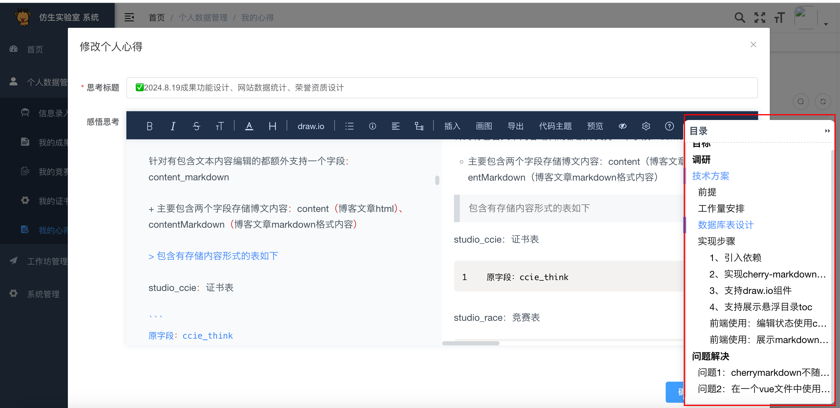
cherry-markdown开源markdown组件详细使用教程
文章目录 前言开发定位目标调研技术方案前提工作量安排数据库表设计实现步骤1、引入依赖2、实现cherry-markdown的vue组件(修改上传接口路径)3、支持draw.io组件4、支持展示悬浮目录toc前端使用:编辑状态使用cherry-markdown的vue组件前端使用…...

Android SystemUI组件(10)禁用/重启锁屏流程分析
该系列文章总纲链接:专题分纲目录 Android SystemUI组件 本章关键点总结 & 说明: 说明:本章节持续迭代之前章节的思维导图,主要关注左侧上方锁屏分析部分 应用入口处理流程解读 即可。 在 Android 系统中,禁用锁屏…...

【Geeksend邮件营销】外贸邮件中的一些常用语
外贸邮件中的相关术语丰富多样,涉及邮件的开头、正文、结尾以及特定的商务用语。以下是一些常用的外贸邮件术语及其解释: 一、邮件开头用语 1、问候语: Dear [收件人姓名], Trust this email finds you well. How are you? …...

配置静态ip
背景:因业务需要需要将一台服务器从机房搬到实验室,机房是光纤,实验室是网线,需要重新配置下静态ip 确认网络配置文件(网上没找到,不清楚一下方法对不对) 先随便一个网口连接网线,执行 ifconfig -a 找到带“RUNNING”的(lo不是哈)----eno1 到/etc/sysconfig/network…...

[LeetCode] LCR170. 交易逆序对的总数
题目描述: 在股票交易中,如果前一天的股价高于后一天的股价,则可以认为存在一个「交易逆序对」。请设计一个程序,输入一段时间内的股票交易记录 record,返回其中存在的「交易逆序对」总数。 示例 1: 输入:…...
大开眼界,原来指针还能这么玩?
文章目录 第一阶段:基础理解目标:内容:题目:答案解析: 第二阶段:指针与数组目标:内容:题目:答案解析: 第三阶段:指针与字符串目标:内容…...

揭秘选择知识产权管理系统的常见误区,避免踩坑
在当今知识经济时代,知识产权管理对于企业的发展至关重要。为了提高管理效率和效果,许多企业纷纷选择采用知识产权管理系统。然而,在选择过程中,存在着一些容易陷入的误区。 误区一:只关注功能,忽视用户体验…...

计算机组成原理之存储器的分类
1、按存储介质分类: 半导体存储器:使用半导体器件作为存储元件,如TTL和MOS存储器。这类存储器体积小、功耗低、存取时间短,但断电后数据会丢失。 磁表面存储器:使用磁性材料涂覆在金属或塑料基体表面作为存储介质&…...
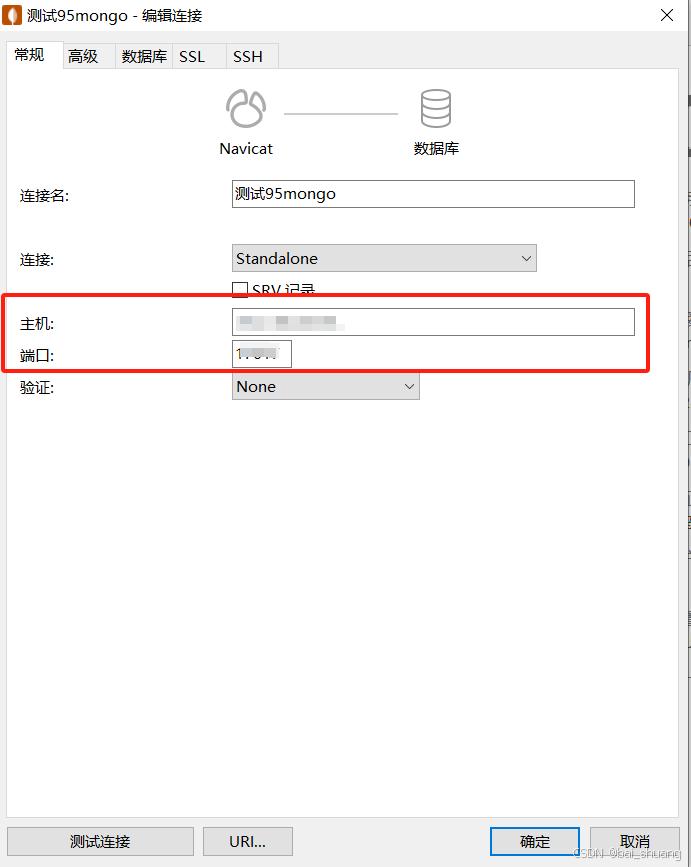
Linux(不同版本系统包含Ubuntu)下安装mongodb详细教程
一、下载MongoDB 在MongoDB官网下载对应的MongoDB版本,可以点击以下链接快速跳转到下载页面: mongodb官网下载地址 注意选择和自己操作系统一致的platform,可以先查看自己的操作系统 查看操作系统详情 命令: uname -a 如图:操…...
如何扫描HTTP代理:步骤与注意事项
HTTP代理是一个复杂的过程,通常用于寻找可用的代理服务器,以便在网络中实现匿名或加速访问。虽然这个过程可以帮助用户找到适合的代理,但也需要注意合法性和道德问题。本文将介绍如何扫描HTTP代理,并提供一些建议和注意事项。 什…...

【分布式微服务云原生】gRPC与Dubbo:分布式服务通信框架的双雄对决
目录 引言gRPC:Google的高性能RPC框架gRPC通信流程图 Dubbo:阿里巴巴的微服务治理框架Dubbo服务治理流程图 表格:gRPC与Dubbo的比较结论呼吁行动Excel表格:gRPC与Dubbo特性总结 摘要 在构建分布式系统时,选择合适的服务…...

Python | Leetcode Python题解之第450题删除二叉搜索树中的节点
题目: 题解: class Solution:def deleteNode(self, root: Optional[TreeNode], key: int) -> Optional[TreeNode]:cur, curParent root, Nonewhile cur and cur.val ! key:curParent curcur cur.left if cur.val > key else cur.rightif cur i…...
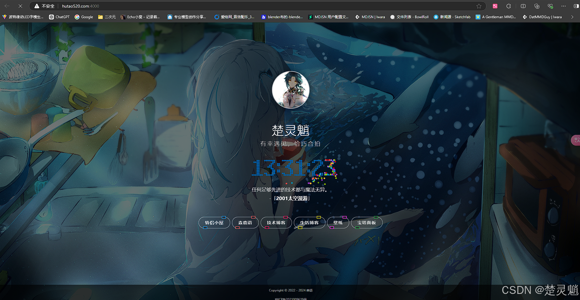
[Linux]从零开始的网站搭建教程
一、谁适合本次教程 学习Linux已经有一阵子了,相信大家对LInux都有一定的认识。本次教程会教大家如何在Linux中搭建一个自己的网站并且实现内网访问。这里我们会演示在Windows中和在Linux中如何搭建自己的网站。当然,如果你没有Linux的基础,这…...
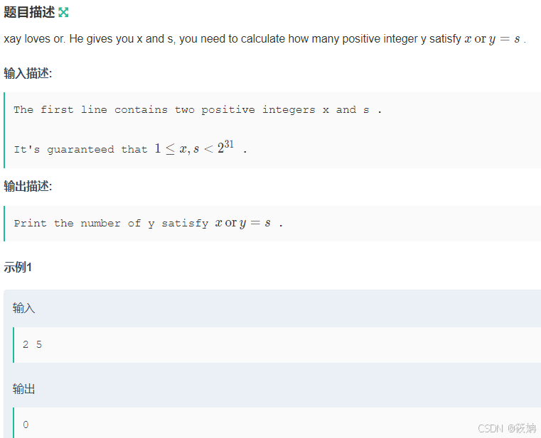
牛客——xay loves or与 __builtin_popcount的使用
xay loves or 题目描述 登录—专业IT笔试面试备考平台_牛客网 运行思路 题目要求我们计算有多少个正整数 yy 满足条件 x \text{ OR } y sx OR ys。这里的“OR”是指按位或运算。为了理解这个问题,我们需要考虑按位或运算的性质。 对于任意两个位 a_iai 和 b_…...
Docker学习和部署ry项目
文章目录 停止Docker重启设置开机自启执行docker ps命令,如果不报错,说明安装启动成功2.然后查看数据卷结果3.查看数据卷详情结果4.查看/var/lib/docker/volumes/html/_data目录可以看到与nginx的html目录内容一样,结果如下:5.进入…...
)
5分钟搞定YOLOv11模型部署到微信小程序(附完整前后端代码)
5分钟极速部署YOLOv11模型到微信小程序的实战指南 当目标检测遇上微信小程序,会碰撞出怎样的火花?YOLOv11作为当前最前沿的实时目标检测模型,与微信小程序的轻量化特性结合,能够为移动端用户提供即开即用的智能视觉服务。本文将带…...

QwQ-32B开源大模型实战:基于ollama构建教育领域智能助教
QwQ-32B开源大模型实战:基于ollama构建教育领域智能助教 1. 引言:当教育遇上推理大模型 想象一下,你是一名中学数学老师,正在批改学生的作业。你发现一道几何证明题,很多学生都卡在了同一个步骤上。传统的AI助手可能…...

AI应用架构师手记:智能生产调度系统接口自动化测试框架搭建与实践
AI应用架构师手记:智能生产调度系统接口自动化测试框架搭建与实践 一、引言:从一次产线停摆说起 凌晨3点,我被手机铃声惊醒——是客户生产总监的紧急电话:某汽车零部件工厂的智能生产调度系统突然“宕机”,三条产线停摆…...

B站缓存视频转换终极指南:m4s-converter让你轻松保存珍贵内容
B站缓存视频转换终极指南:m4s-converter让你轻松保存珍贵内容 【免费下载链接】m4s-converter 将bilibili缓存的m4s转成mp4(读PC端缓存目录) 项目地址: https://gitcode.com/gh_mirrors/m4/m4s-converter 你是否曾为B站视频下架而烦恼?那些精心收…...

Phi-3-vision-128k-instruct在教育领域的应用:智能批改手写作答的数学题试卷
Phi-3-vision-128k-instruct在教育领域的应用:智能批改手写作答的数学题试卷 1. 智能批改带来的教育革新 想象一下这样的场景:一位数学老师面对50份手写试卷,每份包含10道不同题型的数学题。传统批改方式需要逐题检查步骤和结果,…...
)
【微信小程序】如何优雅地获取用户昵称与头像(兼容性优化指南)
1. 微信小程序获取用户信息的现状与挑战 最近在做一个社区类小程序时,我发现获取用户昵称和头像这个看似简单的功能,在实际开发中会遇到不少坑。特别是随着微信基础库版本的迭代,官方对用户隐私保护越来越严格,获取方式也发生了很…...

TinyNAS WebUI可视化开发:零基础JavaScript调用指南
TinyNAS WebUI可视化开发:零基础JavaScript调用指南 用最简单的方式,让前端开发者快速上手TinyNAS WebUI的检测功能 1. 开篇:为什么前端开发者需要了解TinyNAS? 作为一名前端开发者,你可能经常遇到这样的需求…...

RMBG-2.0惊艳效果展示:婚纱裙摆/婴儿胎发/宠物胡须等极限案例集
RMBG-2.0惊艳效果展示:婚纱裙摆/婴儿胎发/宠物胡须等极限案例集 1. 引言:当抠图遇到极限挑战 你有没有遇到过这样的烦恼?想给心爱的宠物换张背景,结果发现它的胡须和毛发边缘总是处理不干净,要么被切掉一半ÿ…...

Qwen3-32B-Chat跨境电商应用:多语言商品描述、平台规则解读、客服话术生成
Qwen3-32B-Chat跨境电商应用:多语言商品描述、平台规则解读、客服话术生成 1. 跨境电商AI助手解决方案 跨境电商行业面临着多语言沟通、平台规则复杂、客服效率低下等痛点。Qwen3-32B-Chat私有部署镜像为这些挑战提供了智能化解决方案,基于RTX4090D 24…...
)
还在用人工打分评大模型?Dify LLM-as-a-judge已成头部AI Lab标配(附Gartner认证评估框架对照表)
第一章:Dify LLM-as-a-judge 的核心价值与演进逻辑在大模型应用落地日益深入的今天,评估生成质量、对齐人类偏好、实现可复现的迭代优化,已成为产品级AI系统不可回避的核心挑战。Dify 将 LLM-as-a-judge 范式深度融入平台能力层,不…...