梯度(Gradient)和 雅各比矩阵(Jacobian Matrix)的区别和联系:中英双语
雅各比矩阵与梯度:区别与联系
在数学与机器学习中,梯度(Gradient) 和 雅各比矩阵(Jacobian Matrix) 是两个核心概念。虽然它们都描述了函数的变化率,但应用场景和具体形式有所不同。本文将通过深入解析它们的定义、区别与联系,并结合实际数值模拟,帮助读者全面理解两者,尤其是雅各比矩阵在深度学习与大模型领域的作用。
1. 梯度与雅各比矩阵的定义
1.1 梯度(Gradient)
梯度是标量函数(输出是一个标量)的变化率的向量化表示。
设函数 ( f : R n → R f: \mathbb{R}^n \to \mathbb{R} f:Rn→R ),其梯度是一个 ( n n n )-维向量:
∇ f ( x ) = [ ∂ f ∂ x 1 ∂ f ∂ x 2 ⋮ ∂ f ∂ x n ] , \nabla f(x) = \begin{bmatrix} \frac{\partial f}{\partial x_1} \\ \frac{\partial f}{\partial x_2} \\ \vdots \\ \frac{\partial f}{\partial x_n} \end{bmatrix}, ∇f(x)= ∂x1∂f∂x2∂f⋮∂xn∂f ,
表示在每个方向上 ( f f f ) 的变化率。
1.2 雅各比矩阵(Jacobian Matrix)
雅各比矩阵描述了向量函数(输出是一个向量)在输入点的变化率。
设函数 ( f : R n → R m \mathbf{f}: \mathbb{R}^n \to \mathbb{R}^m f:Rn→Rm ),即输入是 ( n n n )-维向量,输出是 ( m m m )-维向量,其雅各比矩阵为一个 ( m × n m \times n m×n ) 的矩阵:
D f ( x ) = [ ∂ f 1 ∂ x 1 ∂ f 1 ∂ x 2 ⋯ ∂ f 1 ∂ x n ∂ f 2 ∂ x 1 ∂ f 2 ∂ x 2 ⋯ ∂ f 2 ∂ x n ⋮ ⋮ ⋱ ⋮ ∂ f m ∂ x 1 ∂ f m ∂ x 2 ⋯ ∂ f m ∂ x n ] . Df(x) = \begin{bmatrix} \frac{\partial f_1}{\partial x_1} & \frac{\partial f_1}{\partial x_2} & \cdots & \frac{\partial f_1}{\partial x_n} \\ \frac{\partial f_2}{\partial x_1} & \frac{\partial f_2}{\partial x_2} & \cdots & \frac{\partial f_2}{\partial x_n} \\ \vdots & \vdots & \ddots & \vdots \\ \frac{\partial f_m}{\partial x_1} & \frac{\partial f_m}{\partial x_2} & \cdots & \frac{\partial f_m}{\partial x_n} \end{bmatrix}. Df(x)= ∂x1∂f1∂x1∂f2⋮∂x1∂fm∂x2∂f1∂x2∂f2⋮∂x2∂fm⋯⋯⋱⋯∂xn∂f1∂xn∂f2⋮∂xn∂fm .
- 每一行是某个标量函数 ( f i ( x ) f_i(x) fi(x) ) 的梯度;
- 雅各比矩阵描述了函数在各输入维度上的整体变化。
2. 梯度与雅各比矩阵的区别与联系
| 方面 | 梯度 | 雅各比矩阵 |
|---|---|---|
| 适用范围 | 标量函数 ( f : R n → R f: \mathbb{R}^n \to \mathbb{R} f:Rn→R ) | 向量函数 ( f : R n → R m f: \mathbb{R}^n \to \mathbb{R}^m f:Rn→Rm ) |
| 形式 | 一个 ( n n n )-维向量 | 一个 ( m × n m \times n m×n ) 的矩阵 |
| 含义 | 表示函数 ( f f f ) 在输入空间的变化率 | 表示向量函数 ( f f f ) 的所有输出分量对所有输入变量的变化率 |
| 联系 | 梯度是雅各比矩阵的特殊情况(当 ( m = 1 m = 1 m=1 ) 时,雅各比矩阵退化为梯度) | 梯度可以看作雅各比矩阵的行之一(当输出是标量时只有一行) |
3. 数值模拟:梯度与雅各比矩阵
示例函数
假设有函数 ( f : R 2 → R 2 \mathbf{f}: \mathbb{R}^2 \to \mathbb{R}^2 f:R2→R2 ),定义如下:
f ( x 1 , x 2 ) = [ x 1 2 + x 2 x 1 x 2 ] . \mathbf{f}(x_1, x_2) = \begin{bmatrix} x_1^2 + x_2 \\ x_1 x_2 \end{bmatrix}. f(x1,x2)=[x12+x2x1x2].
3.1 梯度计算(标量函数场景)
若我们关注第一个输出分量 ( f 1 ( x ) = x 1 2 + x 2 f_1(x) = x_1^2 + x_2 f1(x)=x12+x2 ),则其梯度为:
∇ f 1 ( x ) = [ ∂ f 1 ∂ x 1 ∂ f 1 ∂ x 2 ] = [ 2 x 1 1 ] . \nabla f_1(x) = \begin{bmatrix} \frac{\partial f_1}{\partial x_1} \\ \frac{\partial f_1}{\partial x_2} \end{bmatrix} = \begin{bmatrix} 2x_1 \\ 1 \end{bmatrix}. ∇f1(x)=[∂x1∂f1∂x2∂f1]=[2x11].
3.2 雅各比矩阵计算(向量函数场景)
对整个函数 ( f \mathbf{f} f ),其雅各比矩阵为:
D f ( x ) = [ ∂ f 1 ∂ x 1 ∂ f 1 ∂ x 2 ∂ f 2 ∂ x 1 ∂ f 2 ∂ x 2 ] = [ 2 x 1 1 x 2 x 1 ] . Df(x) = \begin{bmatrix} \frac{\partial f_1}{\partial x_1} & \frac{\partial f_1}{\partial x_2} \\ \frac{\partial f_2}{\partial x_1} & \frac{\partial f_2}{\partial x_2} \end{bmatrix} = \begin{bmatrix} 2x_1 & 1 \\ x_2 & x_1 \end{bmatrix}. Df(x)=[∂x1∂f1∂x1∂f2∂x2∂f1∂x2∂f2]=[2x1x21x1].
3.3 Python 实现
以下代码演示了梯度和雅各比矩阵的数值计算:
import numpy as np# 定义函数
def f(x):return np.array([x[0]**2 + x[1], x[0] * x[1]])# 定义雅各比矩阵
def jacobian_f(x):return np.array([[2 * x[0], 1],[x[1], x[0]]])# 计算梯度和雅各比矩阵
x = np.array([1.0, 2.0])  # 输入点
gradient_f1 = np.array([2 * x[0], 1])  # f1 的梯度
jacobian = jacobian_f(x)  # 雅各比矩阵print("Gradient of f1:", gradient_f1)
print("Jacobian matrix of f:", jacobian)
运行结果:
Gradient of f1: [2. 1.]
Jacobian matrix of f:
[[2. 1.][2. 1.]]
4. 在机器学习和深度学习中的作用
4.1 梯度的作用
在深度学习中,梯度主要用于反向传播。当损失函数是标量时,其梯度指示了参数需要如何调整以最小化损失。例如:
- 对于神经网络的参数 ( θ \theta θ ),损失函数 ( L ( θ ) L(\theta) L(θ) ) 的梯度 ( ∇ L ( θ ) \nabla L(\theta) ∇L(θ) ) 用于优化器(如 SGD 或 Adam)更新参数。
4.2 雅各比矩阵的作用
-
多输出问题
雅各比矩阵用于多任务学习和多输出模型(例如,Transformer 的输出是一个序列,维度为 ( m m m )),描述多个输出对输入的变化关系。 -
对抗样本生成
在对抗攻击中,雅各比矩阵被用来计算输入的小扰动如何同时影响多个输出。 -
深度学习中的 Hessian-Free 方法
雅各比矩阵是二阶优化方法(如 Newton 方法)中的重要组成部分,因为 Hessian 矩阵的计算通常依赖雅各比矩阵。 -
大模型推理与精调
在大语言模型中,雅各比矩阵被用于研究模型对输入扰动的敏感性,或指导精调时的梯度裁剪与更新。
5. 总结
- 梯度 是描述标量函数变化率的向量;
- 雅各比矩阵 是描述向量函数所有输出对输入变化的矩阵;
- 两者紧密相关:梯度是雅各比矩阵的特例。
在机器学习与深度学习中,梯度用于优化,雅各比矩阵在多任务学习、对抗训练和大模型分析中有广泛应用。通过数值模拟,我们可以直观理解它们的区别与联系,掌握它们在实际场景中的重要性。
英文版
Jacobian Matrix vs Gradient: Differences and Connections
In mathematics and machine learning, the gradient and the Jacobian matrix are essential concepts that describe the rate of change of functions. While they are closely related, they serve different purposes and are used in distinct scenarios. This blog will explore their definitions, differences, and connections through examples, particularly emphasizing the Jacobian matrix’s role in deep learning and large-scale models.
1. Definition of Gradient and Jacobian Matrix
1.1 Gradient
The gradient is a vector representation of the rate of change for a scalar-valued function.
For a scalar function ( f : R n → R f: \mathbb{R}^n \to \mathbb{R} f:Rn→R ), the gradient is an ( n n n )-dimensional vector:
∇ f ( x ) = [ ∂ f ∂ x 1 ∂ f ∂ x 2 ⋮ ∂ f ∂ x n ] . \nabla f(x) = \begin{bmatrix} \frac{\partial f}{\partial x_1} \\ \frac{\partial f}{\partial x_2} \\ \vdots \\ \frac{\partial f}{\partial x_n} \end{bmatrix}. ∇f(x)= ∂x1∂f∂x2∂f⋮∂xn∂f .
This represents the direction and magnitude of the steepest ascent of ( f f f ).
1.2 Jacobian Matrix
The Jacobian matrix describes the rate of change for a vector-valued function.
For a vector function ( f : R n → R m \mathbf{f}: \mathbb{R}^n \to \mathbb{R}^m f:Rn→Rm ), where the input is ( n n n )-dimensional and the output is ( m m m )-dimensional, the Jacobian matrix is an ( m × n m \times n m×n ) matrix:
D f ( x ) = [ ∂ f 1 ∂ x 1 ∂ f 1 ∂ x 2 ⋯ ∂ f 1 ∂ x n ∂ f 2 ∂ x 1 ∂ f 2 ∂ x 2 ⋯ ∂ f 2 ∂ x n ⋮ ⋮ ⋱ ⋮ ∂ f m ∂ x 1 ∂ f m ∂ x 2 ⋯ ∂ f m ∂ x n ] . Df(x) = \begin{bmatrix} \frac{\partial f_1}{\partial x_1} & \frac{\partial f_1}{\partial x_2} & \cdots & \frac{\partial f_1}{\partial x_n} \\ \frac{\partial f_2}{\partial x_1} & \frac{\partial f_2}{\partial x_2} & \cdots & \frac{\partial f_2}{\partial x_n} \\ \vdots & \vdots & \ddots & \vdots \\ \frac{\partial f_m}{\partial x_1} & \frac{\partial f_m}{\partial x_2} & \cdots & \frac{\partial f_m}{\partial x_n} \end{bmatrix}. Df(x)= ∂x1∂f1∂x1∂f2⋮∂x1∂fm∂x2∂f1∂x2∂f2⋮∂x2∂fm⋯⋯⋱⋯∂xn∂f1∂xn∂f2⋮∂xn∂fm .
- Each row is the gradient of a scalar function ( f i ( x ) f_i(x) fi(x) );
- The Jacobian matrix encapsulates all partial derivatives of ( f \mathbf{f} f ) with respect to its inputs.
2. Differences and Connections Between Gradient and Jacobian Matrix
| Aspect | Gradient | Jacobian Matrix |
|---|---|---|
| Scope | Scalar function ( f : R n → R f: \mathbb{R}^n \to \mathbb{R} f:Rn→R ) | Vector function ( f : R n → R m f: \mathbb{R}^n \to \mathbb{R}^m f:Rn→Rm ) |
| Form | An ( n n n )-dimensional vector | An ( m × n m \times n m×n ) matrix |
| Meaning | Represents the rate of change of ( f f f ) in the input space | Represents the rate of change of all outputs w.r.t. all inputs |
| Connection | The gradient is a special case of the Jacobian (when ( m = 1 m = 1 m=1 )) | Each row of the Jacobian matrix is a gradient of ( f i ( x ) f_i(x) fi(x) ) |
3. Numerical Simulation: Gradient and Jacobian Matrix
Example Function
Consider the function ( f : R 2 → R 2 \mathbf{f}: \mathbb{R}^2 \to \mathbb{R}^2 f:R2→R2 ) defined as:
f ( x 1 , x 2 ) = [ x 1 2 + x 2 x 1 x 2 ] . \mathbf{f}(x_1, x_2) = \begin{bmatrix} x_1^2 + x_2 \\ x_1 x_2 \end{bmatrix}. f(x1,x2)=[x12+x2x1x2].
3.1 Gradient Computation (Scalar Function Case)
If we focus on the first output component ( f 1 ( x ) = x 1 2 + x 2 f_1(x) = x_1^2 + x_2 f1(x)=x12+x2 ), the gradient is:
∇ f 1 ( x ) = [ ∂ f 1 ∂ x 1 ∂ f 1 ∂ x 2 ] = [ 2 x 1 1 ] . \nabla f_1(x) = \begin{bmatrix} \frac{\partial f_1}{\partial x_1} \\ \frac{\partial f_1}{\partial x_2} \end{bmatrix} = \begin{bmatrix} 2x_1 \\ 1 \end{bmatrix}. ∇f1(x)=[∂x1∂f1∂x2∂f1]=[2x11].
3.2 Jacobian Matrix Computation (Vector Function Case)
For the full vector function ( f \mathbf{f} f ), the Jacobian matrix is:
D f ( x ) = [ ∂ f 1 ∂ x 1 ∂ f 1 ∂ x 2 ∂ f 2 ∂ x 1 ∂ f 2 ∂ x 2 ] = [ 2 x 1 1 x 2 x 1 ] . Df(x) = \begin{bmatrix} \frac{\partial f_1}{\partial x_1} & \frac{\partial f_1}{\partial x_2} \\ \frac{\partial f_2}{\partial x_1} & \frac{\partial f_2}{\partial x_2} \end{bmatrix} = \begin{bmatrix} 2x_1 & 1 \\ x_2 & x_1 \end{bmatrix}. Df(x)=[∂x1∂f1∂x1∂f2∂x2∂f1∂x2∂f2]=[2x1x21x1].
3.3 Python Implementation
The following Python code demonstrates how to compute the gradient and Jacobian matrix numerically:
import numpy as np# Define the function
def f(x):return np.array([x[0]**2 + x[1], x[0] * x[1]])# Define the Jacobian matrix
def jacobian_f(x):return np.array([[2 * x[0], 1],[x[1], x[0]]])# Input point
x = np.array([1.0, 2.0])# Compute the gradient of f1
gradient_f1 = np.array([2 * x[0], 1])  # Gradient of the first output component# Compute the Jacobian matrix
jacobian = jacobian_f(x)print("Gradient of f1:", gradient_f1)
print("Jacobian matrix of f:", jacobian)
Output:
Gradient of f1: [2. 1.]
Jacobian matrix of f:
[[2. 1.][2. 1.]]
4. Applications in Machine Learning and Deep Learning
4.1 Gradient Applications
In deep learning, the gradient is critical for backpropagation. When the loss function is a scalar, its gradient indicates how to adjust the parameters to minimize the loss. For example:
- For a neural network with parameters ( θ \theta θ ), the loss function ( L ( θ ) L(\theta) L(θ) ) has a gradient ( ∇ L ( θ ) \nabla L(\theta) ∇L(θ) ), which is used by optimizers (e.g., SGD, Adam) to update the parameters.
4.2 Jacobian Matrix Applications
-
Multi-Output Models
The Jacobian matrix is essential for multi-task learning or models with multiple outputs (e.g., transformers where the output is a sequence). It describes how each input affects all outputs. -
Adversarial Examples
In adversarial attacks, the Jacobian matrix helps compute how small perturbations in input affect multiple outputs simultaneously. -
Hessian-Free Methods
In second-order optimization methods (e.g., Newton’s method), the Jacobian matrix is used to compute the Hessian matrix, which is crucial for convergence. -
Large Model Fine-Tuning
For large language models, the Jacobian matrix is used to analyze how sensitive a model is to input perturbations, guiding techniques like gradient clipping or parameter-efficient fine-tuning (PEFT).
5. Summary
- The gradient is a vector describing the rate of change of a scalar function, while the Jacobian matrix is a matrix describing the rate of change of a vector function.
- The gradient is a special case of the Jacobian matrix (when there is only one output dimension).
- In machine learning, gradients are essential for optimization, whereas Jacobian matrices are widely used in multi-output models, adversarial training, and fine-tuning large models.
Through numerical simulations and real-world applications, understanding the gradient and Jacobian matrix can significantly enhance your knowledge of optimization, deep learning, and large-scale model analysis.
后记
2024年12月19日15点30分于上海,在GPT4o大模型辅助下完成。
相关文章:
和 雅各比矩阵(Jacobian Matrix)的区别和联系:中英双语)
梯度(Gradient)和 雅各比矩阵(Jacobian Matrix)的区别和联系:中英双语
雅各比矩阵与梯度:区别与联系 在数学与机器学习中,梯度(Gradient) 和 雅各比矩阵(Jacobian Matrix) 是两个核心概念。虽然它们都描述了函数的变化率,但应用场景和具体形式有所不同。本文将通过…...

Vscode搭建C语言多文件开发环境
一、文章内容简介 本文介绍了 “Vscode搭建C语言多文件开发环境”需要用到的软件,以及vscode必备插件,最后多文件编译时tasks.json文件和launch.json文件的配置。即目录顺序。由于内容较多,建议大家在阅读时使用电脑阅读,按照目录…...

自定义 C++ 编译器的调用与管理
在 C 项目中,常常需要自动化地管理编译流程,例如使用 MinGW 或 Visual Studio 编译器进行代码的编译和链接。为了方便管理不同编译器和简化编译流程,我们开发了一个 CompilerManager 类,用于抽象编译器的查找、命令生成以及执行。…...
时间管理系统|Java|SSM|JSP|
【技术栈】 1⃣️:架构: B/S、MVC 2⃣️:系统环境:Windowsh/Mac 3⃣️:开发环境:IDEA、JDK1.8、Maven、Mysql5.7 4⃣️:技术栈:Java、Mysql、SSM、Mybatis-Plus、JSP、jquery,html 5⃣️数据库可…...

用SparkSQL和PySpark完成按时间字段顺序将字符串字段中的值组合在一起分组显示
用SparkSQL和PySpark完成以下数据转换。 源数据: userid,page_name,visit_time 1,A,2021-2-1 2,B,2024-1-1 1,C,2020-5-4 2,D,2028-9-1 目的数据: user_id,page_name_path 1,C->A 2,B->D PySpark: from pyspark.sql import SparkSes…...
Sentinel 学习笔记3-责任链与工作流程
本文属于sentinel学习笔记系列。网上看到吴就业老师的专栏,原文地址如下: https://blog.csdn.net/baidu_28523317/category_10400605.html 上一篇梳理了概念与核心类:Sentinel 学习笔记2- 概念与核心类介绍-CSDN博客 补一个点:…...
Latex 转换为 Word(使用GrindEQ )(英文转中文,毕业论文)
效果预览 第一步: 告诉chatgpt: 将latex格式中的英文翻译为中文(符号和公式不要动),给出latex格式第二步: Latex 转换为 Word(使用GrindEQ ) 视频 https://www.bilibili.com/video/BV1f242…...

使用Chat-LangChain模块创建一个与用户交流的机器人
当然!要使用Chat-LangChain模块创建一个与用户交流的机器人,你需要安装并配置一些Python库。以下是一个基本的步骤指南和示例代码,帮助你快速上手。 安装依赖库 首先,你需要安装langchain库,它是一个高级框架&#x…...

国家认可的人工智能从业人员证书如何报考?
一、证书出台背景 为进一步贯彻落实中共中央印发《关于深化人才发展体制机制改革的意见》和国务院印发《关于“十四五”数字经济发展规划》等有关工作的部署要求,深入实施人才强国战略和创新驱动发展战略,加强全国数字化人才队伍建设,持续推…...

【网络云计算】2024第51周-每日【2024/12/17】小测-理论-解析
文章目录 1. 计算机网络有哪些分类2. 计算机网络中协议与标准的区别3. 计算机网络拓扑有哪些结构4. 常用的网络设备有哪些,分属于OSI的哪一层5. IEEE802局域网标准有哪些 【网络云计算】2024第51周-每日【2024/12/17】小测-理论-解析 1. 计算机网络有哪些分类 计算…...
每日十题八股-2024年12月19日
1.Bean注入和xml注入最终得到了相同的效果,它们在底层是怎样做的? 2.Spring给我们提供了很多扩展点,这些有了解吗? 3.MVC分层介绍一下? 4.了解SpringMVC的处理流程吗? 5.Handlermapping 和 handleradapter有…...
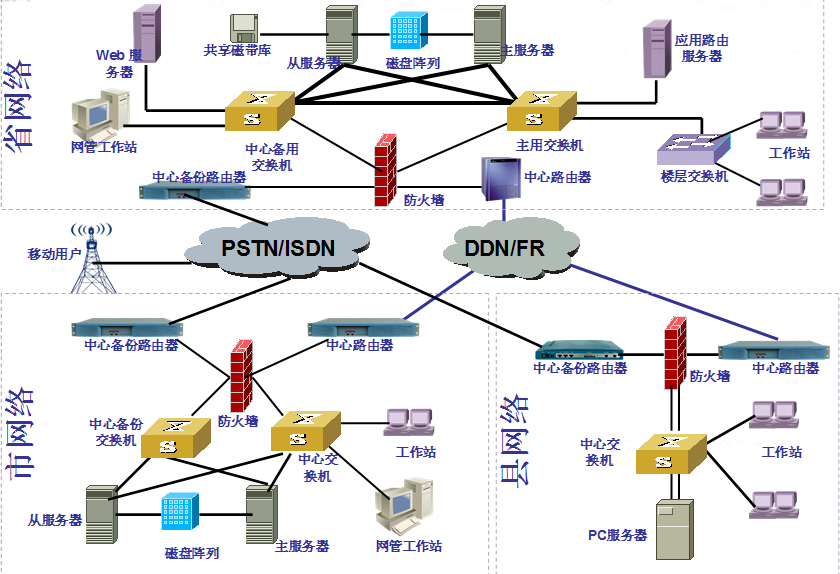
网络方案设计
一、网络方案设计目标 企业网络系统的构成 应用软件 计算平台 物理网络及拓扑结构 网络软件及工具软件 网络互连设备 广域网连接 无论是复杂的,还是简单的计算机网络,都包括了以下几个基本元素 : 应用软件----支持用户完成专门操作的软件。…...

学习记录:electron主进程与渲染进程直接的通信示例【开箱即用】
electron主进程与渲染进程直接的通信示例 1. 背景: electronvue实现桌面应用开发 2.异步模式 2.1使用.send 和.on的方式 preload.js中代码示例: const { contextBridge, ipcRenderer} require(electron);// 暴露通信接口 contextBridge.exposeInMa…...

【Java数据结构】ArrayList类
List接口 List是一个接口,它继承Collection接口,Collection接口中的一些常用方法 List也有一些常用的方法。List是一个接口,它并不能直接实例化,ArrayList和LinkedList都实现了List接口,它们的常用方法都很相似。 Ar…...
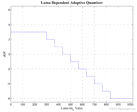
HDR视频技术之十:MPEG 及 VCEG 的 HDR 编码优化
与传统标准动态范围( SDR)视频相比,高动态范围( HDR)视频由于比特深度的增加提供了更加丰富的亮区细节和暗区细节。最新的显示技术通过清晰地再现 HDR 视频内容使得为用户提供身临其境的观看体验成为可能。面对目前日益…...
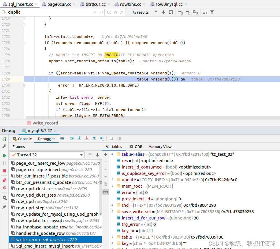
71 mysql 中 insert into ... on duplicate key update ... 的实现
前言 这个也是我们经常可能会使用到的相关的特殊语句 当插入数据存在 唯一索引 或者 主键索引 相关约束的时候, 如果存在 约束冲突, 则更新目标记录 这个处理是类似于 逻辑上的 save 操作 insert into tz_test_02 (field1, field2) values (field11, 11) on duplicate …...
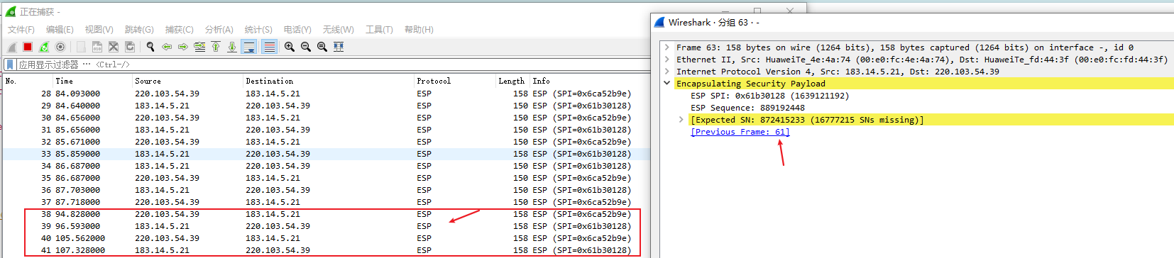
计算机网络-GRE Over IPSec实验
一、概述 前情回顾:上次基于IPsec VPN的主模式进行了基础实验,但是很多高级特性没有涉及,如ike v2、不同传输模式、DPD检测、路由方式引入路由、野蛮模式等等,以后继续学习吧。 前面我们已经学习了GRE可以基于隧道口实现分支互联&…...
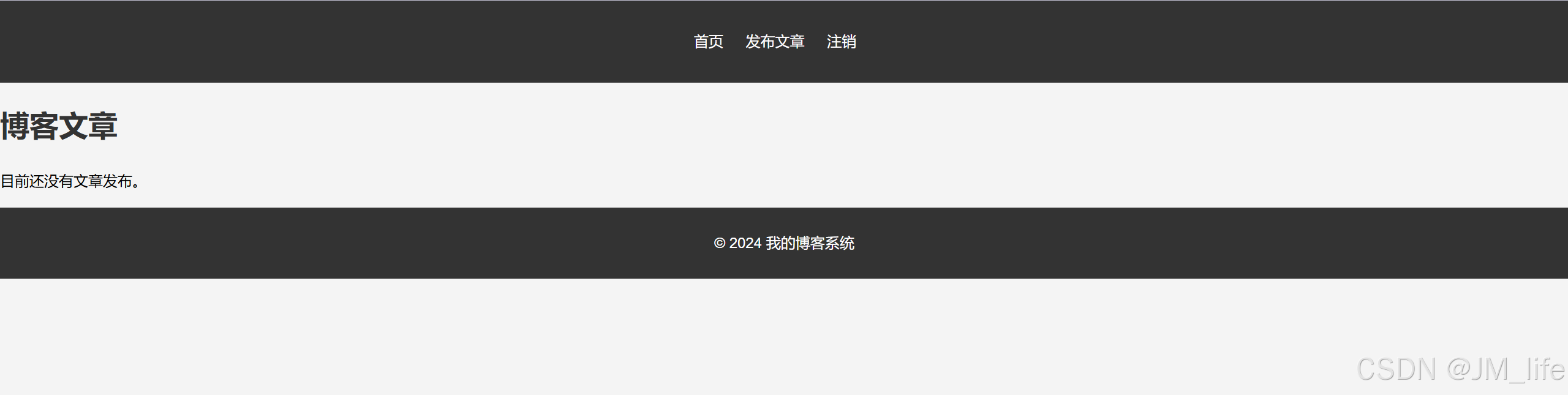
你的第一个博客-第一弹
使用 Flask 开发博客 Flask 是一个轻量级的 Web 框架,适合小型应用和学习项目。我们将通过 Flask 开发一个简单的博客系统,支持用户注册、登录、发布文章等功能。 步骤: 安装 Flask 和其他必要库: 在开发博客之前,首…...

若依启动项目时配置为 HTTPS 协议
文章目录 1、需求提出2、应用场景3、解决思路4、注意事项5、完整代码第一步:修改 vue.config.js 文件第二步:运行项目第三步:处理浏览器警告 6、运行结果 1、需求提出 在开发本地项目时,默认启动使用的是 HTTP 协议。但在某些测试…...
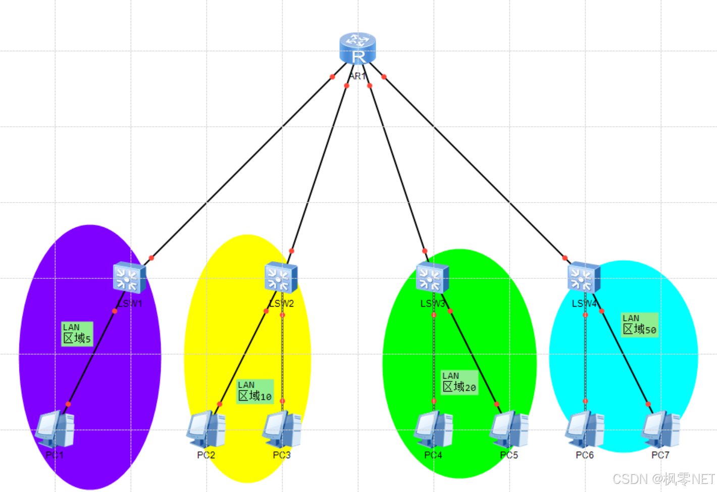
学习思考:一日三问(学习篇)之匹配VLAN
学习思考:一日三问(学习篇)之匹配VLAN 一、学了什么(是什么)1.1 理解LAN与"V"的LAN1.2 理解"V"的LAN怎么还原成LAN1.3 理解二层交换机眼中的"V"的LAN 二、为何会产生需求(为…...

告别臃肿:Win11Debloat让你的Windows 11系统焕然一新
告别臃肿:Win11Debloat让你的Windows 11系统焕然一新 【免费下载链接】Win11Debloat A simple, lightweight PowerShell script that allows you to remove pre-installed apps, disable telemetry, as well as perform various other changes to declutter and cus…...

论完善代码版本信息构建AI在精工产业与智能设备短板—东方仙盟
出众的现代 AI时至今日,人工智能发展日新月异。在 UI 设计、网页开发、纯软件系统搭建等不依托实体硬件的领域,AI 表现已然成熟。常规信息化工作,AI 皆可独立完成,效率出众,为日常开发与设计减负良多。精工硬件领域 AI…...

RuoYi-Vue-Plus项目实战:用WebSocket实现‘服务端通知’功能,我踩了这些坑
RuoYi-Vue-Plus实战:WebSocket服务端通知功能深度解析与避坑指南 在当今企业级应用开发中,实时通信已成为提升用户体验的关键要素。当产品经理提出"后台操作成功时前端实时弹窗提示"的需求时,作为技术负责人的你该如何选择技术方案…...

FLUX.1-dev FP8低显存优化版终极指南:破解大模型部署难题
FLUX.1-dev FP8低显存优化版终极指南:破解大模型部署难题 【免费下载链接】flux1-dev 项目地址: https://ai.gitcode.com/hf_mirrors/Comfy-Org/flux1-dev 在AI图像生成领域,显存限制一直是开发者面临的核心挑战。当主流模型动辄需要24GB以上显存…...

Real-ESRGAN终极指南:5分钟掌握AI图像超分辨率技术,让模糊照片秒变高清
Real-ESRGAN终极指南:5分钟掌握AI图像超分辨率技术,让模糊照片秒变高清 【免费下载链接】Real-ESRGAN Real-ESRGAN aims at developing Practical Algorithms for General Image/Video Restoration. 项目地址: https://gitcode.com/gh_mirrors/re/Real…...

终极指南:如何用OpenHTMLtoPDF轻松生成专业级PDF文档
终极指南:如何用OpenHTMLtoPDF轻松生成专业级PDF文档 【免费下载链接】openhtmltopdf An HTML to PDF library for the JVM. Based on Flying Saucer and Apache PDF-BOX 2. With SVG image support. Now also with accessible PDF support (WCAG, Section 508, PDF…...

ComfyUI InstantID终极指南:3步实现人脸完美保留的AI图像生成
ComfyUI InstantID终极指南:3步实现人脸完美保留的AI图像生成 【免费下载链接】ComfyUI_InstantID 项目地址: https://gitcode.com/gh_mirrors/co/ComfyUI_InstantID 你是否曾经尝试过用AI生成图像,却发现生成的人物完全不像你想要的参考对象&am…...

终极游戏光标解决方案:YoloMouse让你的鼠标在游戏中清晰可见
终极游戏光标解决方案:YoloMouse让你的鼠标在游戏中清晰可见 【免费下载链接】YoloMouse Game Cursor Changer 项目地址: https://gitcode.com/gh_mirrors/yo/YoloMouse 你是否曾在激烈的游戏战斗中迷失了鼠标光标?当屏幕上特效绚烂、技能乱飞时&…...

UV-UI框架终极指南:如何快速构建跨平台应用
UV-UI框架终极指南:如何快速构建跨平台应用 【免费下载链接】uv-ui uv-ui 破釜沉舟之兼容vue32、app、h5、小程序等多端基于uni-app和uView2.x的生态框架,支持单独导入,开箱即用,利剑出击。 项目地址: https://gitcode.com/gh_m…...

Buck电路纹波太大?可能是你的电容和ESR没选对!三种RC场景下的实战分析与选型指南
Buck电路纹波优化实战:电容与ESR选型的三维决策框架 实验室里示波器屏幕上那条本该平滑的直流输出波形,此刻却像心电图般剧烈起伏——这是每位电源工程师都经历过的"纹波焦虑"时刻。当我们面对Buck电路输出纹波超标问题时,传统定性…...