【TI毫米波雷达】DCA1000不使用mmWave Studio的数据采集方法,以及自动化实时数据采集
【TI毫米波雷达】DCA1000不使用mmWave Studio的数据采集方法,以及自动化实时数据采集
mmWave Studio提供的功能完全够用了 不用去纠结用DCA1000低延迟、无GUI传数据 速度最快又保证算力无非就是就是Linux板自己写驱动做串口和UDP 做雷达产品应用也不会采用DCA1000的方案 有这时间不如研究一下TI驱动如何写!
文章目录
- 前言
- DCA1000配置(IWR6843AOP为例)
- 开发板硬件配置
- DCA1000硬件配置
- mmWave Studio数据采集
- 环境
- 配置
- Connection
- StaticCongfig
- DataConfig
- SensorConfig
- 报错解决方案
- 实时采集
- 不使用mmWave Studio进行数据采集
- DCA1000的控制
- 雷达板的控制
- 实时采集
- 附录:结构框架
- 雷达基本原理叙述
- 雷达天线排列位置
- 芯片框架
- Demo工程功能
- CCS工程导入
- 工程叙述
- Software Tasks
- Data Path
- Output information sent to host
- List of detected objects
- Range profile
- Azimuth static heatmap
- Azimuth/Elevation static heatmap
- Range/Doppler heatmap
- Stats information
- Side information of detected objects
- Temperature Stats
- Range Bias and Rx Channel Gain/Phase Measurement and Compensation
- Streaming data over LVDS
- Implementation Notes
- How to bypass CLI
- Hardware Resource Allocation
前言
碰到不止一个问我用DCA1000做毕设的了
一般都是导师给的任务 如图:

sar雷达成像就不说了 更有甚者 做个目标识别 人员计数还要用DCA1000?
【TI毫米波雷达】雷达开发入门浅谈,为什么说用DCA1000做毕设要延毕?(以IWR6843AOP为例)
DCA1000是毫米波雷达初期开发时 不熟悉TI生态 用来采集数据、仿真使用的
只能配合开发板和官方的mmWave Studio软件使用
输出的数据都帮你做好了数据解析、信号处理等步骤
可以做到完全不用写一行代码就实现毫米波雷达的射频配置仿真
另外 也可以拿原始数据做MATLAB数据处理、算法仿真
但在应用方面 完全无法胜任实时性
若要做到产品应用的实时性要求 必须在设计好射频、算法后 将这部分移植到TI毫米波雷达生态中 采用CCS进行毫米波雷达开发 再将代码烧录雷达里面!!!
如果你的导师真的要你用DCA1000做毕设 要么就是导师太蠢完全不懂雷达 要么就是没有产品应用的实时性要求 只有算法仿真要求 如果是后者 问清楚 随便应付一下就得了
如果非要用DCA1000开发 那么可以看后文
DCA1000配置(IWR6843AOP为例)
开发板硬件配置
IWR6843AOPEVM-G版本可以直接与DCA1000EVM连接 进行数据获取
不需要连接MMWAVEICBOOST版
直接使用 DCA1000+mmWave Studio 软件进行数据采集
在官方手册中 User’s Guide 60GHz 毫米波传感器EVM 有相关模式的开关配置 但其实是错的

应采用如下ti上的配置:


dev.ti.com/tirex/explore/node?a=VLyFKFf__4.12.0&node=A__AGTrhNYW8jE6cMxbovlfaA__com.ti.mmwave_industrial_toolbox__VLyFKFf__4.12.0
DCA1000和软件使用方法参考手册 ZHCAB69-12.2021 使用低速串行总线的实时ADC原始数据采集方法
DCA1000硬件配置
DCA1000的硬件配置看这个手册 SPRUIK7-05.2018 DCA1000EVM Quick Start Guide

尤其要注意配置静态IP地址:

IWR6843AOPEVM不需要连串口线 但要连供电线
其实 IWR6843AOPEVM的开关就是要路由到60pin的引脚那里

官方文档错误很多
另外 在使用IWR6843AOPEVM-G的DCA1000EVM模式时 电脑上的端口是没有XDS的 这一点手册也不符合

调试好后 在打开mmWave Studio软件就像数据获取就好了
如果硬件配置成功 则可以通过mmWave Studio的Output看到配置信息

mmWave Studio数据采集
硬件方面连接好以后 就可以打开mmWave Studio了
环境
需要安装mmWave SDK
以及MATLAB runtime
是运行项目所需要的库,没装它项目会运行不了
ww2.mathworks.cn/products/compiler/matlab-runtime.html
最新版可能有bug
推荐下载安装MCR_R2015aSP1_win32_installer.exe
in.mathworks.com/supportfiles/downloads/R2015a/deployment_files/R2015aSP1/installers/win32/MCR_R2015aSP1_win32_installer.exe
配置
如果硬件配置成功 则可以通过mmWave Studio的Output看到配置信息
按照如图步骤 在radar api里面一步步来操作
Connection

其中 RS232选择波特率115200 enhanced端口
BSS FW在路径:
D:\TI_SDK\mmwave_studio_02_01_01_00\rf_eval_firmware\radarss
MSS FW在:
D:\TI_SDK\mmwave_studio_02_01_01_00\rf_eval_firmware\masterss
选择好以后 点击加载
最后再点击SPI连接
其中 雷达频率选择60GHz
连上以后:


StaticCongfig
按照蓝色按钮标记,根据自己需求 更改参数配置,并一一点击set按钮配置。

DataConfig

SensorConfig

按提示配置完参数后即可开始采集。
首先点击1️⃣DCA1000ARM,其实点击2️⃣Trigger Frame 便开始对雷达数据进行采集,最后采集完成,点击3️⃣PostProc便可查看雷达的数据处理后的效果图。采集到的原始数据存在4️⃣adc_data.bin文件中。
若没有数据产生 则肯定是没有连接到DCA1000ARM 需要点击左侧的SetUp DCA1000进行连接 同时 防火墙权限开到最大 或者干脆关闭防火墙
在进行第一步后 建议等待两秒再开始采集
tirrger frame就是开始采集 stop frame就是停止采集
生成的bin文件大小由配置决定 但数据由采集场景和时间等决定

雷达数据:

生成的数据:

报错解决方案
连接DCA1000时 Output报错 无法读取FPGA版本号等数据
Timeout Error! System disconnected
这是在连接FPGA时报错 网口的问题 防火墙设置为专用和公用网络都运行
或者IP没配置好
或者直接关闭防火墙
或者换个网口
连接SPI时报错 Output报错
MSS Power Up async event was not received!
检查DCA1000供电
将板子用UniFlash擦除后重连
或板子没有将开关设置为SPI模式 设置一下
实时采集
有两种方案:
- 配置雷达帧数尽可能少 并开启雷达 在采集过程中 不断生成bin文件 并且不断进行bin文件的解析和处理
- 配置雷达帧数尽可能多(或者无限) 并开启雷达 在采集过程中 不断对UDP协议进行抓包 并进行解析
这两种实时采集的方法 都离不开对mmWave Studio的lua脚本编写


在mmWave Studio中可以导入lua脚本
另外 相关配置也可以通过csv文件进行保存和读取

重点在于frame配置

No of Frames表示一次采集多少帧
如果用方法1 则可以配置为10帧、20帧皆可(大约1s)
也就是每1s生成一次bin文件 并进行一次解析 或者每隔几秒钟生成一次都行
如果用方法2 则可以根据需求配置为512帧以上(或为0 表示一直进行下去)
512帧算下来至少就是20s 可以根据实际需求进行配置
通过Trigger Frame开启采集 在采集过程中 即可通过UDP解包来完成实时数据获取和解析
不使用mmWave Studio进行数据采集
其实可以直接通过串口控制DCA1000和雷达 但但官方也提供了API接口应用程序 则可以直接使用shell脚本进行操作
DCA1000的控制
官方提供了DCA1000的API接口
即:
DCA1000EVM_CLI_Control.exe
通过该exe程序 可以将json脚本传递给DCA1000 并自动进行雷达配置
通过文档可以查看使用方法:
TI_DCA1000EVM_CLI_Software_UserGuide.pdf
在此程序目录下通过cmd调用:
DCA1000EVM_CLI_Control.exe fpga cf.json
DCA1000EVM_CLI_Control.exe record cf.json
DCA1000EVM_CLI_Control.exe start_record cf.json
即打开cf.json的fpga配置文件
打开cf.json的记录配置文件
打开cf.json的开启配置文件
整体的配置文件为cf.json 原路径为C:\ti\mmwave_studio_02_01_01_00\mmWaveStudio\PostProc可以根据自己的需求来进行修改操作
DCA1000开始监听数据 如果此时雷达开始工作 DCA1000便会开始采集数据
雷达板的控制
随便烧录一个雷达的out_of_box工程进去 然后通过串口或者官方的开箱测试GUI使用CLI指令将雷达的配置发送
并且确保开启sensorStart之前 DCA1000开启了数据监听
实时采集
通过shell脚本等方法进行自动化数据采集后 即可通过上一章节中的任一方法进行实时采集
附录:结构框架
雷达基本原理叙述
雷达工作原理是上电-发送chirps-帧结束-处理-上电循环
一个Frame,首先是信号发送,比如96个chirp就顺次发出去,然后接收回来,混频滤波,ADC采样,这些都是射频模块的东西。射频完成之后,FFT,CFAR,DOA这些就是信号处理的东西。然后输出给那个结构体,就是当前帧获得的点云了。

在射频发送阶段 一个frame发送若干个chirp 也就是上图左上角
第一个绿色点为frame start 第二个绿色点为frame end
其中发送若干chirps(小三角形)
chirps的个数称为numLoops(代码中 rlFrameCfg_t结构体)
在mmwave studio上位机中 则称为 no of chirp loops
frame end 到 周期结束的时间为计算时间 称为inter frame period

frame start到循环结束的时间称为framePeriodicity(代码中 rlFrameCfg_t结构体)
在mmwave studio上位机中 则称为 Periodicity
如下图frame配置部分

在inter frame Periodicity时间内(比如这里整个周期是55ms)
就是用于计算和处理的时间 一定比55ms要小
如果chirps很多的话 那么计算时间就会减小
如果是处理点云数据 则只需要每一帧计算一次点云即可
计算出当前帧的xyz坐标和速度 以及保存时间戳
雷达天线排列位置
在工业雷达包:
C:\ti\mmwave_industrial_toolbox_4_12_0\antennas\ant_rad_patterns
路径下 有各个EVM开发板的天线排列说明
同样的 EVM手册中也有
如IWR6843AOPEVM:


其天线的间距等等位于数据手册:

芯片框架
IWR6843AOP可以分成三个主要部分及多个外设
BSS:雷达前端部分
MSS:cortex-rf4内核 主要用于控制
DSS: DSP C674内核 主要用于信号处理
外设:UART GPIO DPM HWA等

其中 大部分外设可以被MSS或DSS调用
另外 雷达前端BSS部分在SDK里由MMWave API调用
代码框架上 可以分成两个代码 MSS和DSS 两个代码同时运行 通过某些外设进行同步 协同运作
但也可以只跑一个内核 在仅MSS模式下 依旧可以调用某些用于信号处理的外设 demo代码就是如此
如下图为demo代码流程

Demo工程功能
IWR6843AOP的开箱工程是根据IWR6843AOPEVM开发板来的
该工程可以将IWR6843AOP的两个串口利用起来 实现的功能主要是两个方面:
通过115200波特率的串口配置参数 建立握手协议
通过115200*8的串口输出雷达数据
此工程需要匹配TI官方的上位机:mmWave_Demo_Visualizer_3.6.0来使用
该上位机可以在连接串口后自动化操作 并且对雷达数据可视化


关于雷达参数配置 则在SDK的mmw\profiles目录下
言简意赅 可以直接更改该目录下的文件参数来达到配置雷达参数的目的

但这种方法不利于直接更改 每次用上位机运行后的参数是固定的(上位机运行需要SDK环境) 所以也可以在代码中写死 本文探讨的就是这个方向
CCS工程导入
首先 在工业雷达包目录下找到该工程设置
C:\ti\mmwave_industrial_toolbox_4_12_0\labs\Out_Of_Box_Demo\src\xwr6843AOP
使用CCS的import project功能导入工程后 即可完成环境搭建

这里用到的SDK最新版为3.6版本
工程叙述
以下来自官方文档 可以直接跳过
Software Tasks
The demo consists of the following (SYSBIOS) tasks:
MmwDemo_initTask. This task is created/launched by main and is a one-time active task whose main functionality is to initialize drivers (<driver>_init), MMWave module (MMWave_init), DPM module (DPM_init), open UART and data path related drivers (EDMA, HWA), and create/launch the following tasks (the CLI_task is launched indirectly by calling CLI_open).
CLI_task. This command line interface task provides a simplified 'shell' interface which allows the configuration of the BSS via the mmWave interface (MMWave_config). It parses input CLI configuration commands like chirp profile and GUI configuration. When sensor start CLI command is parsed, all actions related to starting sensor and starting the processing the data path are taken. When sensor stop CLI command is parsed, all actions related to stopping the sensor and stopping the processing of the data path are taken
MmwDemo_mmWaveCtrlTask. This task is used to provide an execution context for the mmWave control, it calls in an endless loop the MMWave_execute API.
MmwDemo_DPC_ObjectDetection_dpmTask. This task is used to provide an execution context for DPM (Data Path Manager) execution, it calls in an endless loop the DPM_execute API. In this context, all of the registered object detection DPC (Data Path Chain) APIs like configuration, control and execute will take place. In this task. When the DPC's execute API produces the detected objects and other results, they are transmitted out of the UART port for display using the visualizer.
Data Path

Top Level Data Path Processing Chain

Top Level Data Path Timing
The data path processing consists of taking ADC samples as input and producing detected objects (point-cloud and other information) to be shipped out of UART port to the PC. The algorithm processing is realized using the DPM registered Object Detection DPC. The details of the processing in DPC can be seen from the following doxygen documentation:
ti/datapath/dpc/objectdetection/objdethwa/docs/doxygen/html/index.html
Output information sent to host
Output packets with the detection information are sent out every frame through the UART. Each packet consists of the header MmwDemo_output_message_header_t and the number of TLV items containing various data information with types enumerated in MmwDemo_output_message_type_e. The numerical values of the types can be found in mmw_output.h. Each TLV item consists of type, length (MmwDemo_output_message_tl_t) and payload information. The structure of the output packet is illustrated in the following figure. Since the length of the packet depends on the number of detected objects it can vary from frame to frame. The end of the packet is padded so that the total packet length is always multiple of 32 Bytes.

Output packet structure sent to UART
The following subsections describe the structure of each TLV.
List of detected objects
Type: (MMWDEMO_OUTPUT_MSG_DETECTED_POINTS)Length: (Number of detected objects) x (size of DPIF_PointCloudCartesian_t)Value: Array of detected objects. The information of each detected object is as per the structure DPIF_PointCloudCartesian_t. When the number of detected objects is zero, this TLV item is not sent. The maximum number of objects that can be detected in a sub-frame/frame is DPC_OBJDET_MAX_NUM_OBJECTS.The orientation of x,y and z axes relative to the sensor is as per the following figure. (Note: The antenna arrangement in the figure is shown for standard EVM (see gAntDef_default) as an example but the figure is applicable for any antenna arrangement.)

Coordinate Geometry
The whole detected objects TLV structure is illustrated in figure below.

Detected objects TLV
Range profile
Type: (MMWDEMO_OUTPUT_MSG_RANGE_PROFILE)Length: (Range FFT size) x (size of uint16_t)Value: Array of profile points at 0th Doppler (stationary objects). The points represent the sum of log2 magnitudes of received antennas expressed in Q9 format.Noise floor profile
Type: (MMWDEMO_OUTPUT_MSG_NOISE_PROFILE)Length: (Range FFT size) x (size of uint16_t)Value: This is the same format as range profile but the profile is at the maximum Doppler bin (maximum speed objects). In general for stationary scene, there would be no objects or clutter at maximum speed so the range profile at such speed represents the receiver noise floor.
Azimuth static heatmap
Type: (MMWDEMO_OUTPUT_MSG_AZIMUT_STATIC_HEAT_MAP)Length: (Range FFT size) x (Number of "azimuth" virtual antennas) (size of cmplx16ImRe_t_)Value: Array DPU_AoAProcHWA_HW_Resources::azimuthStaticHeatMap. The antenna data are complex symbols, with imaginary first and real second in the following order:
Imag(ant 0, range 0), Real(ant 0, range 0),...,Imag(ant N-1, range 0),Real(ant N-1, range 0)...Imag(ant 0, range R-1), Real(ant 0, range R-1),...,Imag(ant N-1, range R-1),Real(ant N-1, range R-1)
Note that the number of virtual antennas is equal to the number of “azimuth” virtual antennas. The antenna symbols are arranged in the order as they occur at the input to azimuth FFT. Based on this data the static azimuth heat map could be constructed by the GUI running on the host.
Azimuth/Elevation static heatmap
Type: (MMWDEMO_OUTPUT_MSG_AZIMUT_ELEVATION_STATIC_HEAT_MAP)Length: (Range FFT size) x (Number of all virtual antennas) (size of cmplx16ImRe_t_)Value: Array DPU_AoAProcHWA_HW_Resources::azimuthStaticHeatMap. The antenna data are complex symbols, with imaginary first and real second in the following order:
Imag(ant 0, range 0), Real(ant 0, range 0),...,Imag(ant N-1, range 0),Real(ant N-1, range 0)...Imag(ant 0, range R-1), Real(ant 0, range R-1),...,Imag(ant N-1, range R-1),Real(ant N-1, range R-1)
Note that the number of virtual antennas is equal to the total number of active virtual antennas. The antenna symbols are arranged in the order as they occur in the radar cube matrix. This TLV is sent by AOP version of MMW demo, that uses AOA2D DPU. Based on this data the static azimuth or elevation heat map could be constructed by the GUI running on the host.
Range/Doppler heatmap
Type: (MMWDEMO_OUTPUT_MSG_RANGE_DOPPLER_HEAT_MAP)Length: (Range FFT size) x (Doppler FFT size) (size of uint16_t)Value: Detection matrix DPIF_DetMatrix::data. The order is :
X(range bin 0, Doppler bin 0),...,X(range bin 0, Doppler bin D-1),...X(range bin R-1, Doppler bin 0),...,X(range bin R-1, Doppler bin D-1)
Stats information
Type: (MMWDEMO_OUTPUT_MSG_STATS )Length: (size of MmwDemo_output_message_stats_t)Value: Timing information as per MmwDemo_output_message_stats_t. See timing diagram below related to the stats.

Processing timing
Note:The MmwDemo_output_message_stats_t::interChirpProcessingMargin is not computed (it is always set to 0). This is because there is no CPU involvement in the 1D processing (only HWA and EDMA are involved), and it is not possible to know how much margin is there in chirp processing without CPU being notified at every chirp when processing begins (chirp event) and when the HWA-EDMA computation ends. The CPU is intentionally kept free during 1D processing because a real application may use this time for doing some post-processing algorithm execution.
While the MmwDemo_output_message_stats_t::interFrameProcessingTime reported will be of the current sub-frame/frame, the MmwDemo_output_message_stats_t::interFrameProcessingMargin and MmwDemo_output_message_stats_t::transmitOutputTime will be of the previous sub-frame (of the same MmwDemo_output_message_header_t::subFrameNumber as that of the current sub-frame) or of the previous frame.
The MmwDemo_output_message_stats_t::interFrameProcessingMargin excludes the UART transmission time (available as MmwDemo_output_message_stats_t::transmitOutputTime). This is done intentionally to inform the user of a genuine inter-frame processing margin without being influenced by a slow transport like UART, this transport time can be significantly longer for example when streaming out debug information like heat maps. Also, in a real product deployment, higher speed interfaces (e.g LVDS) are likely to be used instead of UART. User can calculate the margin that includes transport overhead (say to determine the max frame rate that a particular demo configuration will allow) using the stats because they also contain the UART transmission time.
The CLI command “guMonitor” specifies which TLV element will be sent out within the output packet. The arguments of the CLI command are stored in the structure MmwDemo_GuiMonSel_t.
Side information of detected objects
Type: (MMWDEMO_OUTPUT_MSG_DETECTED_POINTS_SIDE_INFO)Length: (Number of detected objects) x (size of DPIF_PointCloudSideInfo_t)Value: Array of detected objects side information. The side information of each detected object is as per the structure DPIF_PointCloudSideInfo_t). When the number of detected objects is zero, this TLV item is not sent.
Temperature Stats
Type: (MMWDEMO_OUTPUT_MSG_TEMPERATURE_STATS)Length: (size of MmwDemo_temperatureStats_t)Value: Structure of detailed temperature report as obtained from Radar front end. MmwDemo_temperatureStats_t::tempReportValid is set to return value of rlRfGetTemperatureReport. If MmwDemo_temperatureStats_t::tempReportValid is 0, values in MmwDemo_temperatureStats_t::temperatureReport are valid else they should be ignored. This TLV is sent along with Stats TLV described in Stats information
Range Bias and Rx Channel Gain/Phase Measurement and Compensation
Because of imperfections in antenna layouts on the board, RF delays in SOC, etc, there is need to calibrate the sensor to compensate for bias in the range estimation and receive channel gain and phase imperfections. The following figure illustrates the calibration procedure.

Calibration procedure ladder diagram
The calibration procedure includes the following steps:Set a strong target like corner reflector at the distance of X meter (X less than 50 cm is not recommended) at boresight.
Set the following command in the configuration profile in .../profiles/profile_calibration.cfg, to reflect the position X as follows: where D (in meters) is the distance of window around X where the peak will be searched. The purpose of the search window is to allow the test environment from not being overly constrained say because it may not be possible to clear it of all reflectors that may be stronger than the one used for calibration. The window size is recommended to be at least the distance equivalent of a few range bins. One range bin for the calibration profile (profile_calibration.cfg) is about 5 cm. The first argument "1" is to enable the measurement. The stated configuration profile (.cfg) must be used otherwise the calibration may not work as expected (this profile ensures all transmit and receive antennas are engaged among other things needed for calibration).measureRangeBiasAndRxChanPhase 1 X D
Start the sensor with the configuration file.
In the configuration file, the measurement is enabled because of which the DPC will be configured to perform the measurement and generate the measurement result (DPU_AoAProc_compRxChannelBiasCfg_t) in its result structure (DPC_ObjectDetection_ExecuteResult_t::compRxChanBiasMeasurement), the measurement results are written out on the CLI port (MmwDemo_measurementResultOutput) in the format below: For details of how DPC performs the measurement, see the DPC documentation.compRangeBiasAndRxChanPhase <rangeBias> <Re(0,0)> <Im(0,0)> <Re(0,1)> <Im(0,1)> ... <Re(0,R-1)> <Im(0,R-1)> <Re(1,0)> <Im(1,0)> ... <Re(T-1,R-1)> <Im(T-1,R-1)>
The command printed out on the CLI now can be copied and pasted in any configuration file for correction purposes. This configuration will be passed to the DPC for the purpose of applying compensation during angle computation, the details of this can be seen in the DPC documentation. If compensation is not desired, the following command should be given (depending on the EVM and antenna arrangement) Above sets the range bias to 0 and the phase coefficients to unity so that there is no correction. Note the two commands must always be given in any configuration file, typically the measure commmand will be disabled when the correction command is the desired one.For ISK EVM:compRangeBiasAndRxChanPhase 0.0   1 0 1 0 1 0 1 0 1 0 1 0 1 0 1 0 1 0 1 0 1 0 1 0 For AOP EVMcompRangeBiasAndRxChanPhase 0.0   1 0 -1 0 1 0 -1 0 1 0 -1 0 1 0 -1 0 1 0 -1 0 1 0 -1 0
Streaming data over LVDS
The LVDS streaming feature enables the streaming of HW data (a combination of ADC/CP/CQ data) and/or user specific SW data through LVDS interface. The streaming is done mostly by the CBUFF and EDMA peripherals with minimal CPU intervention. The streaming is configured through the MmwDemo_LvdsStreamCfg_t CLI command which allows control of HSI header, enable/disable of HW and SW data and data format choice for the HW data. The choices for data formats for HW data are:MMW_DEMO_LVDS_STREAM_CFG_DATAFMT_DISABLED
MMW_DEMO_LVDS_STREAM_CFG_DATAFMT_ADC
MMW_DEMO_LVDS_STREAM_CFG_DATAFMT_CP_ADC_CQ
In order to see the high-level data format details corresponding to the above data format configurations, refer to the corresponding slides in ti\drivers\cbuff\docs\CBUFF_Transfers.pptxWhen HW data LVDS streaming is enabled, the ADC/CP/CQ data is streamed per chirp on every chirp event. When SW data streaming is enabled, it is streamed during inter-frame period after the list of detected objects for that frame is computed. The SW data streamed every frame/sub-frame is composed of the following in time:HSI header (HSIHeader_t): refer to HSI module for details.
User data header: MmwDemo_LVDSUserDataHeader
User data payloads:
Point-cloud information as a list : DPIF_PointCloudCartesian_t x number of detected objects
Point-cloud side information as a list : DPIF_PointCloudSideInfo_t x number of detected objects
The format of the SW data streamed is shown in the following figure:

LVDS SW Data format
Note:Only single-chirp formats are allowed, multi-chirp is not supported.
When number of objects detected in frame/sub-frame is 0, there is no transmission beyond the user data header.
For HW data, the inter-chirp duration should be sufficient to stream out the desired amount of data. For example, if the HW data-format is ADC and HSI header is enabled, then the total amount of data generated per chirp is:
(numAdcSamples * numRxChannels * 4 (size of complex sample) + 52 [sizeof(HSIDataCardHeader_t) + sizeof(HSISDKHeader_t)] ) rounded up to multiples of 256 [=sizeof(HSIHeader_t)] bytes.
The chirp time Tc in us = idle time + ramp end time in the profile configuration. For n-lane LVDS with each lane at a maximum of B Mbps,
maximum number of bytes that can be send per chirp = Tc * n * B / 8 which should be greater than the total amount of data generated per chirp i.e
Tc * n * B / 8 >= round-up(numAdcSamples * numRxChannels * 4 + 52, 256).
E.g if n = 2, B = 600 Mbps, idle time = 7 us, ramp end time = 44 us, numAdcSamples = 512, numRxChannels = 4, then 7650 >= 8448 is violated so this configuration will not work. If the idle-time is doubled in the above example, then we have 8700 > 8448, so this configuration will work.
For SW data, the number of bytes to transmit each sub-frame/frame is:
52 [sizeof(HSIDataCardHeader_t) + sizeof(HSISDKHeader_t)] + sizeof(MmwDemo_LVDSUserDataHeader_t) [=8] +
number of detected objects (Nd) * { sizeof(DPIF_PointCloudCartesian_t) [=16] + sizeof(DPIF_PointCloudSideInfo_t) [=4] } rounded up to multiples of 256 [=sizeof(HSIHeader_t)] bytes.
or X = round-up(60 + Nd * 20, 256). So the time to transmit this data will be
X * 8 / (n*B) us. The maximum number of objects (Ndmax) that can be detected is defined in the DPC (DPC_OBJDET_MAX_NUM_OBJECTS). So if Ndmax = 500, then time to transmit SW data is 68 us. Because we parallelize this transmission with the much slower UART transmission, and because UART transmission is also sending at least the same amount of information as the LVDS, the LVDS transmission time will not add any burdens on the processing budget beyond the overhead of reconfiguring and activating the CBUFF session (this overhead is likely bigger than the time to transmit).
The total amount of data to be transmitted in a HW or SW packet must be greater than the minimum required by CBUFF, which is 64 bytes or 32 CBUFF Units (this is the definition CBUFF_MIN_TRANSFER_SIZE_CBUFF_UNITS in the CBUFF driver implementation). If this threshold condition is violated, the CBUFF driver will return an error during configuration and the demo will generate a fatal exception as a result. When HSI header is enabled, the total transfer size is ensured to be at least 256 bytes, which satisfies the minimum. If HSI header is disabled, for the HW session, this means that numAdcSamples * numRxChannels * 4 >= 64. Although mmwavelink allows minimum number of ADC samples to be 2, the demo is supported for numAdcSamples >= 64. So HSI header is not required to be enabled for HW only case. But if SW session is enabled, without the HSI header, the bytes in each packet will be 8 + Nd * 20. So for frames/sub-frames where Nd < 3, the demo will generate exception. Therefore HSI header must be enabled if SW is enabled, this is checked in the CLI command validation.
Implementation Notes
The LVDS implementation is mostly present in mmw_lvds_stream.h and mmw_lvds_stream.c with calls in mss_main.c. Additionally HSI clock initialization is done at first time sensor start using MmwDemo_mssSetHsiClk.
EDMA channel resources for CBUFF/LVDS are in the global resource file (mmw_res.h, see Hardware Resource Allocation) along with other EDMA resource allocation. The user data header and two user payloads are configured as three user buffers in the CBUFF driver. Hence SW allocation for EDMA provides for three sets of EDMA resources as seen in the SW part (swSessionEDMAChannelTable[.]) of MmwDemo_LVDSStream_EDMAInit. The maximum number of HW EDMA resources are needed for the data-format MMW_DEMO_LVDS_STREAM_CFG_DATAFMT_CP_ADC_CQ, which as seen in the corresponding slide in ti\drivers\cbuff\docs\CBUFF_Transfers.pptx is 12 channels (+ shadows) including the 1st special CBUFF EDMA event channel which CBUFF IP generates to the EDMA, hence the HW part (hwwSessionEDMAChannelTable[.]) of MmwDemo_LVDSStream_EDMAInit has 11 table entries.
Although the CBUFF driver is configured for two sessions (hw and sw), at any time only one can be active. So depending on the LVDS CLI configuration and whether advanced frame or not, there is logic to activate/deactivate HW and SW sessions as necessary.
The CBUFF session (HW/SW) configure-create and delete depends on whether or not re-configuration is required after the first time configuration.
For HW session, re-configuration is done during sub-frame switching to re-configure for the next sub-frame but when there is no advanced frame (number of sub-frames = 1), the HW configuration does not need to change so HW session does not need to be re-created.
For SW session, even though the user buffer start addresses and sizes of headers remains same, the number of detected objects which determines the sizes of some user buffers changes from one sub-frame/frame to another sub-frame/frame. Therefore SW session needs to be recreated every sub-frame/frame.
User may modify the application software to transmit different information than point-cloud in the SW data e.g radar cube data (output of range DPU). However the CBUFF also has a maximum link list entry size limit of 0x3FFF CBUFF units or 32766 bytes. This means it is the limit for each user buffer entry [there are maximum of 3 entries -1st used for user data header, 2nd for point-cloud and 3rd for point-cloud side information]. During session creation, if this limit is exceeded, the CBUFF will return an error (and demo will in turn generate an exception). A single physical buffer of say size 50000 bytes may be split across two user buffers by providing one user buffer with (address, size) = (start address, 25000) and 2nd user buffer with (address, size) = (start address + 25000, 25000), beyond this two (or three if user data header is also replaced) limit, the user will need to create and activate (and wait for completion) the SW session multiple times to accomplish the transmission.
The following figure shows a timing diagram for the LVDS streaming (the figure is not to scale as actual durations will vary based on configuration).

How to bypass CLI
Re-implement the file mmw_cli.c as follows:MmwDemo_CLIInit should just create a task with input taskPriority. Lets say the task is called "MmwDemo_sensorConfig_task".
All other functions are not needed
Implement the MmwDemo_sensorConfig_task as follows:
Fill gMmwMCB.cfg.openCfg
Fill gMmwMCB.cfg.ctrlCfg
Add profiles and chirps using MMWave_addProfile and MMWave_addChirp functions
Call MmwDemo_CfgUpdate for every offset in Offsets for storing CLI configuration (MMWDEMO_xxx_OFFSET in mmw.h)
Fill gMmwMCB.dataPathObj.objDetCommonCfg.preStartCommonCfg
Call MmwDemo_openSensor
Call MmwDemo_startSensor (One can use helper function MmwDemo_isAllCfgInPendingState to know if all dynamic config was provided)
Hardware Resource Allocation
The Object Detection DPC needs to configure the DPUs hardware resources (HWA, EDMA). Even though the hardware resources currently are only required to be allocated for this one and only DPC in the system, the resource partitioning is shown to be in the ownership of the demo. This is to illustrate the general case of resource allocation across more than one DPCs and/or demo's own processing that is post-DPC processing. This partitioning can be seen in the mmw_res.h file. This file is passed as a compiler command line define
"--define=APP_RESOURCE_FILE="<ti/demo/xwr64xx/mmw/mmw_res.h>"
in mmw.mak when building the DPC sources as part of building the demo application and is referred in object detection DPC sources where needed as
#include APP_RESOURCE_FILE
相关文章:
【TI毫米波雷达】DCA1000不使用mmWave Studio的数据采集方法,以及自动化实时数据采集
【TI毫米波雷达】DCA1000不使用mmWave Studio的数据采集方法,以及自动化实时数据采集 mmWave Studio提供的功能完全够用了 不用去纠结用DCA1000低延迟、无GUI传数据 速度最快又保证算力无非就是就是Linux板自己写驱动做串口和UDP 做雷达产品应用也不会采用DCA1000的…...

创建型模式3.建造者模式
创建型模式 工厂方法模式(Factory Method Pattern)抽象工厂模式(Abstract Factory Pattern)建造者模式(Builder Pattern)原型模式(Prototype Pattern)单例模式(Singleto…...

【集成学习】Boosting算法详解
文章目录 1. 集成学习概述2. Boosting算法详解3. Gradient Boosting算法详解3.1 基本思想3.2 公式推导 4. Python实现 1. 集成学习概述 集成学习(Ensemble Learning)是一种通过结合多个模型的预测结果来提高整体预测性能的技术。相比于单个模型…...

【Orca】Orca - Graphlet 和 Orbit 计数算法
Orca(ORbit Counting Algorithm)是一种用于对网络中的小图进行计数的有效算法。它计算网络中每个节点的节点和边缘轨道(4 节点和 5 节点小图)。 orca是一个用于图形网络分析的工具,主要用于计算图中的 graphlets&#…...

58. Three.js案例-创建一个带有红蓝配置的半球光源的场景
58. Three.js案例-创建一个带有红蓝配置的半球光源的场景 实现效果 本案例展示了如何使用Three.js创建一个带有红蓝配置的半球光源的场景,并在其中添加一个旋转的球体。通过设置不同的光照参数,可以观察到球体表面材质的变化。 知识点 WebGLRenderer …...
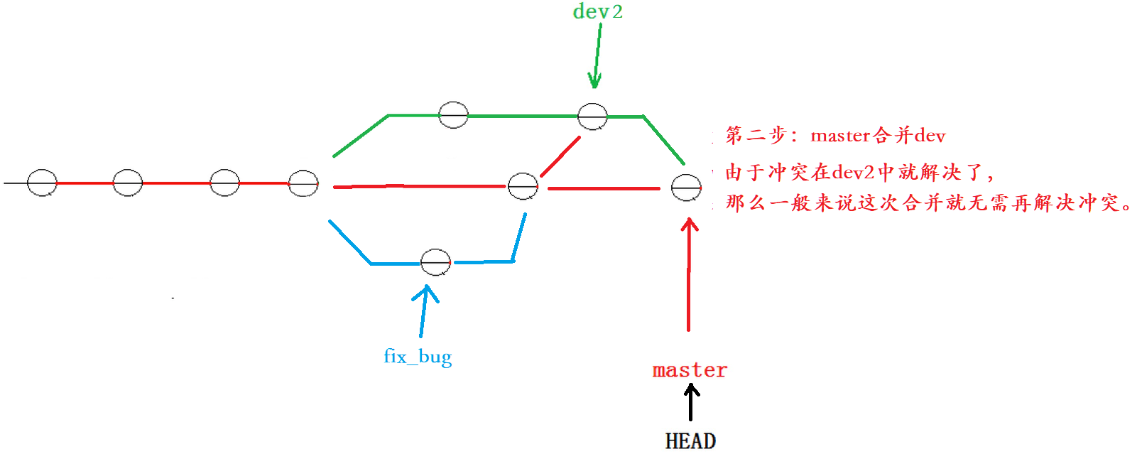
【Git原理和使用】Git 分支管理(创建、切换、合并、删除、bug分支)
一、理解分支 我们可以把分支理解为一个分身,这个分身是与我们的主身是相互独立的,比如我们的主身在这个月学C,而分身在这个月学java,在一个月以后我们让分身与主身融合,这样主身在一个月内既学会了C,也学…...

义乌购的反爬虫机制怎么应对?
在面对义乌购的反爬虫机制时,可以采取以下几种策略来应对: 1. 使用代理IP 义乌购可能会对频繁访问的IP地址进行限制,因此使用代理IP可以有效地隐藏爬虫的真实IP地址,避免被封禁。可以构建一个代理IP池,每次请求时随机…...

消息中间件面试
RabbitMQ 如何保证消息不丢失 消息重复消费 死信交换机 消息堆积怎么解决 高可用机制 Kafka 如何保证消息不丢失 如何保证消息的顺序性 高可用机制 数据清理机制 实现高性能的设计...

基于CLIP和DINOv2实现图像相似性方面的比较
概述 在人工智能领域,CLIP和DINOv2是计算机视觉领域的两大巨头。CLIP彻底改变了图像理解,而DINOv2为自监督学习带来了新的方法。 在本文中,我们将踏上一段旅程,揭示定义CLIP和DINOv2的优势和微妙之处。我们的目标是发现这些模型…...

利用Python爬虫获取API接口:探索数据的力量
引言 在当今数字化时代,数据已成为企业、研究机构和个人获取信息、洞察趋势和做出决策的重要资源。Python爬虫作为一种高效的数据采集工具,能够帮助我们自动化地从互联网上获取大量的数据。而API接口作为数据获取的重要途径之一,为我们提供了…...

【LeetCode】力扣刷题热题100道(1-5题)附源码 链表 子串 中位数 回文子串(C++)
目录 1.两数之和 2.两数相加-链表 3.无重复字符的最长子串 4.寻找两个正序数组的中位数 5.最长回文子串 1.两数之和 给定一个整数数组 nums 和一个整数目标值 target,请你在该数组中找出 和为目标值 target 的那 两个 整数,并返回它们的数组下标。…...

Docker启动失败 - 解决方案
Docker启动失败 - 解决方案 问题原因解决方案service问题 问题 重启docker失败: toolchainendurance:~$ sudo systemctl restart docker Job for docker.service failed because:the control process exited with error codesee:"systemctl status docker.se…...

【Duilib】 List控件支持多选和获取选择的多条数据
问题 使用Duilib库写的一个UI页面用到了List控件,功能变动想支持选择多行数据。 分析 1、List控件本身支持使用SetMultiSelect接口设置是否多选: void SetMultiSelect(bool bMultiSel);2、List控件本身支持使用GetNextSelItem接口获取选中的下一个索引…...

android系统的一键编译与非一键编译 拆包 刷机方法
1.从远程仓库下载源码 别人已经帮我下载好了在Ubuntu上。并给我权限:chmod -R ow /data/F200/F200-master/ 2.按照readme.txt步骤操作 安装编译环境: sudo apt-get update sudo apt-get install git-core gnupg flex bison gperf build-essential z…...

SQL语言的函数实现
SQL语言的函数实现 引言 随着大数据时代的到来,数据的存储和管理变得越来越复杂。SQL(结构化查询语言)作为关系数据库的标准语言,其重要性不言而喻。在SQL语言中,函数是一个重要的组成部分,可以有效地帮助…...

OSPF - 2、3类LSA(Network-LSA、NetWork-Sunmmary-LSA)
前篇博客有对常用LSA的总结 2类LSA(Network-LSA) DR产生泛洪范围为本区域 作用: 描述MA网络拓扑信息和网络信息,拓扑信息主要描述当前MA网络中伪节点连接着哪几台路由。网络信息描述当前网络的 掩码和DR接口IP地址。 影响邻居建立中说到…...

运动相机拍摄的视频打不开怎么办
3-10 GoPro和大疆DJI运动相机的特点,小巧、高清、续航长、拍摄稳定,很多人会在一些重要场合用来拍摄视频,比如可以用来拿在手里拍摄快速运动中的人等等。 但是毕竟是电子产品,有时候是会出点问题的,比如意外断电、摔重…...

SpringBoot | 使用Apache POI库读取Excel文件介绍
关注WX:CodingTechWork 介绍 在日常开发中,我们经常需要处理Excel文件中的数据。无论是从数据库导入数据、处理数据报表,还是批量生成数据,都可能会遇到需要读取和操作Excel文件的场景。本文将详细介绍如何使用Java中的Apache PO…...

从configure.ac到构建环境:解析Mellanox OFED内核模块构建脚本
在软件开发过程中,特别是在处理复杂的内核模块如Mellanox OFED(OpenFabrics Enterprise Distribution)时,构建一个可移植且高效的构建系统至关重要。Autoconf和Automake等工具在此过程中扮演着核心角色。本文将深入解析一个用于准备Mellanox OFED内核模块构建环境的Autocon…...

c#使用SevenZipSharp实现压缩文件和目录
封装了一个类,方便使用SevenZipSharp,支持加入进度显示事件。 双重加密压缩工具范例: using SevenZip; using System; using System.Collections.Generic; using System.IO; using System.Linq; using System.Text; using System.Threading.…...

长鑫存储逆袭:从近10年亏损超366亿到盈利超预期,能否成“中国海力士”?
长鑫存储逆袭:从巨亏到盈利超预期,能否成为“中国海力士”?“韩国巨头布局存储,中国巨头热衷于外卖。”这一波存储涨价潮,很多人用戏谑的方式来表达对中国几家互联网公司的“恨铁不成钢”。但长鑫存储却凭借一份极度亮…...

Real-ESRGAN终极指南:让模糊图像瞬间清晰的AI魔法
Real-ESRGAN终极指南:让模糊图像瞬间清晰的AI魔法 【免费下载链接】Real-ESRGAN Real-ESRGAN aims at developing Practical Algorithms for General Image/Video Restoration. 项目地址: https://gitcode.com/gh_mirrors/re/Real-ESRGAN 你是否曾经为那些模…...

突发!Karpathy 加入 Anthropic,重回一线搞研发
①就在刚刚不久,前 OpenAI 创始团队成员 Andrej Karpathy 发推宣布加入 Anthropic。我已加入 Anthropic。我认为未来几年大语言模型(LLM)领域的前沿发展将极具塑造性。我非常兴奋能加入这里的团队,重新投入研发工作。我对教育事业…...

AI 写的鸿蒙 ArkTS 代码能跑?我测了 37 个案例,翻车率 60%
先扔结论:如果你现在把 Claude 或 Cursor 当成 ArkTS 专家来用,大概率会掉坑里。我上周闲得慌,跑了 37 个常见开发场景的测试,结果 AI 生成的代码能直接编译通过的,不到四成。剩下的要么语法错误,要么用了废…...
)
软件工程师在智能体视觉时代的机遇(22)
重磅预告:本专栏将独家连载系列丛书《智能体视觉技术与应用》部分精华内容,该书是世界首套系统阐述“因式智能体”视觉理论与实践的专著,特邀美国 TypeOne 公司首席科学家、斯坦福大学博士 Bohan 担任技术顾问。Bohan先生师从美国三院院士、“…...

3分钟学会:如何用Chrome扩展一键保存完整网页内容
3分钟学会:如何用Chrome扩展一键保存完整网页内容 【免费下载链接】full-page-screen-capture-chrome-extension One-click full page screen captures in Google Chrome 项目地址: https://gitcode.com/gh_mirrors/fu/full-page-screen-capture-chrome-extension…...

用C语言搞定PTA数据结构7-1天梯地图:迪杰斯特拉算法实战与避坑指南
从零实现PTA天梯地图:双权重迪杰斯特拉算法全解析 当面对PTA数据结构7-1天梯地图这类双权重图的最短路径问题时,许多初学者会陷入算法选择的困境。本文将彻底拆解如何用C语言实现这一经典题目,不仅教你写出能AC的代码,更重要的是掌…...

【Redis | 第一篇】Redis常见命令
目录 一、Redis数据结构介绍 二、Redis的通用命令 三、String类型 3.1 key的层级结构 四、Hash类型 五、List类型 六、Set类型 一、Redis数据结构介绍 Redis是一个key-value的数据库,key一般是字符串类型,不过value的类型多种多样。 二、Redis的…...
)
为什么顶尖思想家团队只用Perplexity搜名言?——独家披露哈佛肯尼迪学院实测数据:准确率92.4%,响应延迟<1.7s(附配置白皮书)
更多请点击: https://kaifayun.com 第一章:为什么顶尖思想家团队只用Perplexity搜名言?——独家披露哈佛肯尼迪学院实测数据:准确率92.4%,响应延迟<1.7s(附配置白皮书) 在哈佛肯尼迪学院政…...
)
【物联网专业】案例9_2:控制数码管(定时器中断)
文章目录0 文章介绍1 仿真图2 效果图3 不完整代码4 思考题0 文章介绍 对应定时器/计数器案例目标的实现 用计数器中断0(P3^4)控制数码管段选 P1^6)控制数码位选 1 仿真图 2 效果图 3 不完整代码 复制该代码,其中有7个补充点&#…...