Yolov5-Face 原理解析及算法解析
YOLOv5-Face
文章目录
- YOLOv5-Face
- 1. 为什么人脸检测 = 一般检测?
- 1.1 YOLOv5Face人脸检测
- 1.2 YOLOv5Face Landmark
- 2.YOLOv5Face的设计目标和主要贡献
- 2.1 设计目标
- 2.2 主要贡献
- 3. YOLOv5Face架构
- 3.1 模型架构
- 3.1.1 模型示意图
- 3.1.2 CBS模块
- 3.1.3 Head输出
- 3.1.4 stem结构
- 3.1.5 CSP结构
- 3.1.9 SPP结构
- 3.2 输入端的改进
- 3.3 Landmark回归
- 3.3.1 输出 Landmark
- 3.3.2 Landmark损失函数Wing
- 3.3.3 Wing Loss
- 3.4 后处理NMS
- 3.4.1 yolov5
- 3.4.2 yolov5s-face
- 4.模型训练
- 4.1 下载源码
- 4.2 下载widerface数据集
- 4.3 运行train2yolo.py和val2yolo.py
- 4.4 train
- 4.4.1 更改训练配置文件
- 4.4.2 训练可视化
- 4.4.3 相关报错
- 4.5 detect
- 4.6 ONNX导出及TensorRT环境配置
- 4.7 OnnXruntime推理
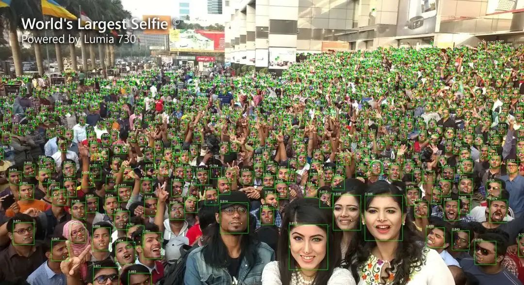
近年来,CNN在人脸检测方面已经得到广泛的应用。但是许多人脸检测器都是需要使用特别设计的人脸检测器来进行人脸的检测,而YOLOv5的作者则是把人脸检测作为一个一般的目标检测任务来看待的。
YOLOv5Face在YOLOv5的基础上添加了一个 5-Point Landmark Regression Head(关键点回归),并对Landmark Regression Head使用了Wing loss进行约束。YOLOv5Face设计了不同模型尺寸的检测器,从大模型到超小模型,以实现在嵌入式或移动设备上的实时检测。
在WiderFace数据集上的实验结果表明,YOLOv5Face在几乎所有的Easy、Medium和Hard子集上都能达到最先进的性能,超过了特定设计的人脸检测器。
Github地址:https://www.github.com/deepcam-cn/yolov5-face
1. 为什么人脸检测 = 一般检测?
1.1 YOLOv5Face人脸检测
在YOLOv5Face的方法中是把人脸检测作为一个一般的目标检测任务。与TinaFace想法类似把人脸作为一个目标。正如在TinaFace中所讨论的:
- 从数据的角度来看,人脸所具有的诸如姿态、尺度、遮挡、光照以及模糊等也会出现在其他的一般检测任务之中;
- 从面部的独特属来看性,如表情和化妆,也可以对应一般检测问题中的形状变化和颜色变化。
1.2 YOLOv5Face Landmark
Landmark相对来说是一个特殊的存在,但他们也并不是唯一的。它们只是一个物体的关键点。例如,在车牌检测中,也使用了Landmark。在目标预测模型的Head中添加Landmark回归相对来说是一键简单的事情。那么从人脸检测所面临的挑战来看,多尺度、小人脸、密集场景等在一般的目标检测中都存在。因此,人脸检测完全可以看作一个一般目标检测子任务。
2.YOLOv5Face的设计目标和主要贡献
2.1 设计目标
YOLOv5Face针对人脸检测的对YOLOv5进行了再设计和修改,考虑到大人脸、小人脸、Landmark监督等不同的复杂性和应用。YOLOv5Face的目标是为不同的应用程序提供一个模型组合,从非常复杂的应用程序到非常简单的应用程序,以在嵌入式或移动设备上获得性能和速度的最佳权衡。
2.2 主要贡献
- 重新设计了YOLOV5来作为一个人脸检测器,并称之为YOLOv5Face。对网络进行了关键的修改,以提高平均平均精度(mAP)和速度方面的性能;
- 设计了一系列不同规模的模型,从大型模型到中型模型,再到超小模型,以满足不同应用中的需要。除了在YOLOv5中使用的Backbone外,还实现了一个基于ShuffleNetV2的Backbone,它为移动设备提供了最先进的性能和快速的速度;
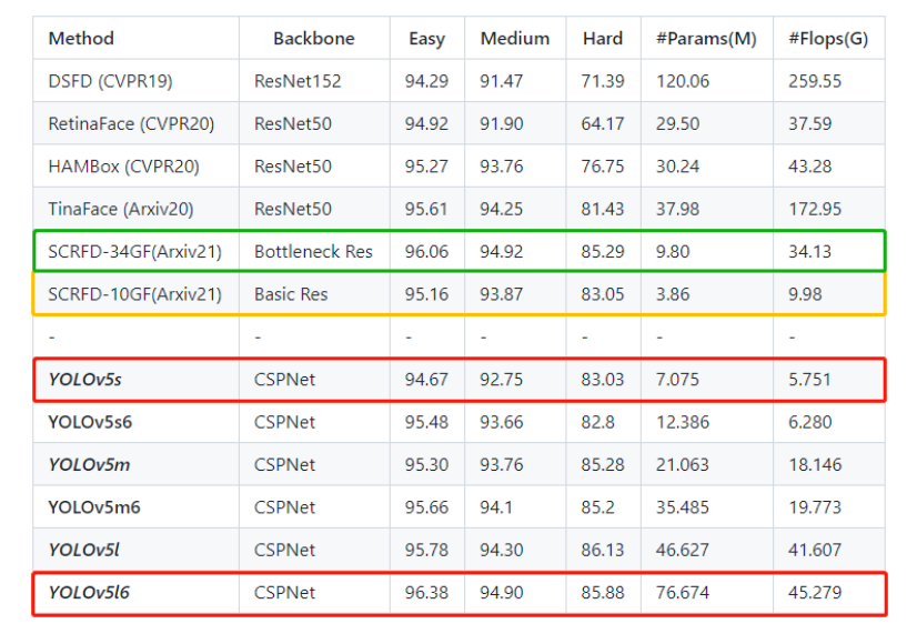
- 在WiderFace数据集上评估了YOLOv5Face模型。在VGA分辨率的图像上,几乎所有的模型都达到了SOTA性能和速度。这也证明了前面的结论,不需要重新设计一个人脸检测器,因为YOLO5就可以完成它。
3. YOLOv5Face架构
3.1 模型架构
3.1.1 模型示意图
YOLOv5Face是以YOLOv5作为Baseline来进行改进和再设计以适应人脸检测。这里主要是检测小脸和大脸的修改。
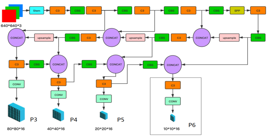
YOLO5人脸检测器的网络架构如图1所示。它由Backbone、Neck和Head组成,描述了整体的网络体系结构。在YOLOv5中,使用了CSPNet Backbone。在Neck中使用了SPP和PAN来融合这些特征。在Head中也都使用了回归和分类。
3.1.2 CBS模块
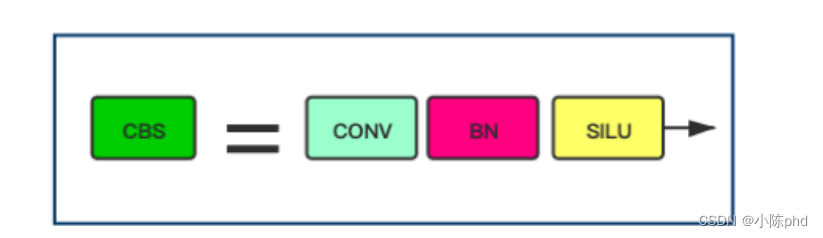
在图中,定义了一个CBS Block,它由Conv、BN和SiLU激活函数组成。CBS Block也被用于许多其他Block之中。
class Conv(nn.Module):# Standard convolutiondef __init__(self, c1, c2, k=1, s=1, p=None, g=1, act=True): # ch_in, ch_out, kernel, stride, padding, groupssuper(Conv, self).__init__()# 卷积层self.conv = nn.Conv2d(c1, c2, k, s, autopad(k, p), groups=g, bias=False)# BN层self.bn = nn.BatchNorm2d(c2)# SiLU激活层self.act = nn.SiLU() if act is True else (act if isinstance(act, nn.Module) else nn.Identity())def forward(self, x):return self.act(self.bn(self.conv(x)))
3.1.3 Head输出
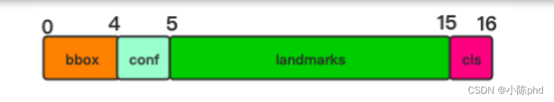
显示Head的输出标签,其中包括边界框(bbox)、置信度(conf)、分类(cls)和5-Point Landmarks。这些Landmarks是对YOLOv5的改进点,使其成为一个具有Landmarks输出的人脸检测器。如果没有Landmarks,最后一个向量的长度应该是6而不是16。框(4)+置信度(1)+关键点(5*2)+cls(类别)
P3中的输出尺寸80×80×16,P4中的40×40×16,P5中的20×20×16,可选P6中的10×10×16为每个Anchor。实际的尺寸应该乘以Anchor的数量。
3.1.4 stem结构
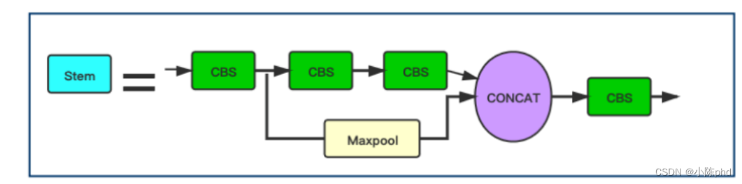
图为stem结构,它用于取代YOLOv5中原来的Focus层。在YOLOv5中引入Stem块用于人脸检测是YOLOv5Face的创新之一。
class StemBlock(nn.Module):def __init__(self, c1, c2, k=3, s=2, p=None, g=1, act=True):super(StemBlock, self).__init__()# 3×3卷积self.stem_1 = Conv(c1, c2, k, s, p, g, act)# 1×1卷积self.stem_2a = Conv(c2, c2 // 2, 1, 1, 0)# 3×3卷积self.stem_2b = Conv(c2 // 2, c2, 3, 2, 1)# 最大池化层self.stem_2p = nn.MaxPool2d(kernel_size=2, stride=2, ceil_mode=True)# 1×1卷积self.stem_3 = Conv(c2 * 2, c2, 1, 1, 0)def forward(self, x):stem_1_out = self.stem_1(x)stem_2a_out = self.stem_2a(stem_1_out)stem_2b_out = self.stem_2b(stem_2a_out)stem_2p_out = self.stem_2p(stem_1_out)out = self.stem_3(torch.cat((stem_2b_out, stem_2p_out), 1))return out
用Stem模块替代网络中原有的Focus模块,提高了网络的泛化能力,降低了计算复杂度,同时性能也没有下降。Stem模块的图示中虽然都是用的CBS,但是看代码可以看出来第2个和第4个CBS是1×1卷积,第1个和第3个CBS是3×3,stride=2的卷积。配合yaml文件可以看到stem以后图像大小由640×640变成了160×160。
3.1.5 CSP结构
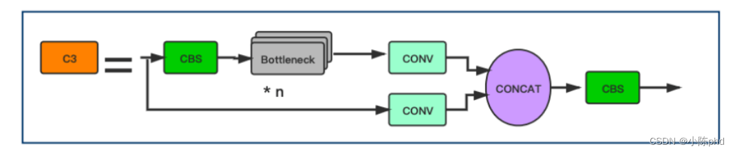
CSP Block的设计灵感来自于DenseNet。但是,不是在一些CNN层之后添加完整的输入和输出,输入被分成 2 部分。其中一半通过一个CBS Block,即一些Bottleneck Blocks,另一半是经过Conv层进行计算:
class C3(nn.Module):# CSP Bottleneck with 3 convolutionsdef __init__(self, c1, c2, n=1, shortcut=True, g=1, e=0.5): # ch_in, ch_out, number, shortcut, groups, expansionsuper(C3, self).__init__()c_ = int(c2 * e) # hidden channelsself.cv1 = Conv(c1, c_, 1, 1)self.cv2 = Conv(c1, c_, 1, 1)self.cv3 = Conv(2 * c_, c2, 1) # act=FReLU(c2)self.m = nn.Sequential(*[Bottleneck(c_, c_, shortcut, g, e=1.0) for _ in range(n)])def forward(self, x):return self.cv3(torch.cat((self.m(self.cv1(x)), self.cv2(x)), dim=1))
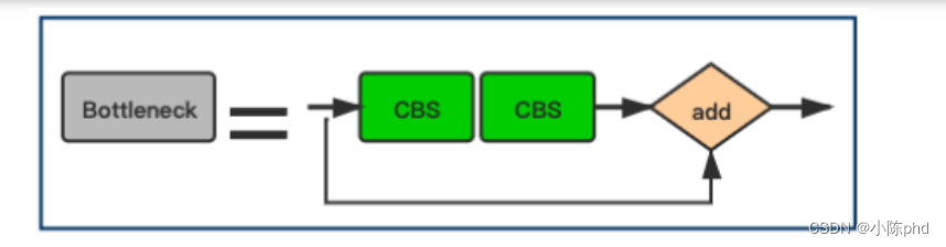
其中Bottleneck层表示为:
class Bottleneck(nn.Module):# Standard bottleneckdef __init__(self, c1, c2, shortcut=True, g=1, e=0.5): # ch_in, ch_out, shortcut, groups, expansionsuper(Bottleneck, self).__init__()c_ = int(c2 * e) # hidden channels#第1个CBS模块self.cv1 = Conv(c1, c_, 1, 1)#第2个CBS模块self.cv2 = Conv(c_, c2, 3, 1, g=g)#元素add操作self.add = shortcut and c1 == c2def forward(self, x):return x + self.cv2(self.cv1(x)) if self.add else self.cv2(self.cv1(x))
3.1.9 SPP结构
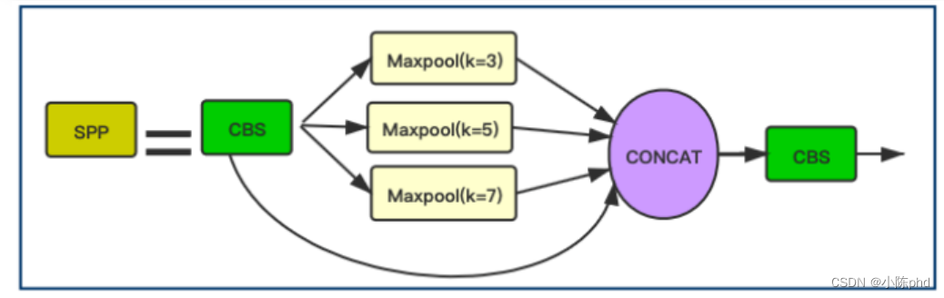
YOLOv5Face在这个Block中把YOLOv5中的13×13,9×9,5×5的kernel size被修改为7×7,5×5,3×3,这个改进更适用于人脸检测并提高了人脸检测的精度。
class SPP(nn.Module):# 这里主要是讲YOLOv5中的kernel=(5,7,13)修改为(3, 5, 7)def __init__(self, c1, c2, k=(3, 5, 7)):super(SPP, self).__init__()c_ = c1 // 2 # hidden channels# 对应第1个CBS Blockself.conv1 = Conv(c1, c_, 1, 1)# 对应第2个 cat后的 CBS Blockself.conv2 = Conv(c_ * (len(k) + 1), c2, 1, 1)# ModuleList=[3×3 MaxPool2d,5×5 MaxPool2d,7×7 MaxPool2d]self.m = nn.ModuleList([nn.MaxPool2d(kernel_size=x, stride=1, padding=x // 2) for x in k])def forward(self, x):x = self.conv1(x)return self.conv2(torch.cat([x] + [m(x) for m in self.m], 1))
同时,YOLOv5Face添加一个stride=64的P6输出块,P6可以提高对大人脸的检测性能。(之前的人脸检测模型大多关注提高小人脸的检测性能,这里作者关注了大人脸的检测效果,提高大人脸的检测性能来提升模型整体的检测性能)。P6的特征图大小为10x10。
注意,这里只考虑VGA分辨率的输入图像。为了更精确地说,输入图像的较长的边缘被缩放到640,并且较短的边缘被相应地缩放。较短的边缘也被调整为SPP块最大步幅的倍数。例如,当不使用P6时,较短的边需要是32的倍数;当使用P6时,较短的边需要是64的倍数。
3.2 输入端的改进
一些目标检测的数据增广方法并不适合用在人脸检测中,包括上下翻转和Mosaic数据增广。
- 删除上下翻转可以提高模型性能。
- 对小人脸进行Mosaic数据增广反而会降低模型性能,但是对中尺度和大尺度人脸进行Mosaic可以提高性能。
- 随机裁剪有助于提高性能。
备注:COCO数据集和WiderFace数据集尺度有差异,WiderFace数据集小尺度数据相对较多。
3.3 Landmark回归
3.3.1 输出 Landmark
Landmark是人脸的重要特征。它们可以用于人脸比对、人脸识别、面部表情分析、年龄分析等任务。传统Landmark由68个点组成。它们被简化为5点时,这5点Landmark就被广泛应用于面部识别。人脸标识的质量直接影响人脸对齐和人脸识别的质量。
- 一般的物体检测器不包括Landmark。可以直接将其添加为回归Head。因此,作者将它添加到YOLO5Face中。Landmark输出将用于对齐人脸图像,然后将其发送到人脸识别网络。
3.3.2 Landmark损失函数Wing
用于Landmark回归的一般损失函数为L2、L1或smooth-L1。MTCNN使用的就是L2损失函数。然而,作者发现这些损失函数对小的误差并不敏感。为了克服这个问题,提出了Wing loss:
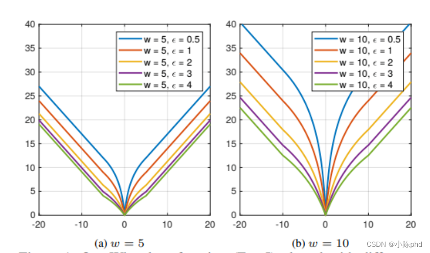
wing ( x ) = { w ln ( 1 + ∣ x ∣ / ϵ ) if ∣ x ∣ < w ∣ x ∣ − C otherwise \operatorname{wing}(x)= \begin{cases}w \ln (1+|x| / \epsilon) & \text { if }|x|<w \\ |x|-C & \text { otherwise }\end{cases} wing(x)={wln(1+∣x∣/ϵ)∣x∣−C if ∣x∣<w otherwise
w : w: w: 正数 w w w 将非线性部分的范围限制在 [ − w , w ] [-w, w] [−w,w] 区间内;
ϵ \epsilon ϵ :约束非线性区域的曲率,并且 C = w − w ln ( 1 + x ϵ ) C=w-w \ln \left(1+\frac{x}{\epsilon}\right) C=w−wln(1+ϵx) 是一个常数,可与平滑的来连接分段 的线性和非线性部分。 ϵ \epsilon ϵ 的取值是一个很小的数值,因为它会使网络训练变得不稳定,并且会 因为很小的误差导致梯度爆炸问题。
实际上,的Wing loss函数的非线性部分只是简单地采用 ln ( x ) \ln (x) ln(x) 在 [ ϵ / w , 1 + ϵ / w ] [\epsilon / w, 1+\epsilon / w] [ϵ/w,1+ϵ/w] 之间的曲 线,并沿X轴和 Y Y Y 轴将其缩放比例为W。另外,沿 Y Y Y 轴应用平移以使wing ( 0 ) = 0 (0)=0 (0)=0, 并在损失函 数上施加连续性。
Landmark点向量 s = { s i } s=\left\{s_i\right\} s={si} 与其ground truth s ′ = { s i } s^{\prime}=\left\{s_i\right\} s′={si} 的损失函数为:
loss L ( s ) = ∑ i wing ( s i − s i ′ ) \operatorname{loss}_L(s)=\sum_i \operatorname{wing}\left(s_i-s_i^{\prime}\right) lossL(s)=i∑wing(si−si′)
其中 i = 1 , 2 , … , 10 i=1,2, \ldots, 10 i=1,2,…,10 。
设YOLOv5中通用的目标检测损失函数为 l o s s O l o s s_O lossO ,则新的总损失函数为:
loss ( s ) = loss O + λ L ⋅ loss L \operatorname{loss}(s)=\operatorname{loss}_O+\lambda_L \cdot \operatorname{loss}_L loss(s)=lossO+λL⋅lossL
其中 λ L \lambda_L λL 为Landmark回归损失函数的权重因子。
landmark的获取:其中 i = 1 , 2 , … , 10 i=1,2, \ldots, 10 i=1,2,…,10 。
设YOLOv5 中通用的目标检测损失函数为 l o s s O l o s s_O lossO ,则新的总损失函数为:
loss ( s ) = loss O + λ L ⋅ loss L \operatorname{loss}(s)=\operatorname{loss}_O+\lambda_L \cdot \operatorname{loss}_L loss(s)=lossO+λL⋅lossL
其中 λ L \lambda_L λL 为Landmark回归损失函数的权重因子。
landmark的获取:
#landmarks
lks = t[:,6:14]
lks_mask = torch.where(lks < 0, torch.full_like(lks, 0.), torch.full_like(lks, 1.0))
#应该是关键点的坐标除以anch的宽高才对,便于模型学习。使用gwh会导致不同关键点的编码不同,没有统一的参考标准
lks[:, [0, 1]] = (lks[:, [0, 1]] - gij)
lks[:, [2, 3]] = (lks[:, [2, 3]] - gij)
lks[:, [4, 5]] = (lks[:, [4, 5]] - gij)
lks[:, [6, 7]] = (lks[:, [6, 7]] - gij)
Wing Loss的计算如下:
class WingLoss(nn.Module):def __init__(self, w=10, e=2):super(WingLoss, self).__init__()# https://arxiv.org/pdf/1711.06753v4.pdf Figure 5self.w = wself.e = eself.C = self.w - self.w * np.log(1 + self.w / self.e)def forward(self, x, t, sigma=1): #这里的x,t分别对应之后的pret,truelweight = torch.ones_like(t) #返回一个大小为1的张量,大小与t相同weight[torch.where(t==-1)] = 0diff = weight * (x - t)abs_diff = diff.abs()flag = (abs_diff.data < self.w).float()y = flag * self.w * torch.log(1 + abs_diff / self.e) + (1 - flag) * (abs_diff - self.C) #全是0,1return y.sum()class LandmarksLoss(nn.Module):# BCEwithLogitLoss() with reduced missing label effects.def __init__(self, alpha=1.0):super(LandmarksLoss, self).__init__()self.loss_fcn = WingLoss()#nn.SmoothL1Loss(reduction='sum')self.alpha = alphadef forward(self, pred, truel, mask): #预测的,真实的 600(原来为62*10)(推测是去掉了那些没有标注的值)loss = self.loss_fcn(pred*mask, truel*mask) #一个值(tensor)return loss / (torch.sum(mask) + 10e-14)
分析比较L1,L2和Smooth L1损失函数
loss ( s , s ′ ) = ∑ i = 1 2 L f ( s i − s i ′ ) \operatorname{loss}\left(\mathbf{s}, \mathbf{s}^{\prime}\right)=\sum_{i=1}^{2 L} f\left(s_i-s_i^{\prime}\right) loss(s,s′)=i=1∑2Lf(si−si′)
其中 s s s 是人脸关键点的ground-truth,函数 f ( x ) f(x) f(x) 就等价于:
L1 loss
L 1 ( x ) = ∣ x ∣ L 1(x)=|x| L1(x)=∣x∣
L2 loss
L 2 ( x ) = 1 2 x 2 L 2(x)=\frac{1}{2} x^2 L2(x)=21x2
Smooth L 1 ( x ) : smooth L 1 ( x ) = { 1 2 x 2 if ∣ x ∣ < 1 ∣ x ∣ − 1 2 otherwise \operatorname{Smooth}_{L 1}(x): \operatorname{smooth}_{L 1}(x)= \begin{cases}\frac{1}{2} x^2 & \text { if }|x|<1 \\ |x|-\frac{1}{2} & \text { otherwise }\end{cases} SmoothL1(x):smoothL1(x)={21x2∣x∣−21 if ∣x∣<1 otherwise
损失函数对 x x x 的导数分别为:
d L 2 ( x ) d x = x \frac{d L_2(x)}{d x}=x dxdL2(x)=x
d L 1 ( x ) d x = { 1 if x ≥ 0 − 1 otherwise \frac{d L_1(x)}{d x}= \begin{cases}1 & \text { if } x \geq 0 \\ -1 & \text { otherwise }\end{cases} dxdL1(x)={1−1 if x≥0 otherwise
d smooth L 1 ( x ) d x = { x if ∣ x ∣ < 1 ± 1 otherwise \frac{d \operatorname{smooth}_{L 1}(x)}{d x}= \begin{cases}x & \text { if }|x|<1 \\ \pm 1 & \text { otherwise }\end{cases} dxdsmoothL1(x)={x±1 if ∣x∣<1 otherwise
-
L2损失函数,当 x x x 增大时L2 loss对 x x x 的导数也增大,这就导致训练初期,预测值与groundtruth差异过大时,损失函数对预测值的梯度十分大,导致训练不稳定。
-
L1 loss的导数为常数,在训练后期,预测值与ground-truth差异很小时,损失对预测值的导 数的绝对值仍然为 1 ,此时学习率(learning rate)如果不变,损失函数将在稳定值附近波动, 难以继续收敛达到更高精度。
-
smooth L1损失函数,在x较小时,对 x x x 的梯度也会变小,而在 x x x 很大时,对 x x x 的梯度的绝对值 达到上限 1,也不会太大以至于破坏网络参数。smooth L1完美地避开了L1和L2损失的缺 陷。
此外,根据fast rcnn的说法, “… L1 loss that is less sensitive to outliers than the L2 loss used in R-CNN and SPPnet.” 也就是smooth L1让loss对于离群点更加鲁棒,即相比于L2 损失函数,其对离群点、异常值 (outlier) 不敏感,梯度变化相对更小,训练时不容易跑飞。
上图描绘了这些损失函数的曲线图。需要注意的是,Smoolth L1损失是Huber损失的一种特殊情况,L2损失函数在人脸关键点检测中被广泛应用,然而,L2损失对异常值很敏感。
3.3.3 Wing Loss
所有损失函数在出现较大误差时表现良好。这说明神经网络的训练应更多地关注具有小或中误差的样本。为了实现此目标,提出了一种新的损失函数,即基于CNN的面部Landmark定位的Wing Loss。

当NME在0.04的时候,测试数据比例已经接近1了,所以在0.04到0.05这一段,也就是所谓的large errros段,并没有分布更多的数据,说明各损失函数在large errors段都表现很好。
模型表现不一致的地方就在于small errors和medium errors段,例如,在NME为0.02的地方画一根竖线,相差甚远的。因此作者提出训练过程中应该更多关注samll or medium range errros样本。
可以使用 ln x \ln x lnx 来增强小误差的影响,它的梯度是 1 x \frac{1}{x} x1, 对于接近0的值就会越大,optimal step size 为 x 2 x^2 x2 ,这样gradient就由small errors “主导", step size由large errors “主导"。这样可 以恢复不同大小误差之间的平衡。但是,为了防止在可能的错误方向上进行较大的更新步骤,重要的是不要过度补偿较小的定位 错误的影响。这可以通过选择具有正偏移量的对数函数来实现。
但是这种类型的损失函数适用于处理相对较小的定位误差。在wild人脸关键点检测中,可能会 处理极端姿势,这些姿势最初的定位误差可能非常大,在这种情况下,损失函数应促进从这些 大错误中快速恢复。这表明损失函数的行为应更像 L 1 L 1 L1 或 L 2 L 2 L2 。由于 L 2 L 2 L2 对异常值敏感,因此选择 了L1。
所以,Wing Loss对于小误差,它应该表现为具有偏移量的对数函数,而对于大误差,则应表现为 L 1 L 1 L1 。
3.4 后处理NMS
3.4.1 yolov5
def non_max_suppression(prediction, conf_thres=0.25, iou_thres=0.45, classes=None, agnostic=False, labels=()):"""Performs Non-Maximum Suppression (NMS) on inference resultsReturns:detections with shape: nx6 (x1, y1, x2, y2, conf, cls)"""nc = prediction.shape[2] -5 # number of classes
3.4.2 yolov5s-face
def non_max_suppression_face(prediction, conf_thres=0.25, iou_thres=0.45, classes=None, agnostic=False, labels=()):"""Performs Non-Maximum Suppression (NMS) on inference resultsReturns:detections with shape: nx6 (x1, y1, x2, y2, conf, cls)"""# 不同之处nc = prediction.shape[2] - 15 # number of classes
4.模型训练
4.1 下载源码
git clone https://github.com/deepcam-cn/yolov5-face
4.2 下载widerface数据集
下载后,解压缩位置放到yolov5-face-master项目里data文件夹下的widerface文件夹下。
https://drive.google.com/file/d/1tU_IjyOwGQfGNUvZGwWWM4SwxKp2PUQ8/view?usp=sharing
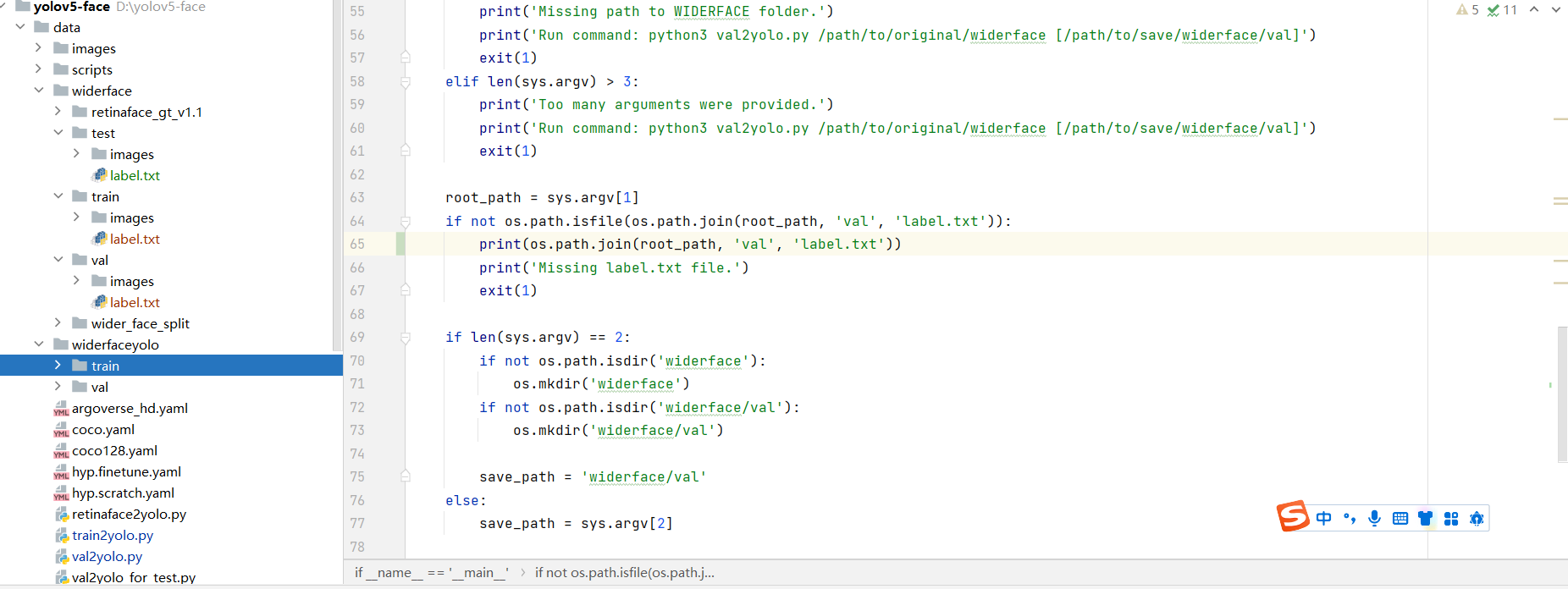
4.3 运行train2yolo.py和val2yolo.py
data文件夹下新建widerfaceyolo文件夹,子目录设立为train、test、val
python train2yolo.py ./widerface/train ../data/widerfaceyolo/train
python val2yolo.py ./widerface ../data/widerfaceyolo/val
把数据集转成yolo训练用的格式。完成后文件夹显示如下:

4.4 train
4.4.1 更改训练配置文件
widerface.yaml 更改目录为数据集目录
# train and val data as 1) directory: path/images/, 2) file: path/images.txt, or 3) list: [path1/images/, path2/images/]
train: ./data/widerfaceyolo/train  # 16551 images
val: ./data/widerfaceyolo/val  # 16551 images
#val: /ssd_1t/derron/yolov5-face/data/widerface/train/  # 4952 images# number of classes
nc: 1# class names
names: [ 'face']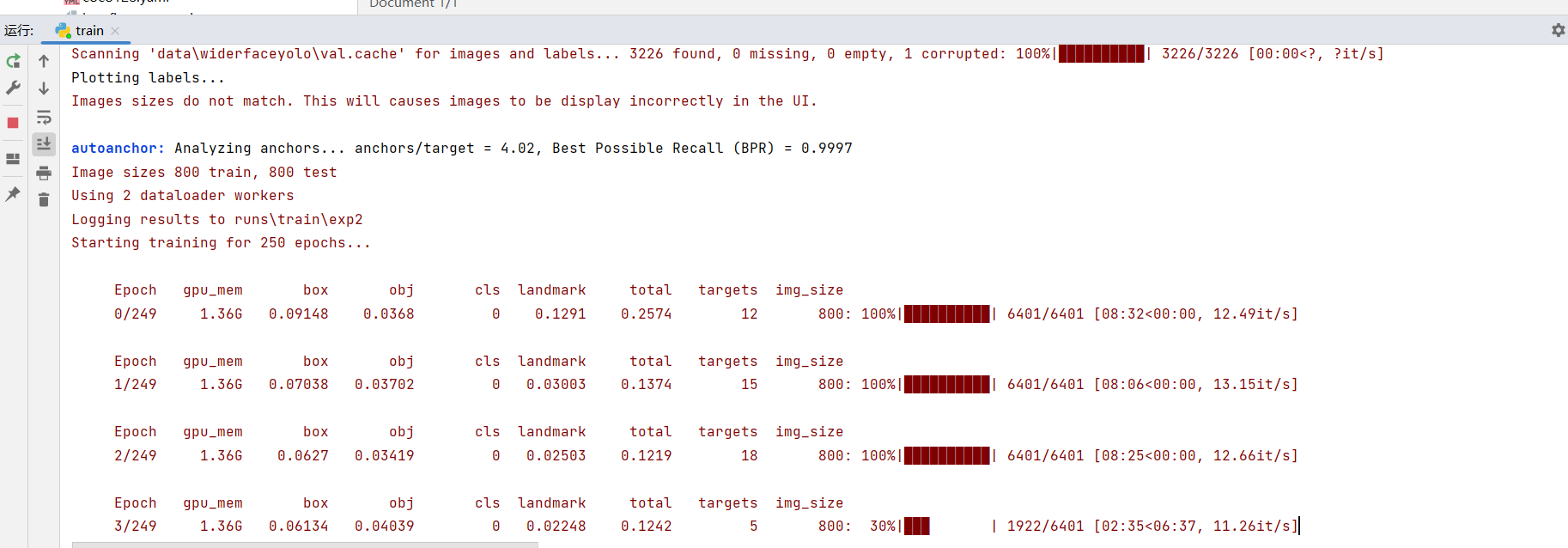
4.4.2 训练可视化
tensorboard --logdir runs/train
4.4.3 相关报错
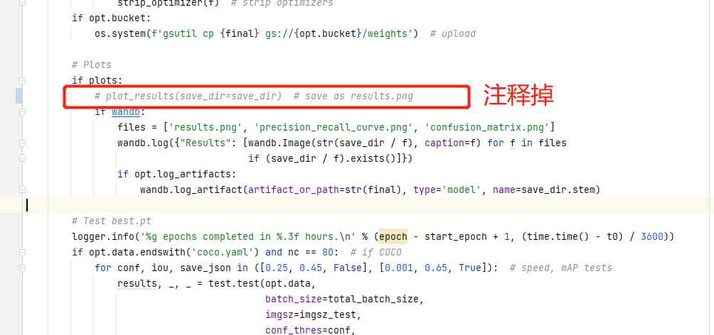
- 无法绘制图像
Traceback (most recent call last):File "D:\yolov5-face\train.py", line 523, in <module>train(hyp, opt, device, tb_writer, wandb)File "D:\yolov5-face\train.py", line 410, in trainplot_results(save_dir=save_dir) # save as results.pngFile "D:\yolov5-face\utils\plots.py", line 393, in plot_resultsassert len(files), 'No results.txt files found in %s, nothing to plot.' % os.path.abspath(save_dir)解决方案注释掉这行代码:
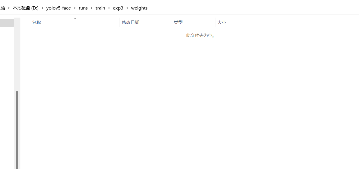
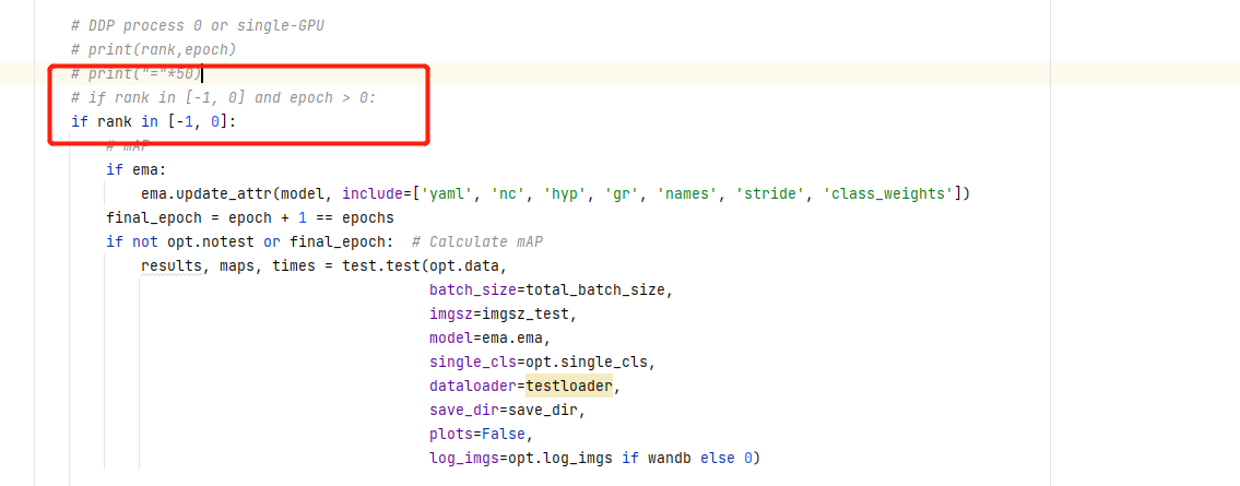
- 不保存权重
训练半天最后竟然发现保存权重为空,注释相关epoch大于20才保存权重代码
4.5 detect
更改代码
if __name__ == '__main__':parser = argparse.ArgumentParser()# 更改权重,指定权重类型parser.add_argument('--weights', nargs='+', type=str, default='yolov5s-face.pt', help='model.pt path(s)')parser.add_argument('--source', type=str, default='0', help='source') # file/folder, 0 for webcamparser.add_argument('--img-size', type=int, default=640, help='inference size (pixels)')parser.add_argument('--project', default=ROOT / 'runs/detect', help='save results to project/name')parser.add_argument('--name', default='exp', help='save results to project/name')parser.add_argument('--exist-ok', action='store_true', help='existing project/name ok, do not increment')parser.add_argument('--save-img', action='store_true', help='save results')parser.add_argument('--view-img', default=True,action='store_true', help='show results')opt = parser.parse_args()device = torch.device("cuda" if torch.cuda.is_available() else "cpu")model = load_model(opt.weights, device)detect(model, opt.source, device, opt.project, opt.name, opt.exist_ok, opt.save_img, opt.view_img)
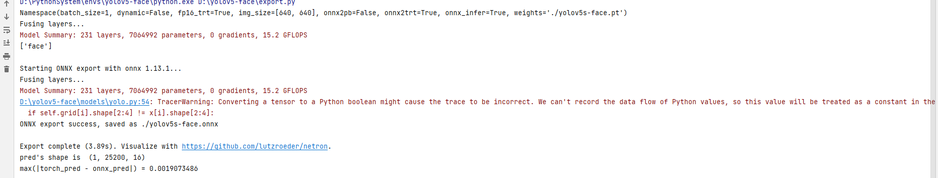
4.6 ONNX导出及TensorRT环境配置
"""Exports a YOLOv5 *.pt model to ONNX and TorchScript formatsUsage:$ export PYTHONPATH="$PWD" && python models/export.py --weights ./weights/yolov5s.pt --img 640 --batch 1
"""import argparse
import sys
import timesys.path.append('./')  # to run '$ python *.py' files in subdirectoriesimport torch
import torch.nn as nnimport models
from models.experimental import attempt_load
from utils.activations import Hardswish, SiLU
from utils.general import set_logging, check_img_size
import onnxif __name__ == '__main__':parser = argparse.ArgumentParser()parser.add_argument('--weights', type=str, default='./yolov5s-face.pt', help='weights path')  # from yolov5/models/parser.add_argument('--img_size', nargs='+', type=int, default=[640, 640], help='image size')  # height, widthparser.add_argument('--batch_size', type=int, default=1, help='batch size')parser.add_argument('--dynamic', action='store_true', default=False, help='enable dynamic axis in onnx model')parser.add_argument('--onnx2pb', action='store_true', default=False, help='export onnx to pb')parser.add_argument('--onnx_infer', action='store_true', default=True, help='onnx infer test')#=======================TensorRT=================================parser.add_argument('--onnx2trt', action='store_true', default=True, help='export onnx to tensorrt')parser.add_argument('--fp16_trt', action='store_true', default=True, help='fp16 infer')#================================================================opt = parser.parse_args()opt.img_size *= 2 if len(opt.img_size) == 1 else 1  # expandprint(opt)set_logging()t = time.time()# Load PyTorch modelmodel = attempt_load(opt.weights, map_location=torch.device('cpu'))  # load FP32 modeldelattr(model.model[-1], 'anchor_grid')model.model[-1].anchor_grid=[torch.zeros(1)] * 3 # nl=3 number of detection layersmodel.model[-1].export_cat = Truemodel.eval()labels = model.namesprint(labels)# exit()# Checksgs = int(max(model.stride))  # grid size (max stride)opt.img_size = [check_img_size(x, gs) for x in opt.img_size]  # verify img_size are gs-multiples# Input 给定一个输入img = torch.zeros(opt.batch_size, 3, *opt.img_size)  # image size(1,3,320,192) iDetection# Update modelfor k, m in model.named_modules():m._non_persistent_buffers_set = set()  # pytorch 1.6.0 compatibilityif isinstance(m, models.common.Conv):  # assign export-friendly activationsif isinstance(m.act, nn.Hardswish):m.act = Hardswish()elif isinstance(m.act, nn.SiLU):m.act = SiLU()# elif isinstance(m, models.yolo.Detect):#     m.forward = m.forward_export  # assign forward (optional)if isinstance(m, models.common.ShuffleV2Block):#shufflenet block nn.SiLUfor i in range(len(m.branch1)):if isinstance(m.branch1[i], nn.SiLU):m.branch1[i] = SiLU()for i in range(len(m.branch2)):if isinstance(m.branch2[i], nn.SiLU):m.branch2[i] = SiLU()y = model(img)  # dry run# ONNX exportprint('\nStarting ONNX export with onnx %s...' % onnx.__version__)f = opt.weights.replace('.pt', '.onnx')  # filenamemodel.fuse()  # only for ONNXinput_names=['input']output_names=['output']torch.onnx.export(model, img, f, verbose=False, opset_version=12, input_names=input_names,output_names=output_names,dynamic_axes = {'input': {0: 'batch'},'output': {0: 'batch'}} if opt.dynamic else None)# Checksonnx_model = onnx.load(f)  # load onnx modelonnx.checker.check_model(onnx_model)  # check onnx modelprint('ONNX export success, saved as %s' % f)# Finishprint('\nExport complete (%.2fs). Visualize with https://github.com/lutzroeder/netron.' % (time.time() - t))# exit()# onnx inferif opt.onnx_infer:import onnxruntimeimport numpy as npproviders =  ['CPUExecutionProvider']session = onnxruntime.InferenceSession(f, providers=providers)im = img.cpu().numpy().astype(np.float32) # torch to numpyy_onnx = session.run([session.get_outputs()[0].name], {session.get_inputs()[0].name: im})[0]print("pred's shape is ",y_onnx.shape)print("max(|torch_pred - onnx_pred|) =",abs(y.cpu().numpy()-y_onnx).max())
4.7 OnnXruntime推理
代码如下:
#!/usr/bin/env python
# -*- coding: utf-8 -*-
# @Time    : 2023/5/30 23:24
# @Author  : 陈伟峰
# @Site    :
# @File    : onnxruntime_infer.py
# @Software: PyCharm
import time
import numpy as np
import argparse
import onnxruntime
import os, torch
import cv2, copyfrom detect_face import scale_coords_landmarks, show_results
from utils.general import non_max_suppression_face, scale_coordsdef allFilePath(rootPath, allFIleList):  # 遍历文件fileList = os.listdir(rootPath)for temp in fileList:if os.path.isfile(os.path.join(rootPath, temp)):allFIleList.append(os.path.join(rootPath, temp))else:allFilePath(os.path.join(rootPath, temp), allFIleList)def my_letter_box(img, size=(640, 640)):  #'''将输入的图像img按照指定的大小size进行缩放和填充,使其适应指定的大小。具体来说,它首先获取输入图像的高度h、宽度w和通道数c,然后计算出缩放比例r,并根据缩放比例计算出新的高度new_h和宽度new_w。接着,它计算出在新图像中上、下、左、右需要填充的像素数,并使用cv2.resize函数将输入图像缩放到新的大小。最后,它使用cv2.copyMakeBorder函数在新图像的上、下、左、右四个方向进行填充,并返回填充后的图像img、缩放比例r、左侧填充像素数left和上方填充像素数topArgs:img:size:Returns:'''h, w, c = img.shape# cv2.imshow("res",img)# cv2.waitKey(0)r = min(size[0] / h, size[1] / w)new_h, new_w = int(h * r), int(w * r)top = int((size[0] - new_h) / 2)left = int((size[1] - new_w) / 2)bottom = size[0] - new_h - topright = size[1] - new_w - leftimg_resize = cv2.resize(img, (new_w, new_h))# print(top,bottom,left,right)# exit()img = cv2.copyMakeBorder(img_resize, top, bottom, left, right, borderType=cv2.BORDER_CONSTANT,value=(114, 114, 114))# cv2.imshow("res",img)# cv2.waitKey(0)return img, r, left, topdef xywh2xyxy(boxes):  # xywh坐标变为 左上 ,右下坐标 x1,y1  x2,y2xywh = copy.deepcopy(boxes)xywh[:, 0] = boxes[:, 0] - boxes[:, 2] / 2xywh[:, 1] = boxes[:, 1] - boxes[:, 3] / 2xywh[:, 2] = boxes[:, 0] + boxes[:, 2] / 2xywh[:, 3] = boxes[:, 1] + boxes[:, 3] / 2return xywhdef detect_pre_precessing(img, img_size):  # 检测前处理img, r, left, top = my_letter_box(img, img_size)# cv2.imwrite("1.jpg",img)img = img[:, :, ::-1].transpose(2, 0, 1).copy().astype(np.float32)img = img / 255img = img.reshape(1, *img.shape)return img, r, left, topdef restore_box(boxes, r, left, top):  # 返回原图上面的坐标boxes[:, [0, 2, 5, 7, 9, 11]] -= leftboxes[:, [1, 3, 6, 8, 10, 12]] -= topboxes[:, [0, 2, 5, 7, 9, 11]] /= rboxes[:, [1, 3, 6, 8, 10, 12]] /= rreturn boxesdef post_precessing(dets, r, left, top, conf_thresh=0.3, iou_thresh=0.5):  # 检测后处理"""这段代码是一个用于检测后处理的函数。它的输入包括检测结果(dets)、图像的缩放比例(r)、左上角坐标(left和top)、置信度阈值(conf_thresh)和IoU阈值(iou_thresh)。函数的主要功能是对检测结果进行筛选和处理,包括去除置信度低于阈值的检测框、将检测框的坐标从中心点和宽高格式转换为左上角和右下角格式、计算每个检测框的得分并选取最高得分的类别作为输出、对输出进行非极大值抑制(NMS)处理、最后将输出的检测框坐标还原到原始图像中Args:dets:r:left:top:conf_thresh:iou_thresh:Returns:"""# 置信度choice = dets[:, :, 4] > conf_threshdets = dets[choice]dets[:, 13:15] *= dets[:, 4:5]# 前四个值为框box = dets[:, :4]boxes = xywh2xyxy(box)score = np.max(dets[:, 13:15], axis=-1, keepdims=True)index = np.argmax(dets[:, 13:15], axis=-1).reshape(-1, 1)output = np.concatenate((boxes, score, dets[:, 5:13], index), axis=1)reserve_ = nms(output, iou_thresh)output = output[reserve_]output = restore_box(output, r, left, top)return outputdef nms(boxes, iou_thresh):  # nmsindex = np.argsort(boxes[:, 4])[::-1]keep = []while index.size > 0:i = index[0]keep.append(i)x1 = np.maximum(boxes[i, 0], boxes[index[1:], 0])y1 = np.maximum(boxes[i, 1], boxes[index[1:], 1])x2 = np.minimum(boxes[i, 2], boxes[index[1:], 2])y2 = np.minimum(boxes[i, 3], boxes[index[1:], 3])w = np.maximum(0, x2 - x1)h = np.maximum(0, y2 - y1)inter_area = w * hunion_area = (boxes[i, 2] - boxes[i, 0]) * (boxes[i, 3] - boxes[i, 1]) + (boxes[index[1:], 2] - boxes[index[1:], 0]) * (boxes[index[1:], 3] - boxes[index[1:], 1])iou = inter_area / (union_area - inter_area)idx = np.where(iou <= iou_thresh)[0]index = index[idx + 1]return keepif __name__ == "__main__":begin = time.time()parser = argparse.ArgumentParser()parser.add_argument('--detect_model', type=str, default=r'yolov5s-face.onnx', help='model.pt path(s)')  # 检测模型# parser.add_argument('--rec_model', type=str, default='weights/plate_rec.onnx', help='model.pt path(s)')#识别模型parser.add_argument('--image_path', type=str, default='imgs', help='source')parser.add_argument('--img_size', type=int, default=640, help='inference size (pixels)')parser.add_argument('--output', type=str, default='result1', help='source')parser.add_argument('--device', type=str, default='cpu', help='device ')# parser.add_argument('--device', type=str, default='cpu', help='device ')# parser.add_argument('--device', type=str, default='cpu', help='device ')opt = parser.parse_args()device = opt.devicefile_list = []allFilePath(opt.image_path, file_list)providers = ['CPUExecutionProvider']clors = [(255, 0, 0), (0, 255, 0), (0, 0, 255), (255, 255, 0), (0, 255, 255)]img_size = (opt.img_size, opt.img_size)sess_options = onnxruntime.SessionOptions()# sess_options.optimized_model_filepath = os.path.join(output_dir, "optimized_model_{}.onnx".format(device_name))session_detect = onnxruntime.InferenceSession(opt.detect_model, providers=providers)# session_rec = onnxruntime.InferenceSession(opt.rec_model, providers=providers )if not os.path.exists(opt.output):os.mkdir(opt.output)save_path = opt.outputcount = 0for pic_ in file_list:count += 1print(count, pic_, end=" ")img = cv2.imread(pic_)img0 = copy.deepcopy(img)img, r, left, top = my_letter_box(img0, size=img_size)img = img.transpose(2, 0, 1).copy()img = torch.from_numpy(img).to(device)img = img.float()  # uint8 to fp16/32img /= 255.0  # 0 - 255 to 0.0 - 1.0if img.ndimension() == 3:img = img.unsqueeze(0)im = img.cpu().numpy().astype(np.float32)  # torch to numpypred = session_detect.run([session_detect.get_outputs()[0].name], {session_detect.get_inputs()[0].name: im})[0]pred = non_max_suppression_face(torch.tensor(pred, dtype=torch.float), 0.3, 0.5)for i, det in enumerate(pred):  # detections per imageif len(det):# Rescale boxes from img_size to im0 sizedet[:, :4] = scale_coords(img.shape[2:], det[:, :4], img0.shape).round()# Print resultsfor c in det[:, -1].unique():n = (det[:, -1] == c).sum()  # detections per classdet[:, 5:15] = scale_coords_landmarks(img.shape[2:], det[:, 5:15], img0.shape).round()for j in range(det.size()[0]):xyxy = det[j, :4].view(-1).tolist()conf = det[j, 4].cpu().numpy()landmarks = det[j, 5:15].view(-1).tolist()class_num = det[j, 15].cpu().numpy()img0 = show_results(img0, xyxy, conf, landmarks, class_num)cv2.imshow('result', img0)k = cv2.waitKey(0)# print(len(pred[0]), 'face' if len(pred[0]) == 1 else 'faces')# outputs = post_precessing(y_onnx,r,left,top) #检测后处理# print(f"总共耗时{time.time() - begin} s")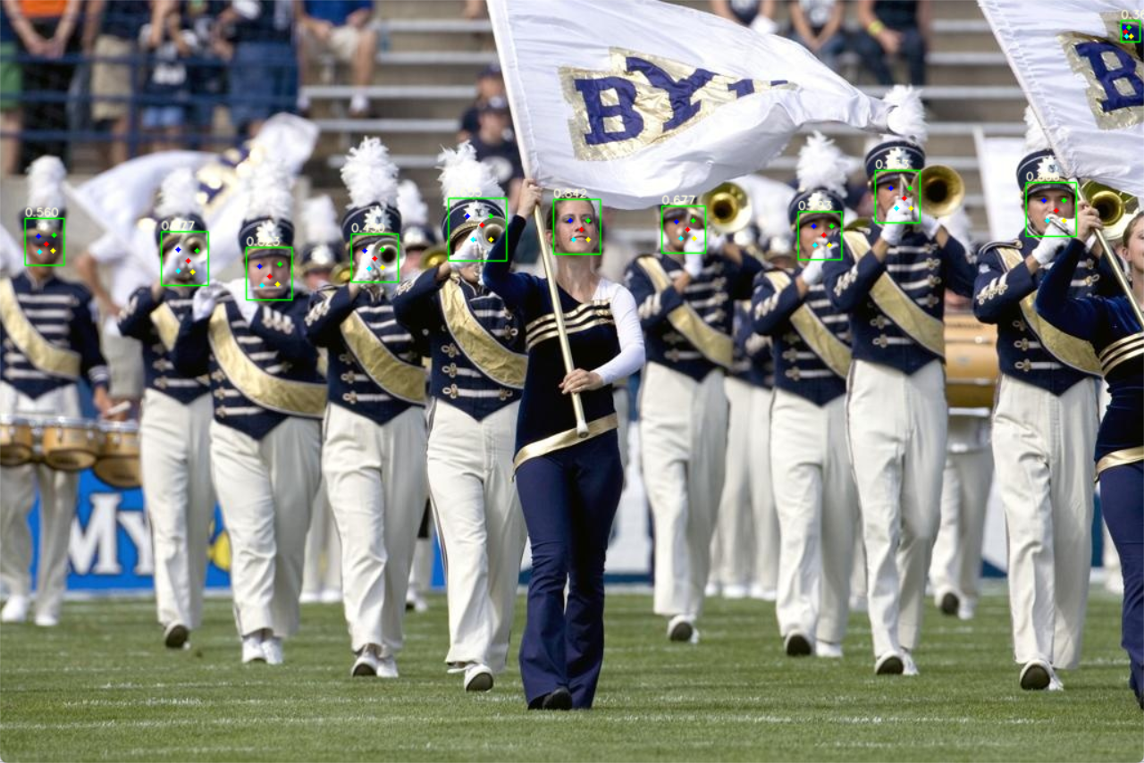
- 相关部署链接 yolov5face-toolkit
- yolov5-face-landmarks-opencv-v2
相关文章:
Yolov5-Face 原理解析及算法解析
YOLOv5-Face 文章目录 YOLOv5-Face1. 为什么人脸检测 一般检测?1.1 YOLOv5Face人脸检测1.2 YOLOv5Face Landmark 2.YOLOv5Face的设计目标和主要贡献2.1 设计目标2.2 主要贡献 3. YOLOv5Face架构3.1 模型架构3.1.1 模型示意图3.1.2 CBS模块3.1.3 Head输出3.1.4 stem…...
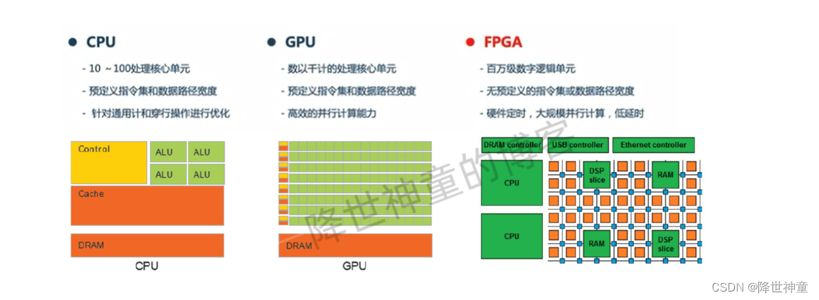
通俗易懂讲解CPU、GPU、FPGA的特点
1. CPU vs GPU 大家可以简单的将CPU理解为学识渊博的教授,什么都精通;而GPU则是一堆小学生,只会简单的算数运算。可即使教授再神通广大,也不能一秒钟内计算出500次加减法。因此,对简单重复的计算来说,单单一…...

PIC18 DataRAM 笔记
1.疑似最糟糕的英文技术文档段落 Since up to 16 registers may share the same low-order address, the user must always be careful to ensure that the proper bank is selected before performing a data read or write. For example, writing what should be program dat…...
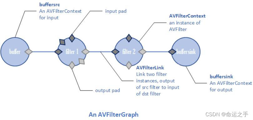
【FFMPEG】AVFilter使用流程
流程图 核心类 AVFilterGraph ⽤于统合这整个滤波过程的结构体 AVFilter 滤波器,滤波器的实现是通过AVFilter以及位于其下的结构体/函数来维护的 AVFilterContext ⼀个滤波器实例,即使是同⼀个滤波器,但是在进⾏实际的滤波时,也…...

爬虫入门06——了解cookie和session
爬虫入门06——了解cookie和session (1)什么是cookie,有什么作用 http请求是无状态的请求协议,不会记住用户的状态和信息,也不清楚你在这之前访问过什么而当网站需要记录用户是否登录时,就需要在用户登录…...

Ubuntu 的移动梦醒了
老实讲,移动版 Ubuntu 在手机、平板上的发展自始至终可能都没有达到过 Canonical 的期望,既然如此,不再勉为其难地坚持下去,或许才是更加明智的做法。 时至今日,官方显然也意识到了这一点,在早些时候发布的…...
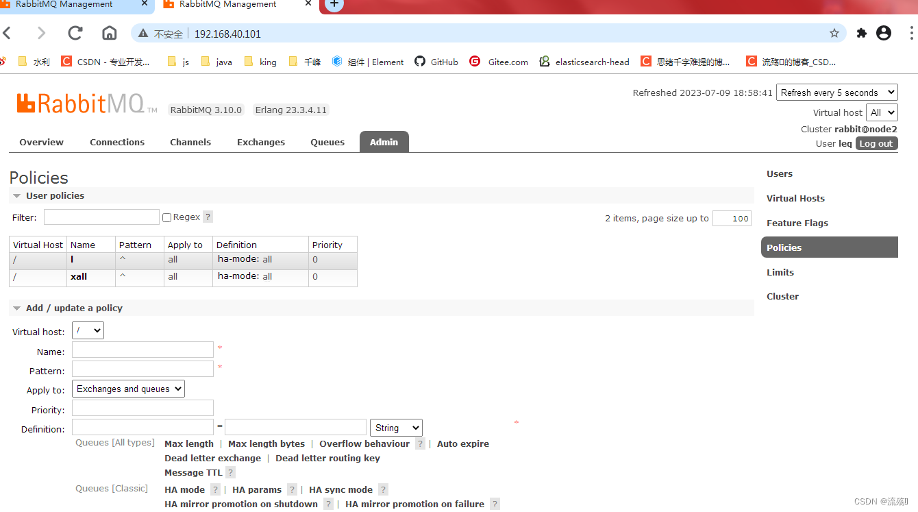
RabbitMQ的集群
新建一个虚拟机,重新安装一个RabbitMQ,不会安装的可以看下面的连接: 在Linux中安装RabbitMQ_流殇꧂的博客-CSDN博客 1.修改/etc/hosts映射文件,两台虚拟机都需要修改 vim /etc/hosts 127.0.0.1 node1 localhost.localdomain localhost4 localhost4.localdomain4 ::1 node1 loca…...
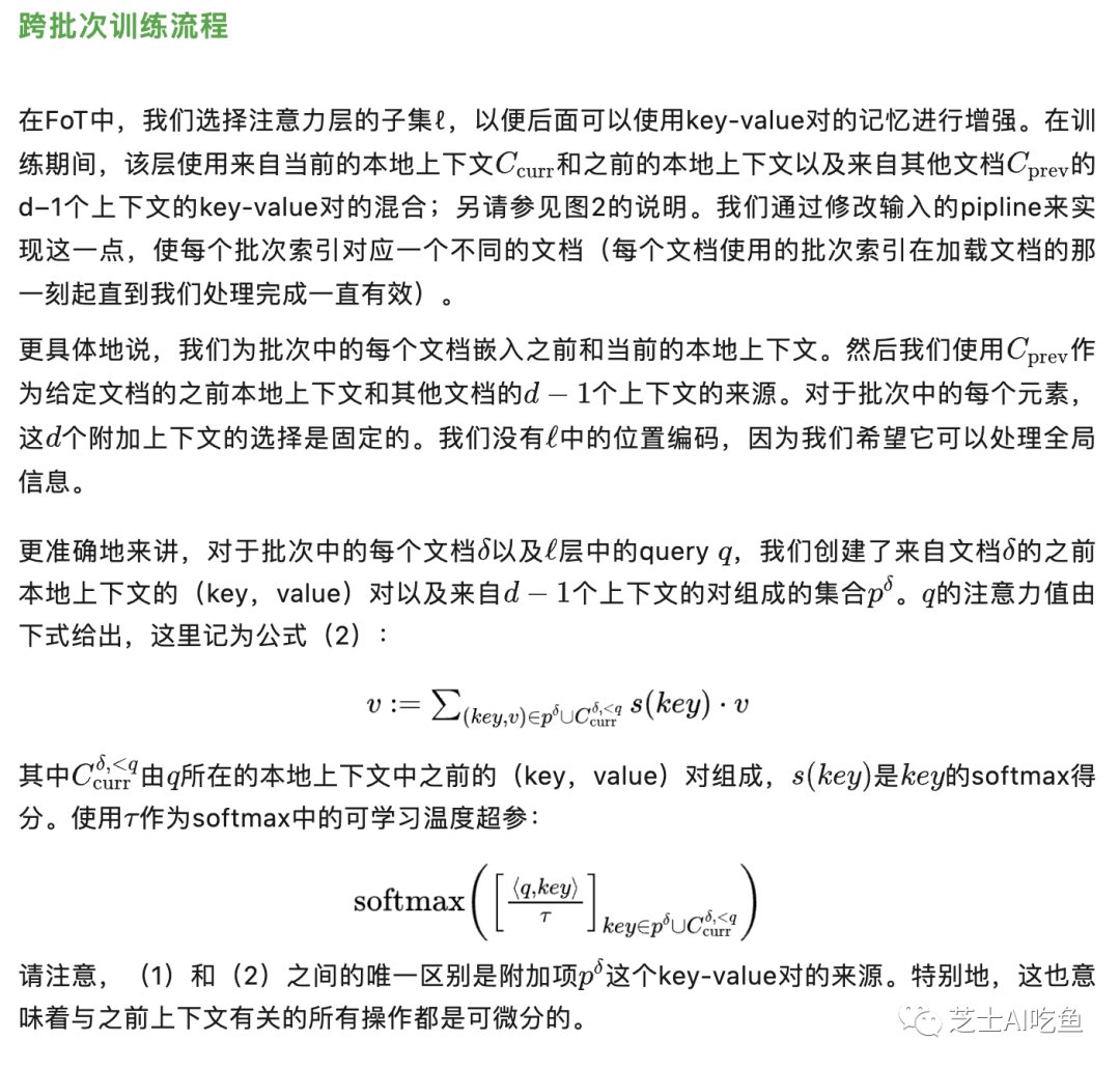
超长上下文处理:基于Transformer上下文处理常见方法梳理
原文链接:芝士AI吃鱼 目前已经采用多种方法来增加Transformer的上下文长度,主要侧重于缓解注意力计算的二次复杂度。 例如,Transformer-XL通过缓存先前的上下文,并允许随着层数的增加线性扩展上下文。Longformer采用了一种注意力…...

ChatGPT爆火 但生成式AI并非全新产物
以ChatGPT、Midjourney 为代表的 AIGC 产品横空出世,在全球掀起新一轮的 AI 技术变革新浪潮。近二十年来,我们见证了从「机器学习」算法到「深度学习」,再到「基础模型」的发展。随着数据量大规模膨胀,可扩展的算力,再…...

深度学习循环神经网络
循环神经网络(Recurrent Neural Network,RNN)是一种广泛应用于序列数据、自然语言处理等领域的神经网络。与传统的前馈神经网络不同,循环神经网络的输入不仅取决于当前输入,还取决于之前的状态。这使得循环神经网络可以…...

如何规范的设计数据库表
前言对于后端开发同学来说,访问数据库,是代码中必不可少的一个环节。系统中收集到用户的核心数据,为了安全性,我们一般会存储到数据库,比如:mysql,oracle等。后端开发的日常工作,需要…...

【CSS】跳动文字
文章目录 效果展示代码实现 效果展示 代码实现 <!DOCTYPE html> <html><head><meta charset"utf-8" /><title>一颗不甘坠落的流星</title></head><style type"text/css">/* 遮罩盒子样式 */#mask {/* 设…...

arm海思启动udev的错误
近日在配置HI3531D的文件时发现错误 random: udevd: uninitialized urandom read (16 bytes read) random: udevd: uninitialized urandom read (16 bytes read)udev 是一个为你的计算机提供设备事件的 Linux 子系统。通俗来讲就是,当你的计算机上插入了像网卡、外…...

网络协议与攻击模拟-15-DNS协议
DNS 协议 1、了解域名结构 2、 DNS 查询过程 3、在 Windows server 上部署 DNS 4、分析流量 实施 DNS 欺骗 再分析 一、 DNS 1、概念 ● DNS ( domain name system )域名系统,作为将域名的 IP 地址的相互映射关系存放在一个分布式的数据库࿰…...
ChatGPT将改变教育,而不是摧毁它
01 学校和大学的反应迅速而果断 就在 OpenAI 于 2022 年 11月下旬发布ChatGPT 的几天后,该聊天机器人被广泛谴责为一种免费的论文写作、应试工具,它很容易在作业中作弊。 美国第二大学区洛杉矶联合大学立即阻止了OpenAI网站从其学校网络访问。其他人很…...
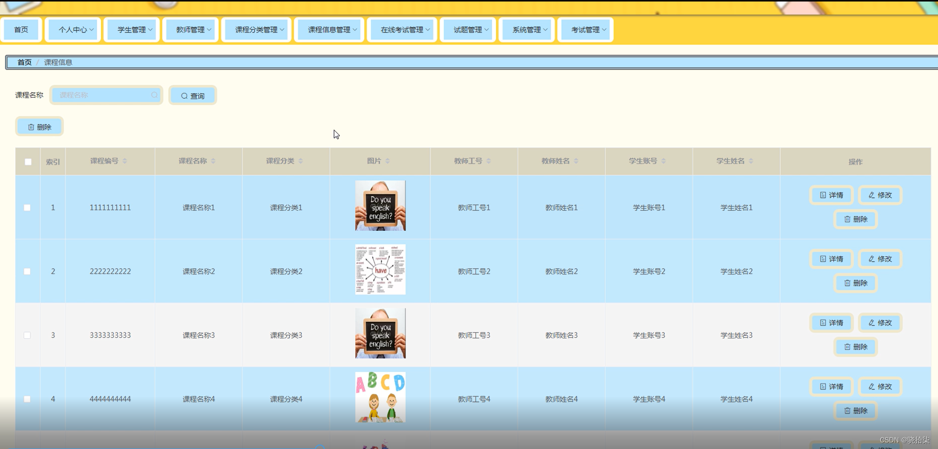
springboot在线考试
在线考试系统的开发运用java技术,MIS的总体思想,以及MYSQL等技术的支持下共同完成了该系统的开发,实现了在线考试管理的信息化,使用户体验到更优秀的在线考试管理,管理员管理操作将更加方便,实现目标....
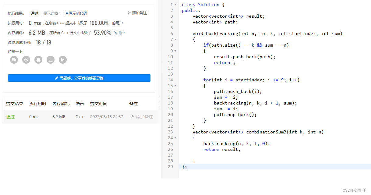
C国演义 [第三章]
第三章 组合分析步骤递归函数的返回值和参数递归结束的条件单层逻辑 组合总和 III 组合 力扣链接 给定两个整数 n 和 k,返回范围 [1, n] 中所有可能的 k 个数的组合。 你可以按 任何顺序 返回答案。 示例 1: 输入:n 4, k 2 输出࿱…...

数字化时代,企业的数据指标体系
在社会节奏越来越快,处理的信息量越来越大的今天,传统的经营管理模式已经适应不了当下的环境。而由经验、情感组成的业务调整以及决策能力不再能正确指导企业走在正确的方向上,所以数据就成为了企业新的业务优化调整和支撑企业高层管理进行决…...
三分钟了解 RocketMQ消息队列
文章目录 基本概念详细介绍主题(Topic)消息类型(MessageType)消息队列(MessageQueue)消息(Message)消息视图(MessageView)消息标签(MessageTag&am…...

golang redis第三方库github.com/go-redis/redis/v8实践
Redis基本数据类型代码示例# 这里示例使用 go-redis v8 ,不过 go-redis latest 是 v9 安装v8:go get github.com/go-redis/redis/v8 Redis 5 种基本数据类型: string 字符串类型;list列表类型;hash哈希表类型&#…...

Inner-IoU: More Effective Intersection over Union Loss with Auxiliary Bounding Box——基于辅助边界框的更有效交并比损失
这篇题为《Inner-IoU: More Effective Intersection over Union Loss with Auxiliary Bounding Box》的论文,主要研究了目标检测中边界框回归(BBR)损失函数的改进问题。以下是其核心研究内容的全面总结概括: 1. 研究背景与问题 现…...

MusePublic显存利用率提升方案:CPU卸载+自动清理策略详解
MusePublic显存利用率提升方案:CPU卸载自动清理策略详解 1. 项目背景与显存挑战 MusePublic是一款专为艺术感时尚人像创作设计的轻量化文本生成图像系统。基于专属大模型和safetensors格式封装,系统针对艺术人像的优雅姿态、细腻光影和故事感画面进行了…...
)的妙用:如何优雅地处理未使用的变量与参数)
__attribute__((unused))的妙用:如何优雅地处理未使用的变量与参数
1. 为什么我们需要__attribute__((unused)) 在C/C开发中,编译器警告就像一位严格的代码审查员,时刻提醒我们可能存在的问题。但有时候,我们确实需要定义一些暂时不使用的变量或参数,比如为了保持接口兼容性,或者在某些…...

为什么你的Jenkins构建结果不可靠?可能是工作区没清理!
为什么你的Jenkins构建结果不可靠?可能是工作区没清理! 在持续集成(CI)的实践中,Jenkins作为自动化构建的核心工具,其稳定性直接影响着开发团队的交付效率。然而,许多开发者都曾遇到过这样的困惑…...

HarmonyOS开发入门:DevEco Studio工程目录结构详解与实战配置
HarmonyOS开发实战:深度解析DevEco Studio工程架构与高效配置策略 当你第一次在DevEco Studio中创建HarmonyOS项目时,是否曾被复杂的目录结构弄得一头雾水?作为华为全场景智能生态的核心开发工具,DevEco Studio采用了一套精心设计…...

前端国际化:别让你的应用只懂一种语言
前端国际化:别让你的应用只懂一种语言 毒舌时刻这应用写得跟方言似的,出了本地就没人懂。各位前端同行,咱们今天聊聊前端国际化。别告诉我你的应用还只有中文版本,那感觉就像在国际会议上只说方言——能说,但没人懂。 …...

【人物传记】模拟单片集成电路之父-鲍勃·魏德拉
1 鲍勃魏德拉简介 鲍勃魏德拉(Bob Widlar) (1937-1991)模拟集成电路的奠基人,以μA702、μA709等开创性设计定义了模拟芯片的规则,用反叛与幽默改写了硅谷的精神,其创造的电流源、带隙基准等技术至今仍运行在每一块芯…...
)
模型航空喷气发动机CAD全套图纸(32张)
模型航空喷气发动机CAD学习资料是一套针对航空模型动力系统设计的系统性资源,涵盖从整体结构到局部零件的详细设计思路。32张图纸以标准化工程语言呈现,包含发动机外壳、燃烧室、涡轮组件、进气导管等核心模块的二维与三维视图,通过精确的线条…...

OpenClaw本地搜索增强:GLM-4.7-Flash智能文件检索系统
OpenClaw本地搜索增强:GLM-4.7-Flash智能文件检索系统 1. 为什么需要智能文件检索 作为一个长期被杂乱文件困扰的技术写作者,我经常陷入"明明记得存过某个文档却死活找不到"的困境。传统的文件名搜索就像在黑暗房间里用手电筒找东西——必须…...

3分钟从想法到3D模型:Hunyuan3D-2如何帮你实现创作自由
3分钟从想法到3D模型:Hunyuan3D-2如何帮你实现创作自由 【免费下载链接】Hunyuan3D-2 High-Resolution 3D Assets Generation with Large Scale Hunyuan3D Diffusion Models. 项目地址: https://gitcode.com/GitHub_Trending/hu/Hunyuan3D-2 想象一下&#x…...