【机器学习】Cost Function
Cost Function
- 1、计算 cost
- 2、cost 函数的直观理解
- 3、cost 可视化
- 总结
- 附录
首先,导入所需的库:
import numpy as np
%matplotlib widget
import matplotlib.pyplot as plt
from lab_utils_uni import plt_intuition, plt_stationary, plt_update_onclick, soup_bowl
plt.style.use('./deeplearning.mplstyle')
1、计算 cost
在这里,术语 ‘cost’ 是衡量模型预测房屋目标价格的程度的指标。
具有一个变量的 cost 计算公式为
J ( w , b ) = 1 2 m ∑ i = 0 m − 1 ( f w , b ( x ( i ) ) − y ( i ) ) 2 (1) J(w,b) = \frac{1}{2m} \sum\limits_{i = 0}^{m-1} (f_{w,b}(x^{(i)}) - y^{(i)})^2 \tag{1} J(w,b)=2m1i=0∑m−1(fw,b(x(i))−y(i))2(1)
其中,
f w , b ( x ( i ) ) = w x ( i ) + b (2) f_{w,b}(x^{(i)}) = wx^{(i)} + b \tag{2} fw,b(x(i))=wx(i)+b(2)
- f w , b ( x ( i ) ) f_{w,b}(x^{(i)}) fw,b(x(i)) 是使用参数 w , b w,b w,b 对样例 i i i 的预测。
- ( f w , b ( x ( i ) ) − y ( i ) ) 2 (f_{w,b}(x^{(i)}) -y^{(i)})^2 (fw,b(x(i))−y(i))2 是目标值和预测值之间的平方差。
- m m m 个样例的平方差进行相加,并除以
2m得到 cost, 即 J ( w , b ) J(w,b) J(w,b).
下面的代码通过循环每个样例来计算 cost。
def compute_cost(x, y, w, b): """Computes the cost function for linear regression.Args:x (ndarray (m,)): Data, m examples y (ndarray (m,)): target valuesw,b (scalar) : model parameters Returnstotal_cost (float): The cost of using w,b as the parameters for linear regressionto fit the data points in x and y"""# number of training examplesm = x.shape[0] cost_sum = 0 for i in range(m): f_wb = w * x[i] + b cost = (f_wb - y[i]) ** 2 cost_sum = cost_sum + cost total_cost = (1 / (2 * m)) * cost_sum return total_cost
2、cost 函数的直观理解
我们的目标是找到一个模型 f w , b ( x ) = w x + b f_{w,b}(x) = wx + b fw,b(x)=wx+b,其中 w w w 和 b b b 是参数,用于准确预测给定输入 x x x 的房屋价格。
上述 cost 计算公式(1)显示,如果可以选择 w w w 和 b b b,使得预测值 f w , b ( x ) f_{w,b}(x) fw,b(x) 与目标值 y y y 相匹配,那么 ( f w , b ( x ( i ) ) − y ( i ) ) 2 (f_{w,b}(x^{(i)}) - y^{(i)})^2 (fw,b(x(i))−y(i))2 项将为零,cost 将被最小化。
在之前的博客中,我们已经确定 b = 100 b=100 b=100 是一个最优解,所以让我们将 b b b 设为 100,并专注于 w w w。
plt_intuition(x_train,y_train)
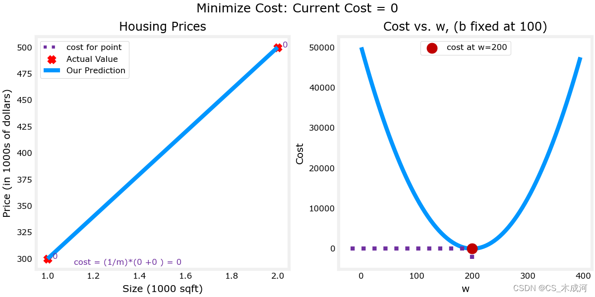
从图中可以就看出:
- 当 𝑤=200 时,cost 被最小化,这与之前博客的结果相匹配。
- 因为在 cost 计算公式中,目标值与预测值之间的差异被平方,所以当 𝑤 太大或太小时,cost 会迅速增加。
- 使用通过最小化 cost 选择的 𝑤 和 𝑏 值得到的直线与数据完美拟合。
3、cost 可视化
我们可以通过绘制3D图或使用等高线图来观察 cost 如何随着同时改变 w 和 b 而变化。
首先,定义更大的数据集
x_train = np.array([1.0, 1.7, 2.0, 2.5, 3.0, 3.2])
y_train = np.array([250, 300, 480,  430,   630, 730,])
plt.close('all')
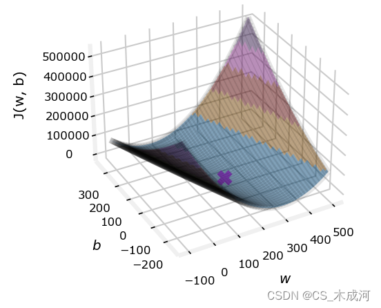
fig, ax, dyn_items = plt_stationary(x_train, y_train)
updater = plt_update_onclick(fig, ax, x_train, y_train, dyn_items)
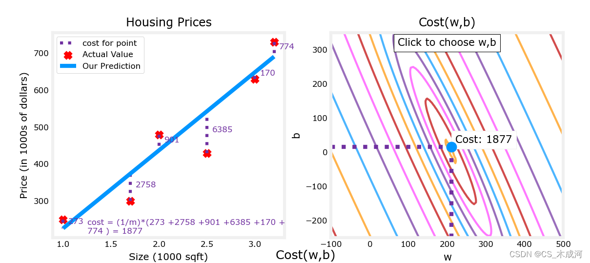
注意,因为我们的训练样例不在一条直线上,所以最小化 cost 不是0。
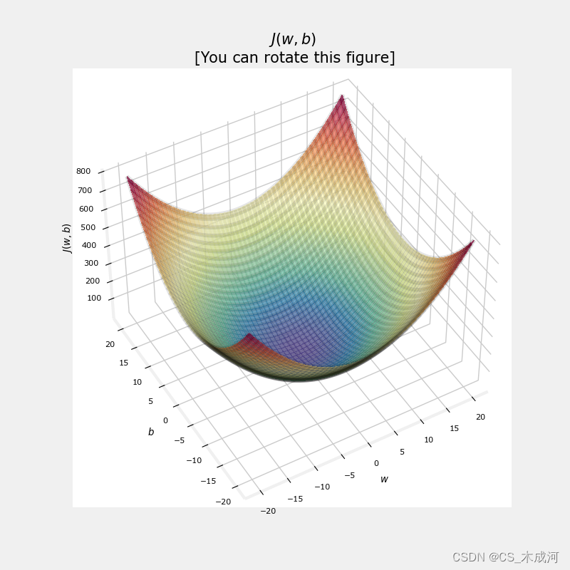
cost 函数对损失进行平方的事实确保了“误差曲面”呈现凸形,就像一个碗一样。它总会有一个通过在所有维度上追随梯度可以到达的最小值点。在之前的图中,由于 w w w 和 b b b 维度的尺度不同,这很难被察觉。下图中的 w w w 和 b b b 是对称的。
soup_bowl()
总结
- cost 计算公式提供了衡量预测与训练数据匹配程度的指标。
- 最小化 cost 可以提供参数 w w w、 b b b 的最优值。
附录
lab_utils_uni.py 源码:
"""
lab_utils_uni.pyroutines used in Course 1, Week2, labs1-3 dealing with single variables (univariate)
"""
import numpy as np
import matplotlib.pyplot as plt
from matplotlib.ticker import MaxNLocator
from matplotlib.gridspec import GridSpec
from matplotlib.colors import LinearSegmentedColormap
from ipywidgets import interact
from lab_utils_common import compute_cost
from lab_utils_common import dlblue, dlorange, dldarkred, dlmagenta, dlpurple, dlcolorsplt.style.use('./deeplearning.mplstyle')
n_bin = 5
dlcm = LinearSegmentedColormap.from_list('dl_map', dlcolors, N=n_bin)##########################################################
# Plotting Routines
##########################################################def plt_house_x(X, y,f_wb=None, ax=None):''' plot house with aXis '''if not ax:fig, ax = plt.subplots(1,1)ax.scatter(X, y, marker='x', c='r', label="Actual Value")ax.set_title("Housing Prices")ax.set_ylabel('Price (in 1000s of dollars)')ax.set_xlabel(f'Size (1000 sqft)')if f_wb is not None:ax.plot(X, f_wb,  c=dlblue, label="Our Prediction")ax.legend()def mk_cost_lines(x,y,w,b, ax):''' makes vertical cost lines'''cstr = "cost = (1/m)*("ctot = 0label = 'cost for point'addedbreak = Falsefor p in zip(x,y):f_wb_p = w*p[0]+bc_p = ((f_wb_p - p[1])**2)/2c_p_txt = c_pax.vlines(p[0], p[1],f_wb_p, lw=3, color=dlpurple, ls='dotted', label=label)label='' #just onecxy = [p[0], p[1] + (f_wb_p-p[1])/2]ax.annotate(f'{c_p_txt:0.0f}', xy=cxy, xycoords='data',color=dlpurple,xytext=(5, 0), textcoords='offset points')cstr += f"{c_p_txt:0.0f} +"if len(cstr) > 38 and addedbreak is False:cstr += "\n"addedbreak = Truectot += c_pctot = ctot/(len(x))cstr = cstr[:-1] + f") = {ctot:0.0f}"ax.text(0.15,0.02,cstr, transform=ax.transAxes, color=dlpurple)##########
# Cost lab
##########def plt_intuition(x_train, y_train):w_range = np.array([200-200,200+200])tmp_b = 100w_array = np.arange(*w_range, 5)cost = np.zeros_like(w_array)for i in range(len(w_array)):tmp_w = w_array[i]cost[i] = compute_cost(x_train, y_train, tmp_w, tmp_b)@interact(w=(*w_range,10),continuous_update=False)def func( w=150):f_wb = np.dot(x_train, w) + tmp_bfig, ax = plt.subplots(1, 2, constrained_layout=True, figsize=(8,4))fig.canvas.toolbar_position = 'bottom'mk_cost_lines(x_train, y_train, w, tmp_b, ax[0])plt_house_x(x_train, y_train, f_wb=f_wb, ax=ax[0])ax[1].plot(w_array, cost)cur_cost = compute_cost(x_train, y_train, w, tmp_b)ax[1].scatter(w,cur_cost, s=100, color=dldarkred, zorder= 10, label= f"cost at w={w}")ax[1].hlines(cur_cost, ax[1].get_xlim()[0],w, lw=4, color=dlpurple, ls='dotted')ax[1].vlines(w, ax[1].get_ylim()[0],cur_cost, lw=4, color=dlpurple, ls='dotted')ax[1].set_title("Cost vs. w, (b fixed at 100)")ax[1].set_ylabel('Cost')ax[1].set_xlabel('w')ax[1].legend(loc='upper center')fig.suptitle(f"Minimize Cost: Current Cost = {cur_cost:0.0f}", fontsize=12)plt.show()# this is the 2D cost curve with interactive slider
def plt_stationary(x_train, y_train):# setup figurefig = plt.figure( figsize=(9,8))#fig = plt.figure(constrained_layout=True,  figsize=(12,10))fig.set_facecolor('#ffffff') #whitefig.canvas.toolbar_position = 'top'#gs = GridSpec(2, 2, figure=fig, wspace = 0.01)gs = GridSpec(2, 2, figure=fig)ax0 = fig.add_subplot(gs[0, 0])ax1 = fig.add_subplot(gs[0, 1])ax2 = fig.add_subplot(gs[1, :],  projection='3d')ax = np.array([ax0,ax1,ax2])#setup useful ranges and common linspacesw_range = np.array([200-300.,200+300])b_range = np.array([50-300., 50+300])b_space  = np.linspace(*b_range, 100)w_space  = np.linspace(*w_range, 100)# get cost for w,b ranges for contour and 3Dtmp_b,tmp_w = np.meshgrid(b_space,w_space)z=np.zeros_like(tmp_b)for i in range(tmp_w.shape[0]):for j in range(tmp_w.shape[1]):z[i,j] = compute_cost(x_train, y_train, tmp_w[i][j], tmp_b[i][j] )if z[i,j] == 0: z[i,j] = 1e-6w0=200;b=-100    #initial point### plot model w cost ###f_wb = np.dot(x_train,w0) + bmk_cost_lines(x_train,y_train,w0,b,ax[0])plt_house_x(x_train, y_train, f_wb=f_wb, ax=ax[0])### plot contour ###CS = ax[1].contour(tmp_w, tmp_b, np.log(z),levels=12, linewidths=2, alpha=0.7,colors=dlcolors)ax[1].set_title('Cost(w,b)')ax[1].set_xlabel('w', fontsize=10)ax[1].set_ylabel('b', fontsize=10)ax[1].set_xlim(w_range) ; ax[1].set_ylim(b_range)cscat  = ax[1].scatter(w0,b, s=100, color=dlblue, zorder= 10, label="cost with \ncurrent w,b")chline = ax[1].hlines(b, ax[1].get_xlim()[0],w0, lw=4, color=dlpurple, ls='dotted')cvline = ax[1].vlines(w0, ax[1].get_ylim()[0],b, lw=4, color=dlpurple, ls='dotted')ax[1].text(0.5,0.95,"Click to choose w,b",  bbox=dict(facecolor='white', ec = 'black'), fontsize = 10,transform=ax[1].transAxes, verticalalignment = 'center', horizontalalignment= 'center')#Surface plot of the cost function J(w,b)ax[2].plot_surface(tmp_w, tmp_b, z,  cmap = dlcm, alpha=0.3, antialiased=True)ax[2].plot_wireframe(tmp_w, tmp_b, z, color='k', alpha=0.1)plt.xlabel("$w$")plt.ylabel("$b$")ax[2].zaxis.set_rotate_label(False)ax[2].xaxis.set_pane_color((1.0, 1.0, 1.0, 0.0))ax[2].yaxis.set_pane_color((1.0, 1.0, 1.0, 0.0))ax[2].zaxis.set_pane_color((1.0, 1.0, 1.0, 0.0))ax[2].set_zlabel("J(w, b)\n\n", rotation=90)plt.title("Cost(w,b) \n [You can rotate this figure]", size=12)ax[2].view_init(30, -120)return fig,ax, [cscat, chline, cvline]#https://matplotlib.org/stable/users/event_handling.html
class plt_update_onclick:def __init__(self, fig, ax, x_train,y_train, dyn_items):self.fig = figself.ax = axself.x_train = x_trainself.y_train = y_trainself.dyn_items = dyn_itemsself.cid = fig.canvas.mpl_connect('button_press_event', self)def __call__(self, event):if event.inaxes == self.ax[1]:ws = event.xdatabs = event.ydatacst = compute_cost(self.x_train, self.y_train, ws, bs)# clear and redraw line plotself.ax[0].clear()f_wb = np.dot(self.x_train,ws) + bsmk_cost_lines(self.x_train,self.y_train,ws,bs,self.ax[0])plt_house_x(self.x_train, self.y_train, f_wb=f_wb, ax=self.ax[0])# remove lines and re-add on countour plot and 3d plotfor artist in self.dyn_items:artist.remove()a = self.ax[1].scatter(ws,bs, s=100, color=dlblue, zorder= 10, label="cost with \ncurrent w,b")b = self.ax[1].hlines(bs, self.ax[1].get_xlim()[0],ws, lw=4, color=dlpurple, ls='dotted')c = self.ax[1].vlines(ws, self.ax[1].get_ylim()[0],bs, lw=4, color=dlpurple, ls='dotted')d = self.ax[1].annotate(f"Cost: {cst:.0f}", xy= (ws, bs), xytext = (4,4), textcoords = 'offset points',bbox=dict(facecolor='white'), size = 10)#Add point in 3D surface plote = self.ax[2].scatter3D(ws, bs,cst , marker='X', s=100)self.dyn_items = [a,b,c,d,e]self.fig.canvas.draw()def soup_bowl():""" Create figure and plot with a 3D projection"""fig = plt.figure(figsize=(8,8))#Plot configurationax = fig.add_subplot(111, projection='3d')ax.xaxis.set_pane_color((1.0, 1.0, 1.0, 0.0))ax.yaxis.set_pane_color((1.0, 1.0, 1.0, 0.0))ax.zaxis.set_pane_color((1.0, 1.0, 1.0, 0.0))ax.zaxis.set_rotate_label(False)ax.view_init(45, -120)#Useful linearspaces to give values to the parameters w and bw = np.linspace(-20, 20, 100)b = np.linspace(-20, 20, 100)#Get the z value for a bowl-shaped cost functionz=np.zeros((len(w), len(b)))j=0for x in w:i=0for y in b:z[i,j] = x**2 + y**2i+=1j+=1#Meshgrid used for plotting 3D functionsW, B = np.meshgrid(w, b)#Create the 3D surface plot of the bowl-shaped cost functionax.plot_surface(W, B, z, cmap = "Spectral_r", alpha=0.7, antialiased=False)ax.plot_wireframe(W, B, z, color='k', alpha=0.1)ax.set_xlabel("$w$")ax.set_ylabel("$b$")ax.set_zlabel("$J(w,b)$", rotation=90)ax.set_title("$J(w,b)$\n [You can rotate this figure]", size=15)plt.show()def inbounds(a,b,xlim,ylim):xlow,xhigh = xlimylow,yhigh = ylimax, ay = abx, by = bif (ax > xlow and ax < xhigh) and (bx > xlow and bx < xhigh) \and (ay > ylow and ay < yhigh) and (by > ylow and by < yhigh):return Truereturn Falsedef plt_contour_wgrad(x, y, hist, ax, w_range=[-100, 500, 5], b_range=[-500, 500, 5],contours = [0.1,50,1000,5000,10000,25000,50000],resolution=5, w_final=200, b_final=100,step=10 ):b0,w0 = np.meshgrid(np.arange(*b_range),np.arange(*w_range))z=np.zeros_like(b0)for i in range(w0.shape[0]):for j in range(w0.shape[1]):z[i][j] = compute_cost(x, y, w0[i][j], b0[i][j] )CS = ax.contour(w0, b0, z, contours, linewidths=2,colors=[dlblue, dlorange, dldarkred, dlmagenta, dlpurple])ax.clabel(CS, inline=1, fmt='%1.0f', fontsize=10)ax.set_xlabel("w");  ax.set_ylabel("b")ax.set_title('Contour plot of cost J(w,b), vs b,w with path of gradient descent')w = w_final; b=b_finalax.hlines(b, ax.get_xlim()[0],w, lw=2, color=dlpurple, ls='dotted')ax.vlines(w, ax.get_ylim()[0],b, lw=2, color=dlpurple, ls='dotted')base = hist[0]for point in hist[0::step]:edist = np.sqrt((base[0] - point[0])**2 + (base[1] - point[1])**2)if(edist > resolution or point==hist[-1]):if inbounds(point,base, ax.get_xlim(),ax.get_ylim()):plt.annotate('', xy=point, xytext=base,xycoords='data',arrowprops={'arrowstyle': '->', 'color': 'r', 'lw': 3},va='center', ha='center')base=pointreturndef plt_divergence(p_hist, J_hist, x_train,y_train):x=np.zeros(len(p_hist))y=np.zeros(len(p_hist))v=np.zeros(len(p_hist))for i in range(len(p_hist)):x[i] = p_hist[i][0]y[i] = p_hist[i][1]v[i] = J_hist[i]fig = plt.figure(figsize=(12,5))plt.subplots_adjust( wspace=0 )gs = fig.add_gridspec(1, 5)fig.suptitle(f"Cost escalates when learning rate is too large")#===============#  First subplot#===============ax = fig.add_subplot(gs[:2], )# Print w vs cost to see minimumfix_b = 100w_array = np.arange(-70000, 70000, 1000)cost = np.zeros_like(w_array)for i in range(len(w_array)):tmp_w = w_array[i]cost[i] = compute_cost(x_train, y_train, tmp_w, fix_b)ax.plot(w_array, cost)ax.plot(x,v, c=dlmagenta)ax.set_title("Cost vs w, b set to 100")ax.set_ylabel('Cost')ax.set_xlabel('w')ax.xaxis.set_major_locator(MaxNLocator(2))#===============# Second Subplot#===============tmp_b,tmp_w = np.meshgrid(np.arange(-35000, 35000, 500),np.arange(-70000, 70000, 500))z=np.zeros_like(tmp_b)for i in range(tmp_w.shape[0]):for j in range(tmp_w.shape[1]):z[i][j] = compute_cost(x_train, y_train, tmp_w[i][j], tmp_b[i][j] )ax = fig.add_subplot(gs[2:], projection='3d')ax.plot_surface(tmp_w, tmp_b, z,  alpha=0.3, color=dlblue)ax.xaxis.set_major_locator(MaxNLocator(2))ax.yaxis.set_major_locator(MaxNLocator(2))ax.set_xlabel('w', fontsize=16)ax.set_ylabel('b', fontsize=16)ax.set_zlabel('\ncost', fontsize=16)plt.title('Cost vs (b, w)')# Customize the view angleax.view_init(elev=20., azim=-65)ax.plot(x, y, v,c=dlmagenta)return# draw derivative line
# y = m*(x - x1) + y1
def add_line(dj_dx, x1, y1, d, ax):x = np.linspace(x1-d, x1+d,50)y = dj_dx*(x - x1) + y1ax.scatter(x1, y1, color=dlblue, s=50)ax.plot(x, y, '--', c=dldarkred,zorder=10, linewidth = 1)xoff = 30 if x1 == 200 else 10ax.annotate(r"$\frac{\partial J}{\partial w}$ =%d" % dj_dx, fontsize=14,xy=(x1, y1), xycoords='data',xytext=(xoff, 10), textcoords='offset points',arrowprops=dict(arrowstyle="->"),horizontalalignment='left', verticalalignment='top')def plt_gradients(x_train,y_train, f_compute_cost, f_compute_gradient):#===============#  First subplot#===============fig,ax = plt.subplots(1,2,figsize=(12,4))# Print w vs cost to see minimumfix_b = 100w_array = np.linspace(-100, 500, 50)w_array = np.linspace(0, 400, 50)cost = np.zeros_like(w_array)for i in range(len(w_array)):tmp_w = w_array[i]cost[i] = f_compute_cost(x_train, y_train, tmp_w, fix_b)ax[0].plot(w_array, cost,linewidth=1)ax[0].set_title("Cost vs w, with gradient; b set to 100")ax[0].set_ylabel('Cost')ax[0].set_xlabel('w')# plot lines for fixed b=100for tmp_w in [100,200,300]:fix_b = 100dj_dw,dj_db = f_compute_gradient(x_train, y_train, tmp_w, fix_b )j = f_compute_cost(x_train, y_train, tmp_w, fix_b)add_line(dj_dw, tmp_w, j, 30, ax[0])#===============# Second Subplot#===============tmp_b,tmp_w = np.meshgrid(np.linspace(-200, 200, 10), np.linspace(-100, 600, 10))U = np.zeros_like(tmp_w)V = np.zeros_like(tmp_b)for i in range(tmp_w.shape[0]):for j in range(tmp_w.shape[1]):U[i][j], V[i][j] = f_compute_gradient(x_train, y_train, tmp_w[i][j], tmp_b[i][j] )X = tmp_wY = tmp_bn=-2color_array = np.sqrt(((V-n)/2)**2 + ((U-n)/2)**2)ax[1].set_title('Gradient shown in quiver plot')Q = ax[1].quiver(X, Y, U, V, color_array, units='width', )ax[1].quiverkey(Q, 0.9, 0.9, 2, r'$2 \frac{m}{s}$', labelpos='E',coordinates='figure')ax[1].set_xlabel("w"); ax[1].set_ylabel("b")
相关文章:
【机器学习】Cost Function
Cost Function 1、计算 cost2、cost 函数的直观理解3、cost 可视化总结附录 首先,导入所需的库: import numpy as np %matplotlib widget import matplotlib.pyplot as plt from lab_utils_uni import plt_intuition, plt_stationary, plt_update_onclic…...
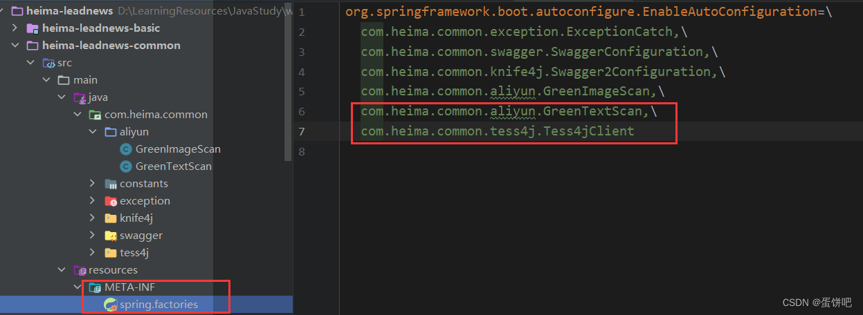
【黑马头条之内容安全第三方接口】
本笔记内容为黑马头条项目的文本-图片内容审核接口部分 目录 一、概述 二、准备工作 三、文本内容审核接口 四、图片审核接口 五、项目集成 一、概述 内容安全是识别服务,支持对图片、视频、文本、语音等对象进行多样化场景检测,有效降低内容违规风…...

回归预测 | MATLAB实现GRNN广义回归神经网络多输入单输出回归预测(多指标,多图)
回归预测 | MATLAB实现GRNN广义回归神经网络多输入单输出回归预测(多指标,多图) 目录 回归预测 | MATLAB实现GRNN广义回归神经网络多输入单输出回归预测(多指标,多图)效果一览基本介绍程序设计参考资料效果一览 基本介绍 MATLAB实现GRNN广义回归神经网络多输入单输出回归…...
详解)
STM32 HAL库函数——HAL_UART_RxCpltCallback()详解
HAL_UART_RxCpltCallback函数 他是谁,他和谁有关功能用法每收到一个字符,就自动调用一次??示例----接收未知长度的字符 他是谁,他和谁有关 HAL_UART_RxCpltCallback 是一个回调函数,用于在使用 HAL 库进行…...
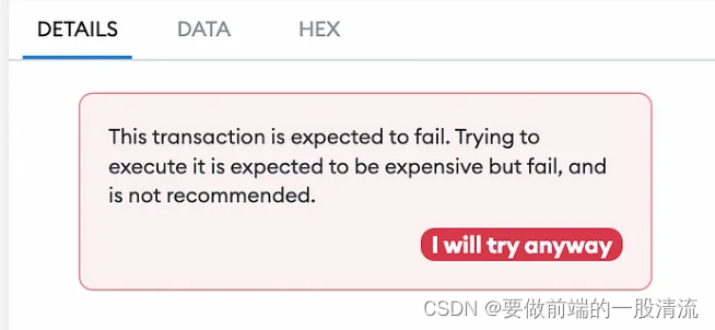
前端调用合约如何避免出现transaction fail
前言: 作为开发,你一定经历过调用合约的时候发现 gas fee 超出限制,但是不知道报了什么错。这个时候一般都是触发了require错误合约校验。对于用户来说他不理解为什么一笔交易会花费如此大的gas,那我们作为开发如何尽量避免这种情…...

选择器的使用
目录 层级选择器属性选择器伪类选择器结构伪类选择器目标伪类选择器 层级选择器 /*子代选择器:选出box下的所有li标签*/.box>li{background-color: aliceblue;}/* 选出box后面的第一个兄弟li标签 */.boxli{background-color: aliceblue;}/* 选出box后面的所有兄…...

软考A计划-系统集成项目管理工程师-项目干系人管理-上
点击跳转专栏>Unity3D特效百例点击跳转专栏>案例项目实战源码点击跳转专栏>游戏脚本-辅助自动化点击跳转专栏>Android控件全解手册点击跳转专栏>Scratch编程案例点击跳转>软考全系列点击跳转>蓝桥系列 👉关于作者 专注于Android/Unity和各种游…...
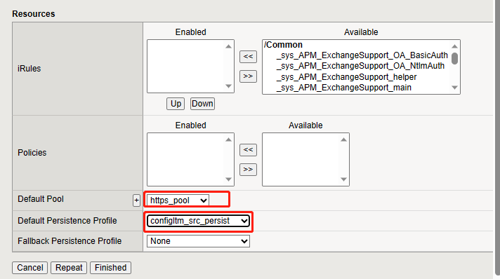
F5 LTM 知识点和实验 2-负载均衡基础概念
第二章:负载均衡基础概念 目标: 使用网页和TMSH配置virtual servers,pools,monitors,profiles和persistence等。查看统计信息 基础概念: Node一个IP地址。是创建pool池的基础。可以手工创建也可以自动创…...
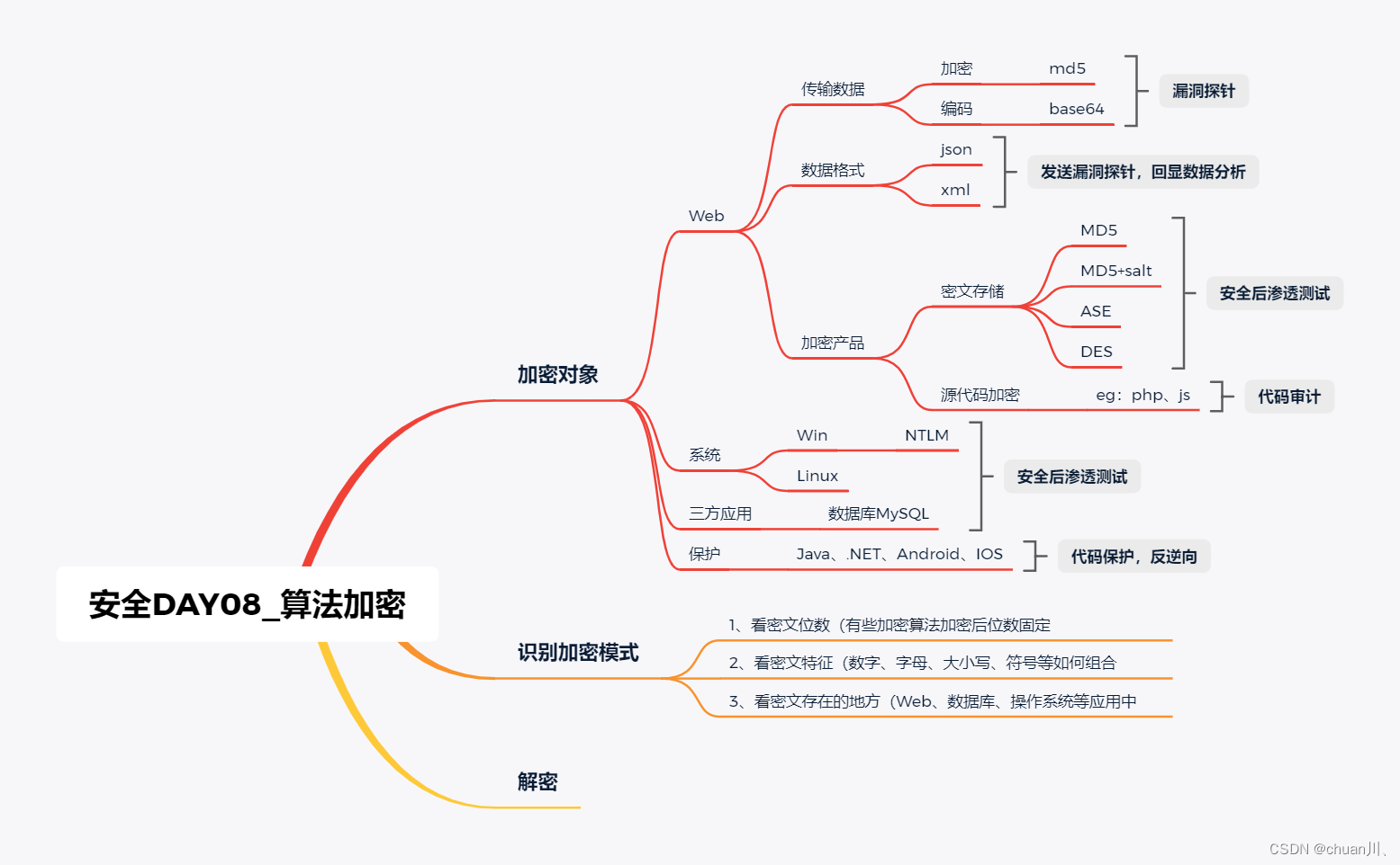
安全学习DAY08_算法加密
算法加密 漏洞分析、漏洞勘测、漏洞探针、挖漏洞时要用到的技术知识 存储密码加密-应用对象传输加密编码-发送回显数据传输格式-统一格式代码特性混淆-开发语言 传输数据 – 加密型&编码型 安全测试时,通常会进行数据的修改增加提交测试 数据在传输的时候进行…...

OpenCloudOS 与PolarDB全面适配
近日,OpenCloudOS 开源社区签署阿里巴巴开源 CLA (Contribution License Agreement, 贡献许可协议), 正式与阿里云 PolarDB 开源数据库社区牵手,并展开 OpenCloudOS (V8)与阿里云开源云原生数据库 PolarDB 分布式版、开源云原生数…...

如何在Linux系统中使用yum命令安装MySQL
1、安装软件 # yum install -y https://repo.mysql.com//mysql80-community-release-el7-8.noarch.rpm # yum -y install mysql-community-server网址来源:https://dev.mysql.com/downloads/repo/yum/ 2、启动软件 # systemctl enable mysqld# systemctl start my…...
在Ail Linux中手动配置IPv6
第一步,登录阿里云服务器控制台,在“概览”页面找到对应实例,然后单击实例ID。 第二步,在“实例详情”页面中的“网络信息”栏目中,可以发现“IPv6 地址”中没有数据,然后单击“专有网络”的专有网络ID。 第…...
TCP如何保证服务的可靠性
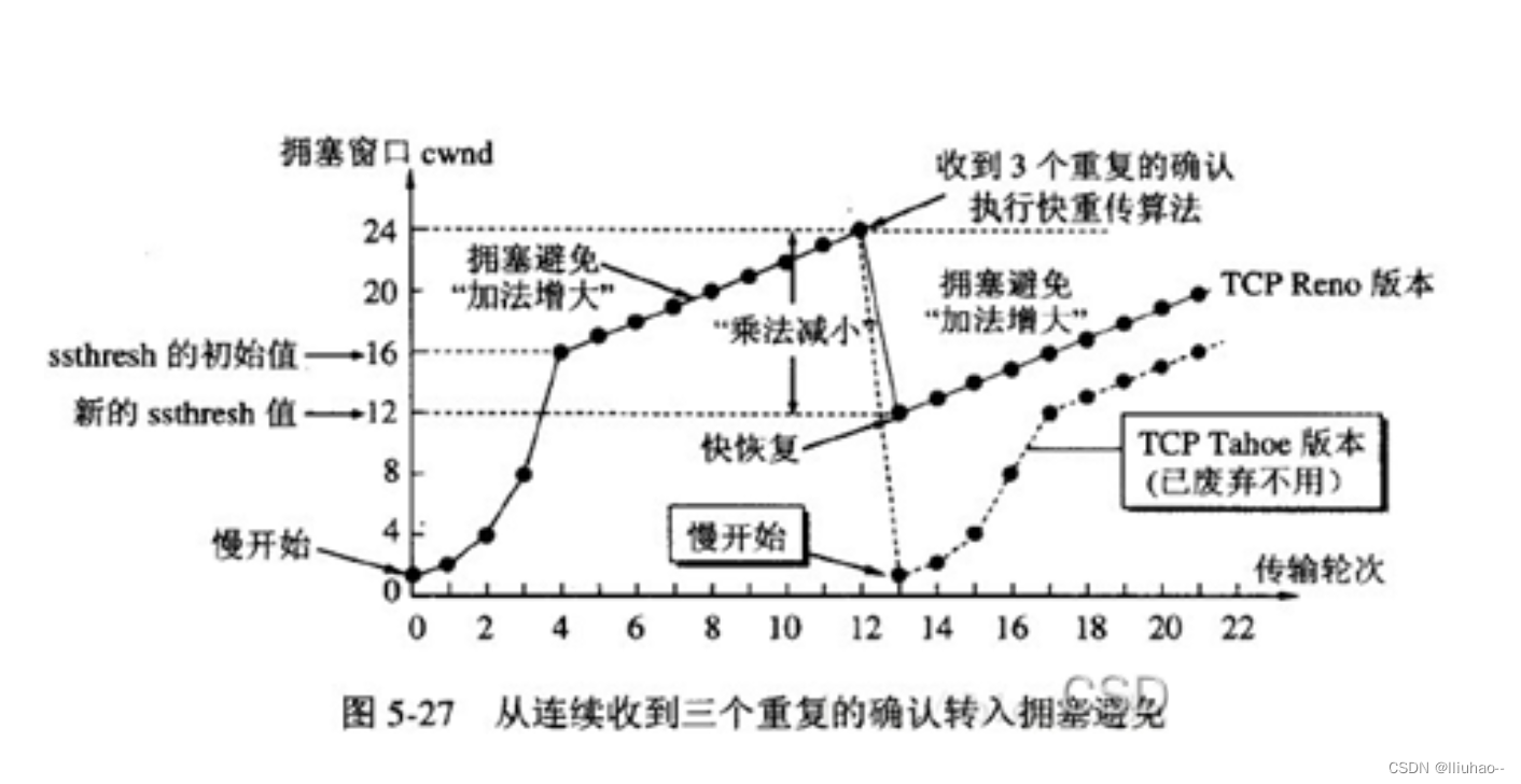
TCP如何保证服务的可靠性 确认应答超时重传流量控制滑动窗口机制概述发送窗口和接收窗口的工作原理几种滑动窗口协议1比特滑动窗口协议(停等协议)后退n协议选择重传协议 采用滑动窗口的问题(死锁可能,糊涂窗口综合征)死…...

【云原生系列】openstack搭建过程及使用
目录 搭建步骤 准备工作 正式部署OpenStack 安装的过程 安装组件如下 登录页面 进入首页 创建实例步骤 上传镜像 配置网络 服务器配置 dashboard配置 密钥配置免密登录 创建实例 绑定浮动ip 免密登录实例 搭建步骤 准备工作 1.关闭防火墙和网关 systemctl dis…...

无涯教程-jQuery - Menu组件函数
小部件菜单功能可与JqueryUI中的小部件一起使用。一个简单的菜单显示项目列表。 Menu - 语法 $( "#menu" ).menu(); Menu - 示例 以下是显示菜单用法的简单示例- <!doctype html> <html lang"en"><head><meta charset"utf-…...

Django用户登录验证和自定义验证类
一、FBV 用户登录验证 1.1 登录验证并加入 session 用户登录时,使用 authenticate 验证用户名和密码是否正确,正确则返回一个用户对象。 用户名默认的字段名是 username 密码默认的字段名是 password 将已验证的用户添加到当前会话(session)中&#x…...

json-server详解
零、文章目录 json-server详解 1、简介 Json-server 是一个零代码快速搭建本地 RESTful API 的工具。它使用 JSON 文件作为数据源,并提供了一组简单的路由和端点,可以模拟后端服务器的行为。github地址:https://github.com/typicode/json-…...
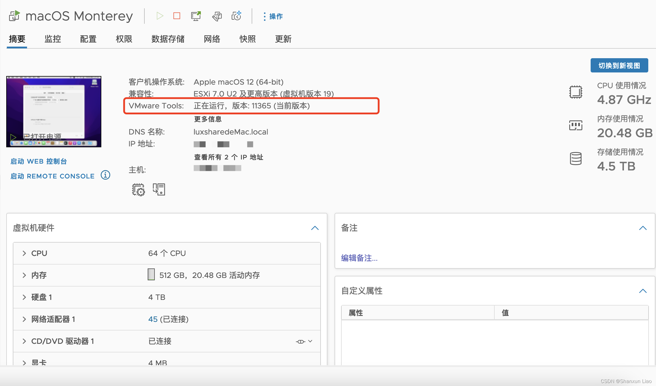
MacOS Monterey VM Install ESXi to 7 U2
一、MacOS Monterey ISO 准备 1.1 下载macOS Monterey 下载🔗链接 一定是 ISO 格式的,其他格式不适用: https://www.mediafire.com/file/4fcx0aeoehmbnmp/macOSMontereybyTechrechard.com.iso/file 1.2 将 Monterey ISO 文件上传到数据…...
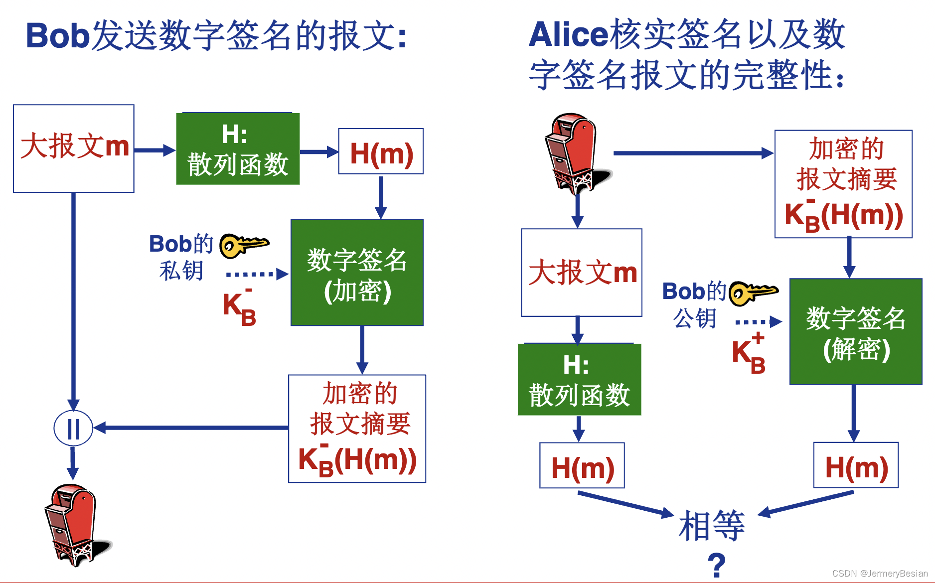
哈工大计算机网络课程网络安全基本原理详解之:消息完整性与数字签名
哈工大计算机网络课程网络安全基本原理详解之:消息完整性与数字签名 这一小节,我们继续介绍网络完全中的另一个重要内容,就是消息完整性,也为后面的数字签名打下基础。 报文完整性 首先来看一下什么是报文完整性。 报文完整性…...

K8s:K8s 20个常用命令汇总
写在前面 博文内容为节译整理,用于温习理解不足小伙伴帮忙指正 对每个人而言,真正的职责只有一个:找到自我。然后在心中坚守其一生,全心全意,永不停息。所有其它的路都是不完整的,是人的逃避方式࿰…...
)
告别串口助手:用Python脚本实现YMODEM协议自动升级嵌入式固件(附源码)
告别串口助手:用Python脚本实现YMODEM协议自动升级嵌入式固件(附源码) 在嵌入式设备量产测试和远程维护场景中,传统的手动串口工具操作已成为效率瓶颈。每次固件升级都需要人工介入,不仅耗时费力,还容易因…...

避坑指南:在Ubuntu 20.04上配置VNC远程桌面,为什么我推荐UltraVNC Viewer而不是TigerVNC?
Ubuntu 20.04远程桌面配置:为什么UltraVNC Viewer成为技术中坚的首选? 在Linux桌面环境远程管理的世界里,VNC协议就像一位历经沧桑的老兵,依然活跃在企业运维、远程开发和混合办公的第一线。Ubuntu 20.04 LTS作为长期支持版本&…...

STM32 HAL库驱动DS18B20避坑指南:单总线时序不准?试试用定时器精准延时
STM32 HAL库驱动DS18B20避坑指南:单总线时序不准?试试用定时器精准延时 在嵌入式开发中,温度传感器DS18B20因其单总线接口和数字输出特性广受欢迎。然而,许多开发者在使用STM32 HAL库驱动DS18B20时,常遇到温度读取失败…...

DeepSpeech终极指南:离线语音识别的深度学习引擎完整实践
DeepSpeech终极指南:离线语音识别的深度学习引擎完整实践 【免费下载链接】DeepSpeech DeepSpeech is an open source embedded (offline, on-device) speech-to-text engine which can run in real time on devices ranging from a Raspberry Pi 4 to high power G…...

数据可视化库对比:选择最适合你的工具
数据可视化库对比:选择最适合你的工具 前言 大家好,我是前端老炮儿。今天咱们来聊聊数据可视化库的选择! 在前端开发中,数据可视化是一个非常重要的领域。市面上有很多优秀的可视化库,比如ECharts、D3.js、Chart.js、T…...

【Midjourney新拟态风格实战指南】:20年AI视觉专家亲授7大参数调优公式与3类商业级提示词模板
更多请点击: https://intelliparadigm.com 第一章:Midjourney新拟态风格的视觉本质与演进逻辑 新拟态(Neumorphism)并非Midjourney原生支持的术语,而是社区在v6及Niji Mode迭代中通过提示词工程与风格迁移机制催生出的…...

CANN/pypto张量创建指南
Tensor的创建 【免费下载链接】pypto PyPTO(发音: pai p-t-o):Parallel Tensor/Tile Operation编程范式。 项目地址: https://gitcode.com/cann/pypto Tensor是PyPTO中的基本数据结构,用于表示将在计算图中使用并在NPU上执…...

UE5 Nanite配置指南:开启D3D12与SM6渲染管线
1. 这个提示不是报错,而是UE5在“敲你门”问你准备好了吗?刚打开UE5项目,编辑器右上角突然弹出一个黄色感叹号提示:“Nanite requires project settings to be configured for SM6 and D3D12”——很多新手第一反应是慌࿱…...

【教程】全流程基于最新导则下的生态环境影响评价技术方法及图件制作与案例实践技术应用
专题一:生态环境影响评价框架及流程 以某既包含陆域、又包含水域的项目为主要案例,兼顾其它类型项目,主要内容包括: 1、生态环境影响评价基本思路与要求:工作程序、报告编制技术要求与规范 2、资料收集与初步踏勘&a…...

奇迹 MU 荣耀出征 新区开区 最新地址官方正版下载
《奇迹 MU 荣耀出征》是正版授权的复古魔幻 MMORPG 手游,完美复刻端游 1.03H 黄金版本核心玩法,逐光娱手游官网https://www.gw648.com提供官方正规下载渠道,带你重回艾瑞西亚大陆,再续荣耀传奇。 官方正版下载渠道 《奇迹 MU 荣耀…...