【机器学习】Gradient Descent for Logistic Regression
Gradient Descent for Logistic Regression
- 1. 数据集(多变量)
- 2. 逻辑梯度下降
- 3. 梯度下降的实现及代码描述
- 3.1 计算梯度
- 3.2 梯度下降
- 4. 数据集(单变量)
- 附录
导入所需的库
import copy, math
import numpy as np
%matplotlib widget
import matplotlib.pyplot as plt
from lab_utils_common import  dlc, plot_data, plt_tumor_data, sigmoid, compute_cost_logistic
from plt_quad_logistic import plt_quad_logistic, plt_prob
plt.style.use('./deeplearning.mplstyle')
1. 数据集(多变量)
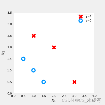
X_train = np.array([[0.5, 1.5], [1,1], [1.5, 0.5], [3, 0.5], [2, 2], [1, 2.5]])
y_train = np.array([0, 0, 0, 1, 1, 1])
fig,ax = plt.subplots(1,1,figsize=(4,4))
plot_data(X_train, y_train, ax)ax.axis([0, 4, 0, 3.5])
ax.set_ylabel('$x_1$', fontsize=12)
ax.set_xlabel('$x_0$', fontsize=12)
plt.show()
2. 逻辑梯度下降
梯度下降计算公式:
repeat until convergence: { w j = w j − α ∂ J ( w , b ) ∂ w j for j := 0..n-1 b = b − α ∂ J ( w , b ) ∂ b } \begin{align*} &\text{repeat until convergence:} \; \lbrace \\ & \; \; \;w_j = w_j - \alpha \frac{\partial J(\mathbf{w},b)}{\partial w_j} \tag{1} \; & \text{for j := 0..n-1} \\ & \; \; \; \; \;b = b - \alpha \frac{\partial J(\mathbf{w},b)}{\partial b} \\ &\rbrace \end{align*} repeat until convergence:{wj=wj−α∂wj∂J(w,b)b=b−α∂b∂J(w,b)}for j := 0..n-1(1)
其中,对于所有的 j j j 每次迭代同时更新 w j w_j wj ,
∂ J ( w , b ) ∂ w j = 1 m ∑ i = 0 m − 1 ( f w , b ( x ( i ) ) − y ( i ) ) x j ( i ) ∂ J ( w , b ) ∂ b = 1 m ∑ i = 0 m − 1 ( f w , b ( x ( i ) ) − y ( i ) ) \begin{align*} \frac{\partial J(\mathbf{w},b)}{\partial w_j} &= \frac{1}{m} \sum\limits_{i = 0}^{m-1} (f_{\mathbf{w},b}(\mathbf{x}^{(i)}) - y^{(i)})x_{j}^{(i)} \tag{2} \\ \frac{\partial J(\mathbf{w},b)}{\partial b} &= \frac{1}{m} \sum\limits_{i = 0}^{m-1} (f_{\mathbf{w},b}(\mathbf{x}^{(i)}) - y^{(i)}) \tag{3} \end{align*} ∂wj∂J(w,b)∂b∂J(w,b)=m1i=0∑m−1(fw,b(x(i))−y(i))xj(i)=m1i=0∑m−1(fw,b(x(i))−y(i))(2)(3)
- m 是训练集样例的数量
- f w , b ( x ( i ) ) f_{\mathbf{w},b}(x^{(i)}) fw,b(x(i)) 是模型预测值, y ( i ) y^{(i)} y(i) 是目标值
- 对于逻辑回归模型
z = w ⋅ x + b z = \mathbf{w} \cdot \mathbf{x} + b z=w⋅x+b
f w , b ( x ) = g ( z ) f_{\mathbf{w},b}(x) = g(z) fw,b(x)=g(z)
其中 g ( z ) g(z) g(z) 是 sigmoid 函数: g ( z ) = 1 1 + e − z g(z) = \frac{1}{1+e^{-z}} g(z)=1+e−z1
3. 梯度下降的实现及代码描述
实现梯度下降算法需要两步:
- 循环实现上面等式(1). 即下面的
gradient_descent - 当前梯度的计算等式(2, 3). 即下面的
compute_gradient_logistic
3.1 计算梯度
对于所有的 w j w_j wj 和 b b b,实现等式 (2),(3)
-
初始化变量计算
dj_dw和dj_db -
对每个样例:
- 计算误差 g ( w ⋅ x ( i ) + b ) − y ( i ) g(\mathbf{w} \cdot \mathbf{x}^{(i)} + b) - \mathbf{y}^{(i)} g(w⋅x(i)+b)−y(i)
- 对于这个样例中的每个输入值 x j ( i ) x_{j}^{(i)} xj(i) ,
- 误差乘以输入值 x j ( i ) x_{j}^{(i)} xj(i), 然后加到对应的
dj_dw中. (上述等式2)
- 误差乘以输入值 x j ( i ) x_{j}^{(i)} xj(i), 然后加到对应的
- 累加误差到
dj_db(上述等式3)
-
dj_db和dj_dw都除以样例总数 m m m -
在Numpy中 x ( i ) \mathbf{x}^{(i)} x(i) 是
X[i,:]或者X[i], x j ( i ) x_{j}^{(i)} xj(i) 是X[i,j]
代码描述:
def compute_gradient_logistic(X, y, w, b): """Computes the gradient for linear regression Args:X (ndarray (m,n): Data, m examples with n featuresy (ndarray (m,)): target valuesw (ndarray (n,)): model parameters b (scalar) : model parameterReturnsdj_dw (ndarray (n,)): The gradient of the cost w.r.t. the parameters w. dj_db (scalar) : The gradient of the cost w.r.t. the parameter b. """m,n = X.shapedj_dw = np.zeros((n,)) #(n,)dj_db = 0.for i in range(m):f_wb_i = sigmoid(np.dot(X[i],w) + b) #(n,)(n,)=scalarerr_i = f_wb_i - y[i] #scalarfor j in range(n):dj_dw[j] = dj_dw[j] + err_i * X[i,j] #scalardj_db = dj_db + err_idj_dw = dj_dw/m #(n,)dj_db = dj_db/m #scalarreturn dj_db, dj_dw
测试一下
X_tmp = np.array([[0.5, 1.5], [1,1], [1.5, 0.5], [3, 0.5], [2, 2], [1, 2.5]])
y_tmp = np.array([0, 0, 0, 1, 1, 1])
w_tmp = np.array([2.,3.])
b_tmp = 1.
dj_db_tmp, dj_dw_tmp = compute_gradient_logistic(X_tmp, y_tmp, w_tmp, b_tmp)
print(f"dj_db: {dj_db_tmp}" )
print(f"dj_dw: {dj_dw_tmp.tolist()}" )

3.2 梯度下降
实现上述公式(1),代码为:
def gradient_descent(X, y, w_in, b_in, alpha, num_iters): """Performs batch gradient descentArgs:X (ndarray (m,n) : Data, m examples with n featuresy (ndarray (m,)) : target valuesw_in (ndarray (n,)): Initial values of model parameters b_in (scalar) : Initial values of model parameteralpha (float) : Learning ratenum_iters (scalar) : number of iterations to run gradient descentReturns:w (ndarray (n,)) : Updated values of parametersb (scalar) : Updated value of parameter """# An array to store cost J and w's at each iteration primarily for graphing laterJ_history = []w = copy.deepcopy(w_in) #avoid modifying global w within functionb = b_infor i in range(num_iters):# Calculate the gradient and update the parametersdj_db, dj_dw = compute_gradient_logistic(X, y, w, b) # Update Parameters using w, b, alpha and gradientw = w - alpha * dj_dw b = b - alpha * dj_db # Save cost J at each iterationif i<100000: # prevent resource exhaustion J_history.append( compute_cost_logistic(X, y, w, b) )# Print cost every at intervals 10 times or as many iterations if < 10if i% math.ceil(num_iters / 10) == 0:print(f"Iteration {i:4d}: Cost {J_history[-1]} ")return w, b, J_history #return final w,b and J history for graphing
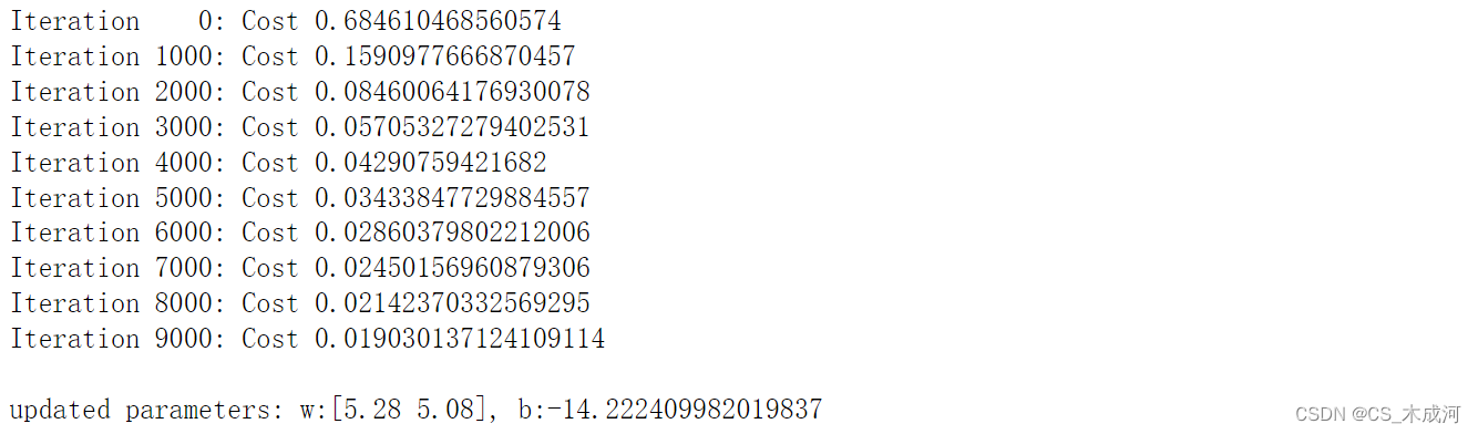
运行一下:
w_tmp  = np.zeros_like(X_train[0])
b_tmp  = 0.
alph = 0.1
iters = 10000w_out, b_out, _ = gradient_descent(X_train, y_train, w_tmp, b_tmp, alph, iters)
print(f"\nupdated parameters: w:{w_out}, b:{b_out}")
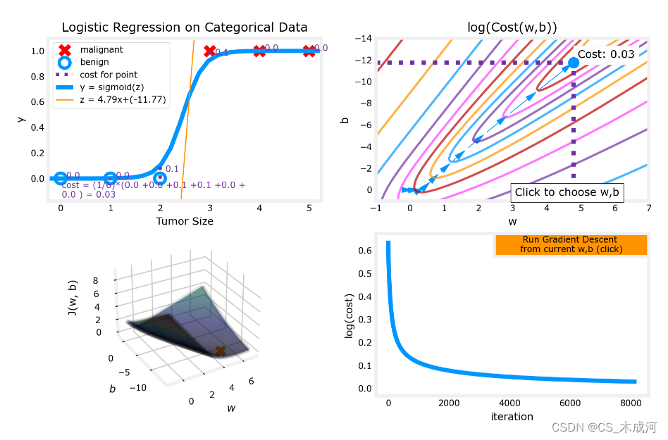
梯度下降的结果可视化:
fig,ax = plt.subplots(1,1,figsize=(5,4))
# plot the probability
plt_prob(ax, w_out, b_out)# Plot the original data
ax.set_ylabel(r'$x_1$')
ax.set_xlabel(r'$x_0$')
ax.axis([0, 4, 0, 3.5])
plot_data(X_train,y_train,ax)# Plot the decision boundary
x0 = -b_out/w_out[1]
x1 = -b_out/w_out[0]
ax.plot([0,x0],[x1,0], c=dlc["dlblue"], lw=1)
plt.show()
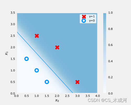
在上图中,阴影部分表示概率 y=1,决策边界是概率为0.5的直线。
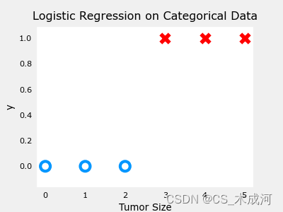
4. 数据集(单变量)
导入数据绘图可视化,此时参数为 w w w, b b b:
x_train = np.array([0., 1, 2, 3, 4, 5])
y_train = np.array([0,  0, 0, 1, 1, 1])fig,ax = plt.subplots(1,1,figsize=(4,3))
plt_tumor_data(x_train, y_train, ax)
plt.show()
w_range = np.array([-1, 7])
b_range = np.array([1, -14])
quad = plt_quad_logistic( x_train, y_train, w_range, b_range )
附录
lab_utils_common.py 源码:
"""
lab_utils_commoncontains common routines and variable definitionsused by all the labs in this week.by contrast, specific, large plotting routines will be in separate filesand are generally imported into the week where they are used.those files will import this file
"""
import copy
import math
import numpy as np
import matplotlib.pyplot as plt
from matplotlib.patches import FancyArrowPatch
from ipywidgets import Outputnp.set_printoptions(precision=2)dlc = dict(dlblue = '#0096ff', dlorange = '#FF9300', dldarkred='#C00000', dlmagenta='#FF40FF', dlpurple='#7030A0')
dlblue = '#0096ff'; dlorange = '#FF9300'; dldarkred='#C00000'; dlmagenta='#FF40FF'; dlpurple='#7030A0'
dlcolors = [dlblue, dlorange, dldarkred, dlmagenta, dlpurple]
plt.style.use('./deeplearning.mplstyle')def sigmoid(z):"""Compute the sigmoid of zParameters----------z : array_likeA scalar or numpy array of any size.Returns-------g : array_likesigmoid(z)"""z = np.clip( z, -500, 500 )           # protect against overflowg = 1.0/(1.0+np.exp(-z))return g##########################################################
# Regression Routines
##########################################################def predict_logistic(X, w, b):""" performs prediction """return sigmoid(X @ w + b)def predict_linear(X, w, b):""" performs prediction """return X @ w + bdef compute_cost_logistic(X, y, w, b, lambda_=0, safe=False):"""Computes cost using logistic loss, non-matrix versionArgs:X (ndarray): Shape (m,n)  matrix of examples with n featuresy (ndarray): Shape (m,)   target valuesw (ndarray): Shape (n,)   parameters for predictionb (scalar):               parameter  for predictionlambda_ : (scalar, float) Controls amount of regularization, 0 = no regularizationsafe : (boolean)          True-selects under/overflow safe algorithmReturns:cost (scalar): cost"""m,n = X.shapecost = 0.0for i in range(m):z_i    = np.dot(X[i],w) + b                                             #(n,)(n,) or (n,) ()if safe:  #avoids overflowscost += -(y[i] * z_i ) + log_1pexp(z_i)else:f_wb_i = sigmoid(z_i)                                                   #(n,)cost  += -y[i] * np.log(f_wb_i) - (1 - y[i]) * np.log(1 - f_wb_i)       # scalarcost = cost/mreg_cost = 0if lambda_ != 0:for j in range(n):reg_cost += (w[j]**2)                                               # scalarreg_cost = (lambda_/(2*m))*reg_costreturn cost + reg_costdef log_1pexp(x, maximum=20):''' approximate log(1+exp^x)https://stats.stackexchange.com/questions/475589/numerical-computation-of-cross-entropy-in-practiceArgs:x   : (ndarray Shape (n,1) or (n,)  inputout : (ndarray Shape matches x      output ~= np.log(1+exp(x))'''out  = np.zeros_like(x,dtype=float)i    = x <= maximumni   = np.logical_not(i)out[i]  = np.log(1 + np.exp(x[i]))out[ni] = x[ni]return outdef compute_cost_matrix(X, y, w, b, logistic=False, lambda_=0, safe=True):"""Computes the cost using  using matricesArgs:X : (ndarray, Shape (m,n))          matrix of examplesy : (ndarray  Shape (m,) or (m,1))  target value of each examplew : (ndarray  Shape (n,) or (n,1))  Values of parameter(s) of the modelb : (scalar )                       Values of parameter of the modelverbose : (Boolean) If true, print out intermediate value f_wbReturns:total_cost: (scalar)                cost"""m = X.shape[0]y = y.reshape(-1,1)             # ensure 2Dw = w.reshape(-1,1)             # ensure 2Dif logistic:if safe:  #safe from overflowz = X @ w + b                                                           #(m,n)(n,1)=(m,1)cost = -(y * z) + log_1pexp(z)cost = np.sum(cost)/m                                                   # (scalar)else:f    = sigmoid(X @ w + b)                                               # (m,n)(n,1) = (m,1)cost = (1/m)*(np.dot(-y.T, np.log(f)) - np.dot((1-y).T, np.log(1-f)))   # (1,m)(m,1) = (1,1)cost = cost[0,0]                                                        # scalarelse:f    = X @ w + b                                                        # (m,n)(n,1) = (m,1)cost = (1/(2*m)) * np.sum((f - y)**2)                                   # scalarreg_cost = (lambda_/(2*m)) * np.sum(w**2)                                   # scalartotal_cost = cost + reg_cost                                                # scalarreturn total_cost                                                           # scalardef compute_gradient_matrix(X, y, w, b, logistic=False, lambda_=0):"""Computes the gradient using matricesArgs:X : (ndarray, Shape (m,n))          matrix of examplesy : (ndarray  Shape (m,) or (m,1))  target value of each examplew : (ndarray  Shape (n,) or (n,1))  Values of parameters of the modelb : (scalar )                       Values of parameter of the modellogistic: (boolean)                 linear if false, logistic if truelambda_:  (float)                   applies regularization if non-zeroReturnsdj_dw: (array_like Shape (n,1))     The gradient of the cost w.r.t. the parameters wdj_db: (scalar)                     The gradient of the cost w.r.t. the parameter b"""m = X.shape[0]y = y.reshape(-1,1)             # ensure 2Dw = w.reshape(-1,1)             # ensure 2Df_wb  = sigmoid( X @ w + b ) if logistic else  X @ w + b      # (m,n)(n,1) = (m,1)err   = f_wb - y                                              # (m,1)dj_dw = (1/m) * (X.T @ err)                                   # (n,m)(m,1) = (n,1)dj_db = (1/m) * np.sum(err)                                   # scalardj_dw += (lambda_/m) * w        # regularize                  # (n,1)return dj_db, dj_dw                                           # scalar, (n,1)def gradient_descent(X, y, w_in, b_in, alpha, num_iters, logistic=False, lambda_=0, verbose=True):"""Performs batch gradient descent to learn theta. Updates theta by takingnum_iters gradient steps with learning rate alphaArgs:X (ndarray):    Shape (m,n)         matrix of examplesy (ndarray):    Shape (m,) or (m,1) target value of each examplew_in (ndarray): Shape (n,) or (n,1) Initial values of parameters of the modelb_in (scalar):                      Initial value of parameter of the modellogistic: (boolean)                 linear if false, logistic if truelambda_:  (float)                   applies regularization if non-zeroalpha (float):                      Learning ratenum_iters (int):                    number of iterations to run gradient descentReturns:w (ndarray): Shape (n,) or (n,1)    Updated values of parameters; matches incoming shapeb (scalar):                         Updated value of parameter"""# An array to store cost J and w's at each iteration primarily for graphing laterJ_history = []w = copy.deepcopy(w_in)  #avoid modifying global w within functionb = b_inw = w.reshape(-1,1)      #prep for matrix operationsy = y.reshape(-1,1)for i in range(num_iters):# Calculate the gradient and update the parametersdj_db,dj_dw = compute_gradient_matrix(X, y, w, b, logistic, lambda_)# Update Parameters using w, b, alpha and gradientw = w - alpha * dj_dwb = b - alpha * dj_db# Save cost J at each iterationif i<100000:      # prevent resource exhaustionJ_history.append( compute_cost_matrix(X, y, w, b, logistic, lambda_) )# Print cost every at intervals 10 times or as many iterations if < 10if i% math.ceil(num_iters / 10) == 0:if verbose: print(f"Iteration {i:4d}: Cost {J_history[-1]}   ")return w.reshape(w_in.shape), b, J_history  #return final w,b and J history for graphingdef zscore_normalize_features(X):"""computes  X, zcore normalized by columnArgs:X (ndarray): Shape (m,n) input data, m examples, n featuresReturns:X_norm (ndarray): Shape (m,n)  input normalized by columnmu (ndarray):     Shape (n,)   mean of each featuresigma (ndarray):  Shape (n,)   standard deviation of each feature"""# find the mean of each column/featuremu     = np.mean(X, axis=0)                 # mu will have shape (n,)# find the standard deviation of each column/featuresigma  = np.std(X, axis=0)                  # sigma will have shape (n,)# element-wise, subtract mu for that column from each example, divide by std for that columnX_norm = (X - mu) / sigmareturn X_norm, mu, sigma#check our work
#from sklearn.preprocessing import scale
#scale(X_orig, axis=0, with_mean=True, with_std=True, copy=True)######################################################
# Common Plotting Routines
######################################################def plot_data(X, y, ax, pos_label="y=1", neg_label="y=0", s=80, loc='best' ):""" plots logistic data with two axis """# Find Indices of Positive and Negative Examplespos = y == 1neg = y == 0pos = pos.reshape(-1,)  #work with 1D or 1D y vectorsneg = neg.reshape(-1,)# Plot examplesax.scatter(X[pos, 0], X[pos, 1], marker='x', s=s, c = 'red', label=pos_label)ax.scatter(X[neg, 0], X[neg, 1], marker='o', s=s, label=neg_label, facecolors='none', edgecolors=dlblue, lw=3)ax.legend(loc=loc)ax.figure.canvas.toolbar_visible = Falseax.figure.canvas.header_visible = Falseax.figure.canvas.footer_visible = Falsedef plt_tumor_data(x, y, ax):""" plots tumor data on one axis """pos = y == 1neg = y == 0ax.scatter(x[pos], y[pos], marker='x', s=80, c = 'red', label="malignant")ax.scatter(x[neg], y[neg], marker='o', s=100, label="benign", facecolors='none', edgecolors=dlblue,lw=3)ax.set_ylim(-0.175,1.1)ax.set_ylabel('y')ax.set_xlabel('Tumor Size')ax.set_title("Logistic Regression on Categorical Data")ax.figure.canvas.toolbar_visible = Falseax.figure.canvas.header_visible = Falseax.figure.canvas.footer_visible = False# Draws a threshold at 0.5
def draw_vthresh(ax,x):""" draws a threshold """ylim = ax.get_ylim()xlim = ax.get_xlim()ax.fill_between([xlim[0], x], [ylim[1], ylim[1]], alpha=0.2, color=dlblue)ax.fill_between([x, xlim[1]], [ylim[1], ylim[1]], alpha=0.2, color=dldarkred)ax.annotate("z >= 0", xy= [x,0.5], xycoords='data',xytext=[30,5],textcoords='offset points')d = FancyArrowPatch(posA=(x, 0.5), posB=(x+3, 0.5), color=dldarkred,arrowstyle='simple, head_width=5, head_length=10, tail_width=0.0',)ax.add_artist(d)ax.annotate("z < 0", xy= [x,0.5], xycoords='data',xytext=[-50,5],textcoords='offset points', ha='left')f = FancyArrowPatch(posA=(x, 0.5), posB=(x-3, 0.5), color=dlblue,arrowstyle='simple, head_width=5, head_length=10, tail_width=0.0',)ax.add_artist(f)
plt_quad_logistic.py 源码:
"""
plt_quad_logistic.pyinteractive plot and supporting routines showing logistic regression
"""import time
from matplotlib import cm
import matplotlib.colors as colors
from matplotlib.gridspec import GridSpec
from matplotlib.widgets import Button
from matplotlib.patches import FancyArrowPatch
from ipywidgets import Output
from lab_utils_common import np, plt, dlc, dlcolors, sigmoid, compute_cost_matrix, gradient_descent# for debug
#output = Output() # sends hidden error messages to display when using widgets
#display(output)class plt_quad_logistic:''' plots a quad plot showing logistic regression '''# pylint: disable=too-many-instance-attributes# pylint: disable=too-many-locals# pylint: disable=missing-function-docstring# pylint: disable=attribute-defined-outside-initdef __init__(self, x_train,y_train, w_range, b_range):# setup figurefig = plt.figure( figsize=(10,6))fig.canvas.toolbar_visible = Falsefig.canvas.header_visible = Falsefig.canvas.footer_visible = Falsefig.set_facecolor('#ffffff') #whitegs  = GridSpec(2, 2, figure=fig)ax0 = fig.add_subplot(gs[0, 0])ax1 = fig.add_subplot(gs[0, 1])ax2 = fig.add_subplot(gs[1, 0],  projection='3d')ax3 = fig.add_subplot(gs[1,1])pos = ax3.get_position().get_points()  ##[[lb_x,lb_y], [rt_x, rt_y]]h = 0.05 width = 0.2axcalc   = plt.axes([pos[1,0]-width, pos[1,1]-h, width, h])  #lx,by,w,hax = np.array([ax0, ax1, ax2, ax3, axcalc])self.fig = figself.ax = axself.x_train = x_trainself.y_train = y_trainself.w = 0. #initial point, non-arrayself.b = 0.# initialize subplotsself.dplot = data_plot(ax[0], x_train, y_train, self.w, self.b)self.con_plot = contour_and_surface_plot(ax[1], ax[2], x_train, y_train, w_range, b_range, self.w, self.b)self.cplot = cost_plot(ax[3])# setup eventsself.cid = fig.canvas.mpl_connect('button_press_event', self.click_contour)self.bcalc = Button(axcalc, 'Run Gradient Descent \nfrom current w,b (click)', color=dlc["dlorange"])self.bcalc.on_clicked(self.calc_logistic)#    @output.capture()  # debugdef click_contour(self, event):''' called when click in contour '''if event.inaxes == self.ax[1]:   #contour plotself.w = event.xdataself.b = event.ydataself.cplot.re_init()self.dplot.update(self.w, self.b)self.con_plot.update_contour_wb_lines(self.w, self.b)self.con_plot.path.re_init(self.w, self.b)self.fig.canvas.draw()#    @output.capture()  # debugdef calc_logistic(self, event):''' called on run gradient event '''for it in [1, 8,16,32,64,128,256,512,1024,2048,4096]:w, self.b, J_hist = gradient_descent(self.x_train.reshape(-1,1), self.y_train.reshape(-1,1),np.array(self.w).reshape(-1,1), self.b, 0.1, it,logistic=True, lambda_=0, verbose=False)self.w = w[0,0]self.dplot.update(self.w, self.b)self.con_plot.update_contour_wb_lines(self.w, self.b)self.con_plot.path.add_path_item(self.w,self.b)self.cplot.add_cost(J_hist)time.sleep(0.3)self.fig.canvas.draw()class data_plot:''' handles data plot '''# pylint: disable=missing-function-docstring# pylint: disable=attribute-defined-outside-initdef __init__(self, ax, x_train, y_train, w, b):self.ax = axself.x_train = x_trainself.y_train = y_trainself.m = x_train.shape[0]self.w = wself.b = bself.plt_tumor_data()self.draw_logistic_lines(firsttime=True)self.mk_cost_lines(firsttime=True)self.ax.autoscale(enable=False) # leave plot scales the same after initial setupdef plt_tumor_data(self):x = self.x_trainy = self.y_trainpos = y == 1neg = y == 0self.ax.scatter(x[pos], y[pos], marker='x', s=80, c = 'red', label="malignant")self.ax.scatter(x[neg], y[neg], marker='o', s=100, label="benign", facecolors='none',edgecolors=dlc["dlblue"],lw=3)self.ax.set_ylim(-0.175,1.1)self.ax.set_ylabel('y')self.ax.set_xlabel('Tumor Size')self.ax.set_title("Logistic Regression on Categorical Data")def update(self, w, b):self.w = wself.b = bself.draw_logistic_lines()self.mk_cost_lines()def draw_logistic_lines(self, firsttime=False):if not firsttime:self.aline[0].remove()self.bline[0].remove()self.alegend.remove()xlim  = self.ax.get_xlim()x_hat = np.linspace(*xlim, 30)y_hat = sigmoid(np.dot(x_hat.reshape(-1,1), self.w) + self.b)self.aline = self.ax.plot(x_hat, y_hat, color=dlc["dlblue"],label="y = sigmoid(z)")f_wb = np.dot(x_hat.reshape(-1,1), self.w) + self.bself.bline = self.ax.plot(x_hat, f_wb, color=dlc["dlorange"], lw=1,label=f"z = {np.squeeze(self.w):0.2f}x+({self.b:0.2f})")self.alegend = self.ax.legend(loc='upper left')def mk_cost_lines(self, firsttime=False):''' makes vertical cost lines'''if not firsttime:for artist in self.cost_items:artist.remove()self.cost_items = []cstr = f"cost = (1/{self.m})*("ctot = 0label = 'cost for point'addedbreak = Falsefor p in zip(self.x_train,self.y_train):f_wb_p = sigmoid(self.w*p[0]+self.b)c_p = compute_cost_matrix(p[0].reshape(-1,1), p[1],np.array(self.w), self.b, logistic=True, lambda_=0, safe=True)c_p_txt = c_pa = self.ax.vlines(p[0], p[1],f_wb_p, lw=3, color=dlc["dlpurple"], ls='dotted', label=label)label='' #just onecxy = [p[0], p[1] + (f_wb_p-p[1])/2]b = self.ax.annotate(f'{c_p_txt:0.1f}', xy=cxy, xycoords='data',color=dlc["dlpurple"],xytext=(5, 0), textcoords='offset points')cstr += f"{c_p_txt:0.1f} +"if len(cstr) > 38 and addedbreak is False:cstr += "\n"addedbreak = Truectot += c_pself.cost_items.extend((a,b))ctot = ctot/(len(self.x_train))cstr = cstr[:-1] + f") = {ctot:0.2f}"## todo.. figure out how to get this textbox to extend to the width of the subplotc = self.ax.text(0.05,0.02,cstr, transform=self.ax.transAxes, color=dlc["dlpurple"])self.cost_items.append(c)class contour_and_surface_plot:''' plots combined in class as they have similar operations '''# pylint: disable=missing-function-docstring# pylint: disable=attribute-defined-outside-initdef __init__(self, axc, axs, x_train, y_train, w_range, b_range, w, b):self.x_train = x_trainself.y_train = y_trainself.axc = axcself.axs = axs#setup useful ranges and common linspacesb_space  = np.linspace(*b_range, 100)w_space  = np.linspace(*w_range, 100)# get cost for w,b ranges for contour and 3Dtmp_b,tmp_w = np.meshgrid(b_space,w_space)z = np.zeros_like(tmp_b)for i in range(tmp_w.shape[0]):for j in range(tmp_w.shape[1]):z[i,j] = compute_cost_matrix(x_train.reshape(-1,1), y_train, tmp_w[i,j], tmp_b[i,j],logistic=True, lambda_=0, safe=True)if z[i,j] == 0:z[i,j] = 1e-9### plot contour ###CS = axc.contour(tmp_w, tmp_b, np.log(z),levels=12, linewidths=2, alpha=0.7,colors=dlcolors)axc.set_title('log(Cost(w,b))')axc.set_xlabel('w', fontsize=10)axc.set_ylabel('b', fontsize=10)axc.set_xlim(w_range)axc.set_ylim(b_range)self.update_contour_wb_lines(w, b, firsttime=True)axc.text(0.7,0.05,"Click to choose w,b",  bbox=dict(facecolor='white', ec = 'black'), fontsize = 10,transform=axc.transAxes, verticalalignment = 'center', horizontalalignment= 'center')#Surface plot of the cost function J(w,b)axs.plot_surface(tmp_w, tmp_b, z,  cmap = cm.jet, alpha=0.3, antialiased=True)axs.plot_wireframe(tmp_w, tmp_b, z, color='k', alpha=0.1)axs.set_xlabel("$w$")axs.set_ylabel("$b$")axs.zaxis.set_rotate_label(False)axs.xaxis.set_pane_color((1.0, 1.0, 1.0, 0.0))axs.yaxis.set_pane_color((1.0, 1.0, 1.0, 0.0))axs.zaxis.set_pane_color((1.0, 1.0, 1.0, 0.0))axs.set_zlabel("J(w, b)", rotation=90)axs.view_init(30, -120)axs.autoscale(enable=False)axc.autoscale(enable=False)self.path = path(self.w,self.b, self.axc)  # initialize an empty path, avoids existance checkdef update_contour_wb_lines(self, w, b, firsttime=False):self.w = wself.b = bcst = compute_cost_matrix(self.x_train.reshape(-1,1), self.y_train, np.array(self.w), self.b,logistic=True, lambda_=0, safe=True)# remove lines and re-add on contour plot and 3d plotif not firsttime:for artist in self.dyn_items:artist.remove()a = self.axc.scatter(self.w, self.b, s=100, color=dlc["dlblue"], zorder= 10, label="cost with \ncurrent w,b")b = self.axc.hlines(self.b, self.axc.get_xlim()[0], self.w, lw=4, color=dlc["dlpurple"], ls='dotted')c = self.axc.vlines(self.w, self.axc.get_ylim()[0] ,self.b, lw=4, color=dlc["dlpurple"], ls='dotted')d = self.axc.annotate(f"Cost: {cst:0.2f}", xy= (self.w, self.b), xytext = (4,4), textcoords = 'offset points',bbox=dict(facecolor='white'), size = 10)#Add point in 3D surface plote = self.axs.scatter3D(self.w, self.b, cst , marker='X', s=100)self.dyn_items = [a,b,c,d,e]class cost_plot:""" manages cost plot for plt_quad_logistic """# pylint: disable=missing-function-docstring# pylint: disable=attribute-defined-outside-initdef __init__(self,ax):self.ax = axself.ax.set_ylabel("log(cost)")self.ax.set_xlabel("iteration")self.costs = []self.cline = self.ax.plot(0,0, color=dlc["dlblue"])def re_init(self):self.ax.clear()self.__init__(self.ax)def add_cost(self,J_hist):self.costs.extend(J_hist)self.cline[0].remove()self.cline = self.ax.plot(self.costs)class path:''' tracks paths during gradient descent on contour plot '''# pylint: disable=missing-function-docstring# pylint: disable=attribute-defined-outside-initdef __init__(self, w, b, ax):''' w, b at start of path '''self.path_items = []self.w = wself.b = bself.ax = axdef re_init(self, w, b):for artist in self.path_items:artist.remove()self.path_items = []self.w = wself.b = bdef add_path_item(self, w, b):a = FancyArrowPatch(posA=(self.w, self.b), posB=(w, b), color=dlc["dlblue"],arrowstyle='simple, head_width=5, head_length=10, tail_width=0.0',)self.ax.add_artist(a)self.path_items.append(a)self.w = wself.b = b#-----------
# related to the logistic gradient descent lab
#----------def truncate_colormap(cmap, minval=0.0, maxval=1.0, n=100):""" truncates color map """new_cmap = colors.LinearSegmentedColormap.from_list('trunc({n},{a:.2f},{b:.2f})'.format(n=cmap.name, a=minval, b=maxval),cmap(np.linspace(minval, maxval, n)))return new_cmapdef plt_prob(ax, w_out,b_out):""" plots a decision boundary but include shading to indicate the probability """#setup useful ranges and common linspacesx0_space  = np.linspace(0, 4 , 100)x1_space  = np.linspace(0, 4 , 100)# get probability for x0,x1 rangestmp_x0,tmp_x1 = np.meshgrid(x0_space,x1_space)z = np.zeros_like(tmp_x0)for i in range(tmp_x0.shape[0]):for j in range(tmp_x1.shape[1]):z[i,j] = sigmoid(np.dot(w_out, np.array([tmp_x0[i,j],tmp_x1[i,j]])) + b_out)cmap = plt.get_cmap('Blues')new_cmap = truncate_colormap(cmap, 0.0, 0.5)pcm = ax.pcolormesh(tmp_x0, tmp_x1, z,norm=cm.colors.Normalize(vmin=0, vmax=1),cmap=new_cmap, shading='nearest', alpha = 0.9)ax.figure.colorbar(pcm, ax=ax)
相关文章:
【机器学习】Gradient Descent for Logistic Regression
Gradient Descent for Logistic Regression 1. 数据集(多变量)2. 逻辑梯度下降3. 梯度下降的实现及代码描述3.1 计算梯度3.2 梯度下降 4. 数据集(单变量)附录 导入所需的库 import copy, math import numpy as np %matplotlib wi…...

ElasticSearch基础篇-Java API操作
ElasticSearch基础-Java API操作 演示代码 创建连接 POM依赖 <?xml version"1.0" encoding"UTF-8"?> <project xmlns"http://maven.apache.org/POM/4.0.0"xmlns:xsi"http://www.w3.org/2001/XMLSchema-instance"xsi:sch…...

解决uniapp的tabBar使用iconfont图标显示方块
今天要写个uniapp的移动端项目,底部tabBar需要添加图标,以往都是以图片的形式引入,但是考虑到不同甲方的主题色也不会相同,使用图片的话,后期变换主题色并不友好,所以和UI商量之后,决定使用icon…...
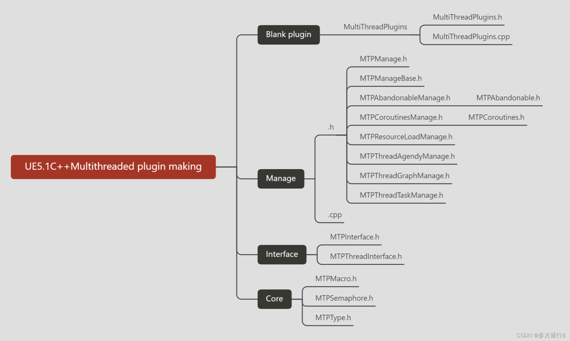
UE4/5C++多线程插件制作(0.简介)
目录 插件介绍 插件效果 插件使用 English 插件介绍 该插件制作,将从零开始,由一个空白插件一点点的制作,从写一个效果到封装,层层封装插件,简单粗暴的对插件进行了制作: 插件效果 更多的是在cpp中去…...
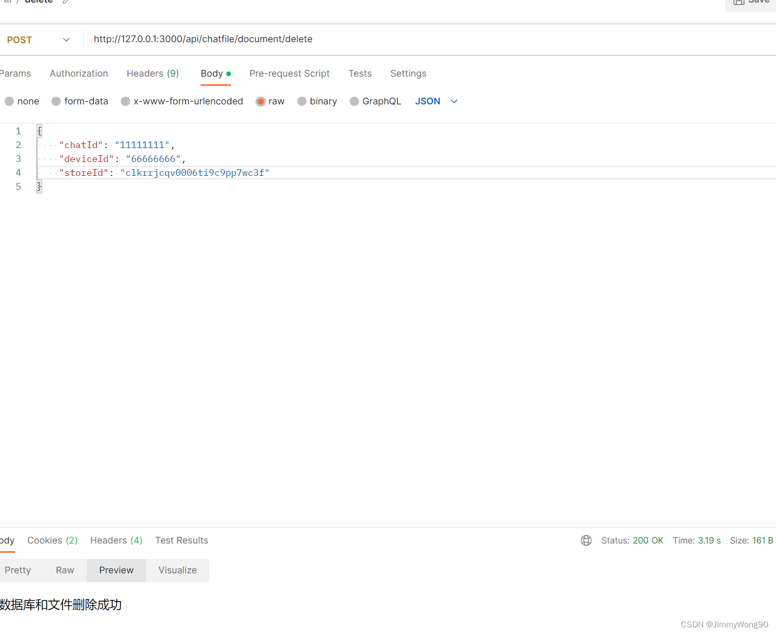
ChatFile实现相关流程
文本上传构建向量库后台库的内容 调用上传文件接口先上传文件 存在疑问:暂时是把文件保存在tmp文件夹,定时清理,是否使用云存储 根据不同的文件类型选取不同的文件加载器加载文件内容 switch (file.mimetype) {case application/pdf:loader new PDFLoader(file.path)breakc…...

15 文本编辑器vim
15.1 建立文件命令 如果file.txt就是修改这个文件,如果不存在就是新建一个文件。 vim file.txt 使用vim建完文件后,会自动进入文件中。 15.2 切换模式 底部要是显示插入,是编辑模式; 按esc,底部要是空白的࿰…...
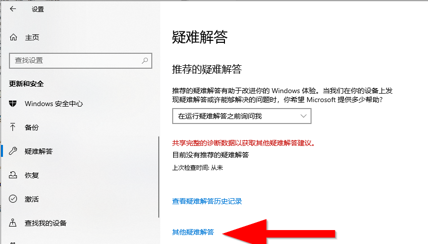
如何运行疑难解答程序来查找和修复Windows 10中的常见问题
如果Windows 10中出现问题,运行疑难解答可能会有所帮助。疑难解答人员可以为你找到并解决许多常见问题。 一、在控制面板中运行疑难解答 1、打开控制面板(图标视图),然后单击“疑难解答”图标。 2、单击“疑难解答”中左上角的…...
程序员成长之路心得篇——高效编码诀窍
随着AIGC的飞速发展,程序员越来越能够感受到外界和自己的压力。如何能够在AI蓬勃发展的时代不至于落后,不至于被替代?项目的开发效率起了至关重要的作用。 首先提出几个问题: 如何实现高效编程?高效编程的核心在于哪里ÿ…...
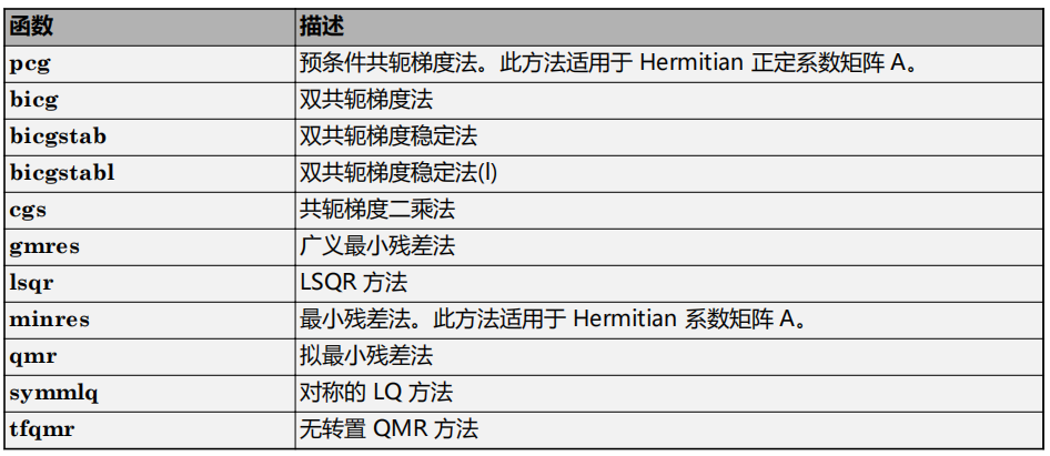
matlab使用教程(6)—线性方程组的求解
进行科学计算时,最重要的一个问题是对联立线性方程组求解。在矩阵表示法中,常见问题采用以下形式:给定两个矩阵 A 和 b,是否存在一个唯一矩阵 x 使 Ax b 或 xA b? 考虑一维示例具有指导意义。例如,方程 …...

Verilog语法学习——边沿检测
边沿检测 代码 module edge_detection_p(input sys_clk,input sys_rst_n,input signal_in,output edge_detected );//存储上一个时钟周期的输入信号reg signal_in_prev;always (posedge sys_clk or negedge sys_rst_n) beginif(!sys_rst_n)signal_in_prev < 0;else…...

springboot和springcloud的联系与区别
什么是springboot? Spring Boot是一个用于简化Spring应用程序开发的框架,它提供了一种约定优于配置的方式,通过自动配置和快速开发能力,可以快速搭建独立运行、生产级别的Spring应用程序。 在传统的Spring应用程序开发中…...

【Web开发指南】如何用MyEclipse进行JavaScript开发?
由于MyEclipse中有高级语法高亮显示、智能内容辅助和准确验证等特性,进行JavaScript编码不再是一项繁琐的任务。 MyEclipse v2023.1.2离线版下载 JavaScript项目 在MyEclipse 2021及以后的版本中,大多数JavaScript支持都是开箱即用的JavaScript源代码…...
【C++进阶】多态
⭐博客主页:️CS semi主页 ⭐欢迎关注:点赞收藏留言 ⭐系列专栏:C进阶 ⭐代码仓库:C进阶 家人们更新不易,你们的点赞和关注对我而言十分重要,友友们麻烦多多点赞+关注,你们的支持是我…...
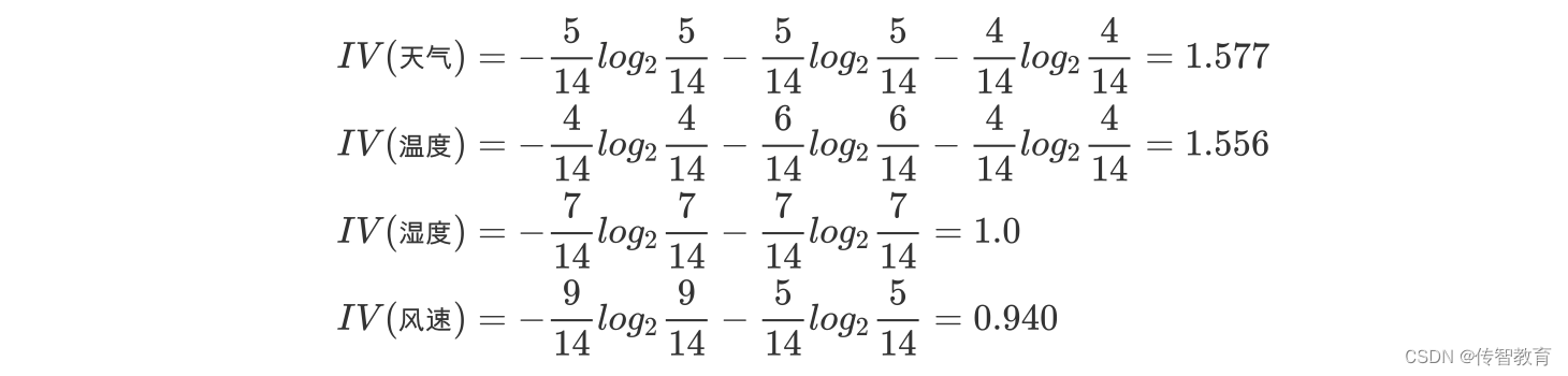
决策树的划分依据之:信息增益率
在上面的介绍中,我们有意忽略了"编号"这一列.若把"编号"也作为一个候选划分属性,则根据信息增益公式可计算出它的信息增益为 0.9182,远大于其他候选划分属性。 计算每个属性的信息熵过程中,我们发现,该属性的值为0, 也就…...

SolidUI社区-独立部署 和 Docker 通信分析
背景 随着文本生成图像的语言模型兴起,SolidUI想帮人们快速构建可视化工具,可视化内容包括2D,3D,3D场景,从而快速构三维数据演示场景。SolidUI 是一个创新的项目,旨在将自然语言处理(NLP)与计算机图形学相…...
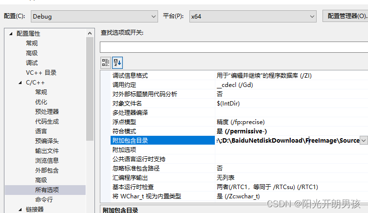
Windows下FreeImage库的配置
首先下载FreeImage库,http://freeimage.sourceforge.net/download.html,官网下载如下: 内部下载地址:https://download.csdn.net/download/qq_36314864/88140305 解压后,打开FreeImage.2017.sln,如果是vs…...

用python编写一个小程序,如何用python编写软件
大家好,给大家分享一下用python编写一个小程序,很多人还不知道这一点。下面详细解释一下。现在让我们来看看! 1、python可以写手机应用程序吗? 我想有人曲解意思了,人家说用python开发渣蔽一个手机app,不是…...

WPF实战学习笔记32-登录、注册服务添加
增加全局账户名同步 增加静态变量 添加文件:Mytodo.Common.Models.AppSession.cs ausing Prism.Mvvm; using System; using System.Collections.Generic; using System.ComponentModel; using System.Linq; using System.Text; using System.Threading.Tasks; us…...
XGBoost的参数
目录 1. 迭代过程 1.1 迭代次数/学习率/初始𝐻最大迭代值 1.1.1 参数num_boost_round & 参数eta 1.1.2 参数base_score 1.1.3 参数max_delta_step 1.2 xgboost的目标函数 1.2.1 gamma对模型的影响 1.2.2 lambda对模型的影响 2. XGBoost的弱评估器 2.…...

【已解决】windows7添加打印机报错:加载Tcp Mib库时的错误,无法加载标准TCP/IP端口的向导页
windows7 添加打印机的时候,输入完打印机的IP地址后,点击下一步,报错: 加载Tcp Mib库时的错误,无法加载标准TCP/IP端口的向导页 解决办法: 复制以下的代码到新建文本文档.txt中,然后修改文本文…...

年度名场面!黄仁勋逛胡同被投喂豆汁,眉头紧锁。网友:弥补了没有喝过 XX 的遗憾
5 月 15 日,「黄仁勋 南锣鼓巷」话题突然在多平台引爆热议。谁能想到,手握 5 万亿美刀市值的科技大佬,私下里竟是胡同干饭人。昨天在大会堂还是西装革履,今天老黄换上他的经典皮肤套装,带几名随行人员低调逛南锣鼓巷和…...

从ASCII到机器码:深入解析HEX文件的结构与校验机制
1. HEX文件的前世今生:从ASCII到机器码的桥梁 第一次接触HEX文件时,我也被那一串串看似毫无规律的十六进制字符搞得一头雾水。直到后来在嵌入式开发中频繁使用HEX文件进行固件升级,才真正理解了这个"翻译官"的重要性。HEX文件本质上…...

令牌管理实战:从JWT原理到token-ninja库的集成与应用
1. 项目概述:一个专为令牌处理而生的“忍者”如果你在开发中经常和令牌(Token)打交道,比如处理JWT、API密钥、会话标识,或者是在构建需要精细权限控制的微服务、身份认证系统,那你一定遇到过这些麻烦&#…...

轻量化目标检测实战:基于Pytorch的Mobilenet-YOLOv4融合架构设计与性能调优
1. 为什么需要轻量化目标检测模型 在移动端和嵌入式设备上运行目标检测模型时,我们常常面临两个关键挑战:计算资源有限和功耗约束。传统的YOLOv4虽然检测精度高,但其基于CSPDarknet53的主干网络参数量大、计算复杂度高,难以在资源…...

为什么你的民族志写作总卡在“分析乏力”?NotebookLM三步穿透文本深层文化逻辑
更多请点击: https://intelliparadigm.com 第一章:为什么你的民族志写作总卡在“分析乏力”?NotebookLM三步穿透文本深层文化逻辑 民族志写作常陷入“描述丰富、解释单薄”的困境——田野笔记堆叠如山,却难以提炼出文化实践背后的…...

Kubernetes Pod安全标准:构建零信任的容器运行环境
Kubernetes Pod安全标准:构建零信任的容器运行环境 一、Pod安全标准的核心概念与演进 1.1 容器安全的演进历程 容器技术的普及带来了部署效率的革命性提升,但同时也引入了新的安全挑战。从Docker早期的容器逃逸漏洞到Kubernetes集群的大规模安全事件&…...

明日方舟素材库:从游戏资产到创意引擎的技术解密
明日方舟素材库:从游戏资产到创意引擎的技术解密 【免费下载链接】ArknightsGameResource 明日方舟客户端素材 项目地址: https://gitcode.com/gh_mirrors/ar/ArknightsGameResource 在数字创作的广阔天地中,专业级游戏素材往往被锁在商业游戏的围…...

如何3步永久保存QQ空间十年回忆:GetQzonehistory数据备份实战指南
如何3步永久保存QQ空间十年回忆:GetQzonehistory数据备份实战指南 【免费下载链接】GetQzonehistory 获取QQ空间发布的历史说说 项目地址: https://gitcode.com/GitHub_Trending/ge/GetQzonehistory 在数字记忆时代,QQ空间承载了无数人的青春印记…...

ACID [Atomicity, Consistency, Isolation, Durability]
ACID [Atomicity, Consistency, Isolation, Durability] 原子性、一致性、隔离性、持久性package further.zwf.acid;import java.sql.Connection; import java.sql.DriverManager; import java.sql.PreparedStatement; import java.sql.SQLException;/*** MySQL 事务示例&am…...
:make与makefile)
第9课:Linux开发工具(四):make与makefile
第9课:Linux开发工具(四):make与makefile 一、为什么我们需要 Makefile? 1.1 IDE 背后的秘密 在使用 Visual Studio 等 IDE 时,我们只需按下 F5 或点击"编译"按钮,程序就会自动完成编…...