《视觉 SLAM 十四讲》V2 第 4 讲 李群与李代数 【什么样的相机位姿 最符合 当前观测数据】
P71
文章目录
- 4.1 李群与李代数基础
- 4.1.3 李代数的定义
- 4.1.4 李代数 so(3)
- 4.1.5 李代数 se(3)
- 4.2 指数与对数映射
- 4.2.1 SO(3)上的指数映射
- 罗德里格斯公式推导
- 4.2.2 SE(3) 上的指数映射
- SO(3),SE(3),so(3),se(3)的对应关系
- 4.3 李代数求导与扰动模型
- 4.3.2 SO(3)上的李代数求导
- 4.3.3 李代数求导
- 4.3.4 扰动模型(左乘)【更简单 的导数计算模型】
- 4.3.5 SE(3)上的李代数求导
- 4.4 Sophus应用 【Code】
- 4.4.2 评估轨迹的误差 【Code】
- 4.5 相似变换群 与 李代数
- 习题
- 题1
- 题2
- 题4
- √ 题5
- √ 题6
- 6.2 SE(3)伴随性质
- √ 题7
- √ 题8
- LaTex

什么样的相机位姿 最符合 当前观测数据。
求解最优的 R , t \bm{R, t} R,t, 使得误差最小化。
4.1 李群与李代数基础

群: 只有一个(良好的)运算的集合。

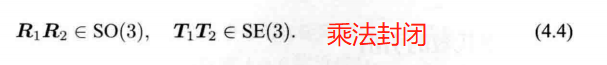

封结幺逆 、 丰俭由你

李群: 具有连续(光滑)性质的群。


在 t = 0 附近,旋转矩阵可以由 e x p ( ϕ 0 ˆ t ) exp(\phi_0\^{}t) exp(ϕ0ˆt)计算得到
4.1.3 李代数的定义

李代数 描述了李群的局部性质
- 单位元 附近的正切空间。
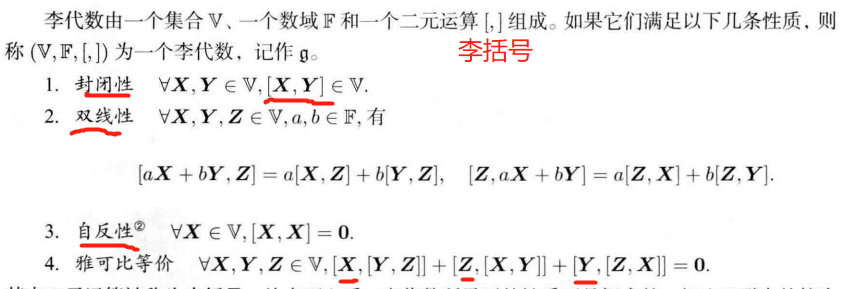
g = ( R 3 , R , × ) \mathfrak{g}=(\mathbb{R}^3, \mathbb{R}, \times) g=(R3,R,×)构成了一个李代数
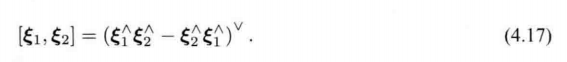
4.1.4 李代数 so(3)
s o ( 3 ) \mathfrak{so}(3) so(3): 一个由三维向量组成的集合,每个向量对应一个反对称矩阵,可以用于表达旋转矩阵的导数。
s o ( 3 ) = { ϕ ∈ R 3 , Φ = ϕ ˆ ∈ R 3 × 3 } \mathfrak{so}(3)=\{\phi\in\mathbb{R}^3,\bm{\Phi}=\phi\^{}\in\mathbb{R}^{3\times3}\} so(3)={ϕ∈R3,Φ=ϕˆ∈R3×3}


4.1.5 李代数 se(3)
李群 S E ( 3 ) SE(3) SE(3) 对应的李代数 s e ( 3 ) \mathfrak{se}(3) se(3)


4.2 指数与对数映射
4.2.1 SO(3)上的指数映射
s o ( 3 ) \mathfrak{so}(3) so(3): 旋转向量 组成的空间
指数映射: 罗德里格斯公式
R = e x p ( ϕ ∧ ) = e x p ( θ a ∧ ) = c o s θ I + ( 1 − c o s θ ) a a T + s i n θ a ∧ \bm{R}=exp(\phi^{\land})=exp(\theta\bm{a}^{\land})=cos\theta\bm{I} + (1-cos\theta)\bm{a}\bm{a}^T+sin\theta\bm{a}^{\land} R=exp(ϕ∧)=exp(θa∧)=cosθI+(1−cosθ)aaT+sinθa∧
对数映射: 李群 S O ( 3 ) SO(3) SO(3) 中的元素 ——> 李代数 s o ( 3 ) \mathfrak{so}(3) so(3)

把旋转角固定在 ± π ±\pi ±π 之间,则李群和李代数 元素 一一对应。
————————————————
罗德里格斯公式推导
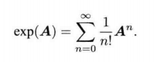

e x p ( ϕ ∧ ) = e x p ( θ a ∧ ) = ∑ n = 0 ∞ 1 n ! ( θ a ∧ ) n n = 0 , 1 , 2 , 3 , . . . 原式 = I + θ a ∧ + 1 2 ! θ 2 a ∧ a ∧ + 1 3 ! θ 3 a ∧ a ∧ a ∧ + 1 4 ! θ 4 ( a ∧ ) 4 + ⋅ ⋅ ⋅ 将 a ∧ a ∧ = a a T − I ; a ∧ a ∧ a ∧ = ( a ∧ ) 3 = − a ∧ 代入 原式 = a a T − a ∧ a ∧ + θ a ∧ + 1 2 ! θ 2 a ∧ a ∧ − 1 3 ! θ 3 a ∧ − 1 4 ! θ 4 ( a ∧ ) 2 + ⋅ ⋅ ⋅ = a a T + ( θ − 1 3 ! θ 3 + 1 5 ! θ 5 − ⋅ ⋅ ⋅ ) a ∧ − ( 1 − 1 2 ! θ 2 + 1 4 ! θ 4 − ⋅ ⋅ ⋅ ) a ∧ a ∧ = a ∧ a ∧ + I + s i n θ a ∧ − c o s θ a ∧ a ∧ = ( 1 − c o s θ ) a ∧ a ∧ + I + s i n θ a ∧ = ( 1 − c o s θ ) ( a a T − I ) + I + s i n θ a ∧ = c o s θ I + ( 1 − c o s θ ) a a T + s i n θ a ∧ \begin{align*}exp(\phi^{\land}) &=exp(\theta\bm{a}^{\land})=\sum\limits_{n=0}^{\infty}\frac{1}{n!} (\theta\bm{a}^{\land})^n \\ & n = 0, 1, 2, 3, ... \\ 原式 & = \bm{I} + \theta\bm{a}^{\land} + \frac{1}{2!}\theta^2\bm{a}^{\land}\bm{a}^{\land} + \frac{1}{3!}\theta^3\bm{a}^{\land}\bm{a}^{\land}\bm{a}^{\land} +\frac{1}{4!}\theta^4(\bm{a}^{\land})^4+···\\ & 将\bm{a}^{\land}\bm{a}^{\land} = \bm{a}\bm{a}^T - \bm{I}; \bm{a}^{\land}\bm{a}^{\land}\bm{a}^{\land} = (\bm{a}^{\land})^3 =-\bm{a}^{\land} 代入 \\ 原式& = \bm{a}\bm{a}^T - \bm{a}^{\land}\bm{a}^{\land} + \theta\bm{a}^{\land} + \frac{1}{2!}\theta^2\bm{a}^{\land}\bm{a}^{\land}-\frac{1}{3!}\theta^3\bm{a}^{\land}-\frac{1}{4!}\theta^4(\bm{a}^{\land})^2+···\\ & = \bm{a}\bm{a}^T + (\theta - \frac{1}{3!}\theta^3+\frac{1}{5!}\theta^5-···)\bm{a}^{\land}-(1-\frac{1}{2!}\theta^2+\frac{1}{4!}\theta^4-···)\bm{a}^{\land}\bm{a}^{\land}\\ & = \bm{a}^{\land}\bm{a}^{\land} + \bm{I}+sin\theta \bm{a}^{\land}-cos\theta\bm{a}^{\land}\bm{a}^{\land}\\ &=(1-cos\theta)\bm{a}^{\land}\bm{a}^{\land}+\bm{I} + sin\theta\bm{a}^{\land}\\ &= (1-cos\theta)(\bm{a}\bm{a}^T-\bm{I})+\bm{I} + sin\theta\bm{a}^{\land}\\ & = cos\theta\bm{I}+ (1-cos\theta)\bm{a}\bm{a}^T + sin\theta\bm{a}^{\land} \end{align*} exp(ϕ∧)原式原式=exp(θa∧)=n=0∑∞n!1(θa∧)nn=0,1,2,3,...=I+θa∧+2!1θ2a∧a∧+3!1θ3a∧a∧a∧+4!1θ4(a∧)4+⋅⋅⋅将a∧a∧=aaT−I;a∧a∧a∧=(a∧)3=−a∧代入=aaT−a∧a∧+θa∧+2!1θ2a∧a∧−3!1θ3a∧−4!1θ4(a∧)2+⋅⋅⋅=aaT+(θ−3!1θ3+5!1θ5−⋅⋅⋅)a∧−(1−2!1θ2+4!1θ4−⋅⋅⋅)a∧a∧=a∧a∧+I+sinθa∧−cosθa∧a∧=(1−cosθ)a∧a∧+I+sinθa∧=(1−cosθ)(aaT−I)+I+sinθa∧=cosθI+(1−cosθ)aaT+sinθa∧
e x p ( θ a ∧ ) = c o s θ I + ( 1 − c o s θ ) a a T + s i n θ a ∧ exp(\theta\bm{a}^{\land})=cos\theta\bm{I} + (1-cos\theta)\bm{a}\bm{a}^T+sin\theta\bm{a}^{\land} exp(θa∧)=cosθI+(1−cosθ)aaT+sinθa∧
—————

$\bm{a}^{\land}$
a ∧ \bm{a}^{\land} a∧
————————————————
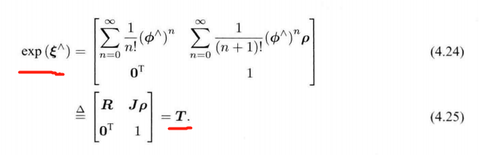
4.2.2 SE(3) 上的指数映射
——————
推导:
∑ n = 0 ∞ 1 ( n + 1 ) ! ( ϕ ∧ ) n = ∑ n = 0 ∞ 1 ( n + 1 ) ! ( θ a ∧ ) n = I + 1 2 ! θ a ∧ + 1 3 ! θ 2 ( a ∧ ) 2 + 1 4 ! θ 3 ( a ∧ ) 3 + 1 5 ! θ 4 ( a ∧ ) 4 + ⋅ ⋅ ⋅ = 1 θ ( 1 2 ! θ 2 − 1 4 ! θ 4 + ⋅ ⋅ ⋅ ) a ∧ + 1 θ ( 1 3 ! θ 3 − 1 5 ! θ 5 + ⋅ ⋅ ⋅ ) ( a ∧ ) 2 + I = 1 θ ( 1 − c o s θ ) a ∧ + 1 θ ( θ − s i n θ ) ( a a T − I ) + I = s i n θ θ I + ( 1 − s i n θ θ ) a a T + 1 − c o s θ θ a ∧ = d e f J \begin{align*} \sum\limits_{n=0}^{\infty}\frac{1}{(n+1)!}(\phi^{\land})^n &= \sum\limits_{n=0}^{\infty}\frac{1}{(n+1)!}(\theta\bm{a}^{\land})^n\\ & = \bm{I} + \frac{1}{2!}\theta\bm{a}^{\land} + \frac{1}{3!}\theta^2(\bm{a}^{\land})^2 + \frac{1}{4!}\theta^3(\bm{a}^{\land})^3 + \frac{1}{5!}\theta^4(\bm{a}^{\land})^4+···\\ & = \frac{1}{\theta}( \frac{1}{2!}\theta^2- \frac{1}{4!}\theta^4+···)\bm{a}^{\land} + \frac{1}{\theta}( \frac{1}{3!}\theta^3- \frac{1}{5!}\theta^5+···)(\bm{a}^{\land})^2+\bm{I} \\ & = \frac{1}{\theta}( 1-cos\theta)\bm{a}^{\land} + \frac{1}{\theta}(\theta-sin\theta)(\bm{a}\bm{a}^T-\bm{I})+\bm{I} \\ & = \frac{sin\theta}{\theta}\bm{I}+(1-\frac{sin\theta}{\theta})\bm{a}\bm{a}^T + \frac{1-cos\theta}{\theta}\bm{a}^{\land}\\ & \overset{\mathrm{def}}{=} \bm{J} \end{align*} n=0∑∞(n+1)!1(ϕ∧)n=n=0∑∞(n+1)!1(θa∧)n=I+2!1θa∧+3!1θ2(a∧)2+4!1θ3(a∧)3+5!1θ4(a∧)4+⋅⋅⋅=θ1(2!1θ2−4!1θ4+⋅⋅⋅)a∧+θ1(3!1θ3−5!1θ5+⋅⋅⋅)(a∧)2+I=θ1(1−cosθ)a∧+θ1(θ−sinθ)(aaT−I)+I=θsinθI+(1−θsinθ)aaT+θ1−cosθa∧=defJ
J = s i n θ θ I + ( 1 − s i n θ θ ) a a T + 1 − c o s θ θ a ∧ \bm{J}=\frac{sin\theta}{\theta}\bm{I}+(1-\frac{sin\theta}{\theta})\bm{a}\bm{a}^T + \frac{1-cos\theta}{\theta}\bm{a}^{\land} J=θsinθI+(1−θsinθ)aaT+θ1−cosθa∧
R = c o s θ I + ( 1 − c o s θ ) a a T + s i n θ a ∧ \bm{R}=cos\theta\bm{I}+(1-cos\theta)\bm{a}\bm{a}^T + sin\theta\bm{a}^{\land} R=cosθI+(1−cosθ)aaT+sinθa∧
————
t = J ρ \bm{t=Jρ} t=Jρ
平移部分发生了一次以 J \bm{J} J 为系数矩阵的 线性变换。
SO(3),SE(3),so(3),se(3)的对应关系

4.3 李代数求导与扰动模型
Baker-Campbell-Hausdorff公式(BCH公式)


4.3.2 SO(3)上的李代数求导
位姿由SO(3)上的旋转矩阵 或 SE(3)上的变换矩阵 描述
设某时刻机器人的位姿为 T \bm{T} T, 观察到了一个世界坐标位于 p \bm{p} p 的点,产生了一个观测数据 z \bm{z} z
计算理想的观测与实际数据之间的误差: e = z − T p \bm{e = z-Tp} e=z−Tp
假设一共有 N N N 个这样的路标点和观测,对机器人进行位姿估计,相当于寻找一个最优的 T \bm{T} T ,使得整体误差最小化:
min T J ( T ) = ∑ i = 1 N ∣ ∣ z i − T p i ∣ ∣ 2 2 \min\limits_{\bm{T}}J(\bm{T}) = \sum\limits_{i=1}^{N}||\bm{z_i-Tp_i}||_2^2 TminJ(T)=i=1∑N∣∣zi−Tpi∣∣22
求解上述问题,需要计算目标函数 J J J 关于变换矩阵 T \bm{T} T 的导数。
使用 李代数 解决 求导问题 的2种思路:
1、用李代数表示姿态,然后根据李代数加法对李代数求导。
2、对李群左乘或右乘微小扰动,然后对该扰动求导,称为左扰动和右扰动模型。
4.3.3 李代数求导

——————
推导:
∂ ( R p ) ∂ R = R 对应的李代数为 ϕ ∂ ( exp ( ϕ ∧ ) p ) ∂ ϕ = lim Δ ϕ → 0 exp ( ( ϕ + Δ ϕ ) ∧ ) p − exp ( ϕ ∧ ) p Δ ϕ 由式 ( 4.35 ) = lim Δ ϕ → 0 exp ( ( J l Δ ϕ ) ∧ ) exp ( ϕ ∧ ) p − exp ( ϕ ∧ ) p Δ ϕ = lim Δ ϕ → 0 ( I + ( J l Δ ϕ ) ∧ ) exp ( ϕ ∧ ) p − exp ( ϕ ∧ ) p Δ ϕ = lim Δ ϕ → 0 ( J l Δ ϕ ) ∧ exp ( ϕ ∧ ) p Δ ϕ a ∧ 等效于 a × , 因此根据叉乘的性质 = lim Δ ϕ → 0 − ( exp ( ϕ ∧ ) p ) ∧ J l Δ ϕ Δ ϕ = − ( R p ) ∧ J l \begin{align*}\frac{\partial(\bm{Rp})}{\partial\bm{R}} &\xlongequal{R对应的李代数为\phi}\frac{\partial(\exp(\phi^{\land})\bm{p})}{\partial\phi} \\ & = \lim\limits_{Δ\phi\to0}\frac{\exp((\phi+Δ\phi)^{\land})\bm{p}-\exp(\phi^{\land})\bm{p}}{Δ\phi} \\ & 由 式(4.35)\\ & = \lim\limits_{Δ\phi\to0}\frac{\exp((\bm{J}_lΔ\phi)^{\land})\exp(\phi^{\land})\bm{p}-\exp(\phi^{\land})\bm{p}}{Δ\phi} \\ & = \lim\limits_{Δ\phi\to0}\frac{(\bm{I}+(\bm{J}_lΔ\phi)^{\land})\exp(\phi^{\land})\bm{p}-\exp(\phi^{\land})\bm{p}}{Δ\phi} \\ & = \lim\limits_{Δ\phi\to0}\frac{(\bm{J}_lΔ\phi)^{\land}\exp(\phi^{\land})\bm{p}}{Δ\phi} \\ & a^{\land} 等效于 a \times ,因此根据叉乘的性质 \\ & = \lim\limits_{Δ\phi\to0}\frac{-(\exp(\phi^{\land})\bm{p})^{\land}\bm{J}_lΔ\phi}{Δ\phi} \\ & = -(\bm{Rp})^{\land}\bm{J}_l \end{align*} ∂R∂(Rp)R对应的李代数为ϕ∂ϕ∂(exp(ϕ∧)p)=Δϕ→0limΔϕexp((ϕ+Δϕ)∧)p−exp(ϕ∧)p由式(4.35)=Δϕ→0limΔϕexp((JlΔϕ)∧)exp(ϕ∧)p−exp(ϕ∧)p=Δϕ→0limΔϕ(I+(JlΔϕ)∧)exp(ϕ∧)p−exp(ϕ∧)p=Δϕ→0limΔϕ(JlΔϕ)∧exp(ϕ∧)pa∧等效于a×,因此根据叉乘的性质=Δϕ→0limΔϕ−(exp(ϕ∧)p)∧JlΔϕ=−(Rp)∧Jl
∂ ( exp ( ϕ ∧ ) p ) ∂ ϕ = − ( R p ) ∧ J l \frac{\partial(\exp(\phi^{\land})\bm{p})}{\partial\phi} = -(\bm{Rp})^{\land}\bm{J}_l ∂ϕ∂(exp(ϕ∧)p)=−(Rp)∧Jl
——————
4.3.4 扰动模型(左乘)【更简单 的导数计算模型】
对 R \bm{R} R 进行一次扰动 Δ R Δ\bm{R} ΔR ,看结果对于 扰动的变化率。
设左扰动 Δ R Δ\bm{R} ΔR 对应的李代数 为 φ \varphi φ
∂ ( R p ) ∂ φ = lim φ → 0 exp ( φ ∧ ) exp ( ϕ ∧ ) p − exp ( ϕ ∧ ) p φ = lim φ → 0 ( I + φ ∧ ) exp ( ϕ ∧ ) p − exp ( ϕ ∧ ) p φ = lim φ → 0 φ ∧ exp ( ϕ ∧ ) p φ = lim φ → 0 φ ∧ R p φ = lim φ → 0 − ( R p ) ∧ φ φ = − ( R p ) ∧ \begin{align*}\frac{\partial(\bm{Rp})}{\partial\varphi} &= \lim\limits_{\varphi\to0}\frac{\exp(\varphi^{\land})\exp(\phi^{\land})\bm{p}-\exp(\phi^{\land})\bm{p}}{\varphi}\\ &= \lim\limits_{\varphi\to0}\frac{(\bm{I} + \varphi^{\land})\exp(\phi^{\land})\bm{p}-\exp(\phi^{\land})\bm{p}}{\varphi}\\ &= \lim\limits_{\varphi\to0}\frac{\varphi^{\land}\exp(\phi^{\land})\bm{p}}{\varphi}\\ &= \lim\limits_{\varphi\to0}\frac{\varphi^{\land}\bm{Rp}}{\varphi}\\ &= \lim\limits_{\varphi\to0}\frac{-(\bm{Rp})^{\land}\varphi}{\varphi}\\ &= -(\bm{Rp})^{\land} \end{align*} ∂φ∂(Rp)=φ→0limφexp(φ∧)exp(ϕ∧)p−exp(ϕ∧)p=φ→0limφ(I+φ∧)exp(ϕ∧)p−exp(ϕ∧)p=φ→0limφφ∧exp(ϕ∧)p=φ→0limφφ∧Rp=φ→0limφ−(Rp)∧φ=−(Rp)∧
4.3.5 SE(3)上的李代数求导
假设某空间点 p \bm{p} p 经过一次变换 T \bm{T} T (对应李代数为 ξ \bm{\xi} ξ), 得到 T p \bm{Tp} Tp
现在给 T \bm{T} T 左乘一个扰动 Δ T = exp ( Δ ξ ∧ ) Δ\bm{T} = \exp(Δ\bm{\xi}^{\land}) ΔT=exp(Δξ∧)
设扰动项的李代数为 Δ ξ = [ Δ ρ , Δ ϕ ] T Δ\bm{\xi}=[Δ\bm{\rho},Δ\bm{\phi}]^T Δξ=[Δρ,Δϕ]T,则

∂ ( T p ) ∂ Δ ξ = lim Δ ξ → 0 exp ( Δ ξ ∧ ) exp ( ξ ∧ ) p − exp ( ξ ∧ ) p Δ ξ = lim Δ ξ → 0 ( I + Δ ξ ∧ ) exp ( ξ ∧ ) p − exp ( ξ ∧ ) p Δ ξ = lim Δ ξ → 0 Δ ξ ∧ exp ( ξ ∧ ) p Δ ξ = lim Δ ξ → 0 [ Δ ϕ ∧ Δ ρ 0 T 0 ] [ R p + t 1 ] Δ ξ = lim Δ ξ → 0 [ Δ ϕ ∧ ( R p + t ) + Δ ρ 0 T ] [ Δ ρ , Δ ϕ ] T = [ I − ( R p + t ) ∧ 0 T 0 T ] = d e f ( T p ) ⨀ \begin{align*}\frac{\partial(\bm{Tp})}{\partial{Δ\bm{\xi}}} &= \lim\limits_{Δ\bm{\xi}\to0}\frac{\exp(Δ\bm{\xi}^{\land})\exp(\bm{\xi}^{\land})\bm{p}-\exp(\bm{\xi}^{\land})\bm{p}}{Δ\bm{\xi}} \\ &= \lim\limits_{Δ\bm{\xi}\to0}\frac{(\bm{I} +Δ\bm{\xi}^{\land})\exp(\bm{\xi}^{\land})\bm{p}-\exp(\bm{\xi}^{\land})\bm{p}}{Δ\bm{\xi}} \\ &= \lim\limits_{Δ\bm{\xi}\to0}\frac{Δ\bm{\xi}^{\land}\exp(\bm{\xi}^{\land})\bm{p}}{Δ\bm{\xi}} \\ &=\lim\limits_{Δ\bm{\xi}\to0} \frac{\begin{bmatrix} Δ\bm{\phi}^{\land} & \Delta\bm{\rho}\\ \bm{0}^T & 0 \end{bmatrix}\begin{bmatrix} \bm{Rp+t}\\ 1 \end{bmatrix}}{Δ\bm{\xi}}\\ &=\lim\limits_{Δ\bm{\xi}\to0} \frac{\begin{bmatrix} \Delta\bm{\phi}^{\land}(\bm{Rp+t})+\Delta\bm{\rho}\\ \bm{0}^T \end{bmatrix}}{[Δ\bm{\rho},Δ\bm{\phi}]^T} \\ & = \begin{bmatrix} \bm{I} & -(\bm{Rp+t})^{\land} \\ \bm{0}^T & \bm{0}^T \end{bmatrix} \\ &\overset{\mathrm{def}}{=}(\bm{Tp})^{\bigodot} \end{align*} ∂Δξ∂(Tp)=Δξ→0limΔξexp(Δξ∧)exp(ξ∧)p−exp(ξ∧)p=Δξ→0limΔξ(I+Δξ∧)exp(ξ∧)p−exp(ξ∧)p=Δξ→0limΔξΔξ∧exp(ξ∧)p=Δξ→0limΔξ[Δϕ∧0TΔρ0][Rp+t1]=Δξ→0lim[Δρ,Δϕ]T[Δϕ∧(Rp+t)+Δρ0T]=[I0T−(Rp+t)∧0T]=def(Tp)⨀

$\overset{\mathrm{def}}{=}(\bm{Tp})^{\bigodot}$
4.4 Sophus应用 【Code】
SO(3)、SE(3)
二维运动SO(2)和SE(2)
相似变换 Sim(3)
mkdir build && cd build
cmake ..
make
./useSophus
CMakeLists.txt
cmake_minimum_required(VERSION 2.8)project(useSophus)find_package(Sophus REQUIRED)
include_directories( ${Sophus_INCLUDE_DIRS})add_executable(useSophus useSophus.cpp)
target_link_libraries(useSophus ${Sophus_LIBRARIES})
#include<iostream>
#include<cmath>
#include<Eigen/Core>
#include<Eigen/Geometry>
#include "sophus/se3.h"using namespace std;
using namespace Eigen;/* sophus 的基本用法 */
int main(int argc, char **argv){// 沿 Z轴  转90° 的旋转矩阵Matrix3d R = AngleAxisd(M_PI/2, Vector3d(0, 0, 1)).toRotationMatrix();/* 四元数 */Quaterniond q(R);Sophus::SO3 SO3_R(R);Sophus::SO3 SO3_q(q);cout << "SO(3) from matrix:\n" << SO3_R.matrix() << endl;cout << "SO(3) from quatenion:\n" << SO3_q.matrix() << endl;cout << "they are equal" << endl;return 0;
}

#include<iostream>
#include<cmath>
#include<Eigen/Core>
#include<Eigen/Geometry>
#include "sophus/se3.h"using namespace std;
using namespace Eigen;/* sophus 的基本用法 */
int main(int argc, char **argv){/* 使用 对数映射 获得  李代数*/Matrix3d R = AngleAxisd(M_PI/2, Vector3d(0, 0, 1)).toRotationMatrix();Sophus::SO3 SO3_R(R);Vector3d so3 = SO3_R.log();cout << "so3 = " << so3.transpose() << endl;// hat  向量 ——> 反对称矩阵cout << "so3 hat = \n" << Sophus::SO3::hat(so3)<< endl;// vee  反对称 ——> 向量cout << "so3 hat vee = " << Sophus::SO3::vee(Sophus::SO3::hat(so3)).transpose() << endl;Vector3d update_so3(1e-4, 0, 0);// 假设更新量为这么多Sophus::SO3 SO3_updated =Sophus::SO3::exp(update_so3) * SO3_R;cout << "SO3 updated = \n" << SO3_updated.matrix() << endl;return 0;
}

#include<iostream>
#include<cmath>
#include<Eigen/Core>
#include<Eigen/Geometry>
#include "sophus/se3.h"using namespace std;
using namespace Eigen;/* sophus   SE(3) 的基本用法 */
int main(int argc, char **argv){Matrix3d R = AngleAxisd(M_PI/2, Vector3d(0, 0, 1)).toRotationMatrix();  // 沿 Z轴 旋转 90° 的旋转矩阵Vector3d t(1, 0, 0);  // 沿 X 轴平移1Sophus::SE3 SE3_Rt(R, t);  // 从R,t 构造 SE(3)Quaterniond q(R);Sophus::SE3 SE3_qt(q, t); // 从q, t 构造 SE(3)cout << "SE3 from R, t = \n" << SE3_Rt.matrix() << endl;cout << "SE3 from q, t = \n" << SE3_qt.matrix() << endl; /* 李代数se(3) 是一个 6 维 向量*/typedef Eigen::Matrix<double, 6, 1> Vector6d;Vector6d se3 = SE3_Rt.log();cout << "se3 = " << se3.transpose() << endl;// hat  向量 ——> 反对称矩阵cout << "se3 hat = \n" << Sophus::SE3::hat(se3)<< endl;// vee  反对称 ——> 向量cout << "se3 hat vee = " << Sophus::SE3::vee(Sophus::SE3::hat(se3)).transpose() << endl;// 更新Vector6d update_se3;// 更新量update_se3.setZero();update_se3(0, 0) = 1e-4;Sophus::SE3 SE3_updated =Sophus::SE3::exp(update_se3) * SE3_Rt;cout << "SE3 updated = \n" << SE3_updated.matrix() << endl;return 0;
}

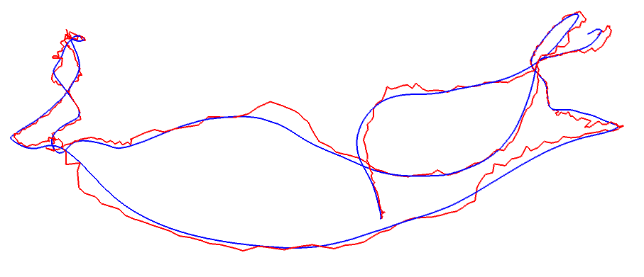
4.4.2 评估轨迹的误差 【Code】
————————
考虑一条估计轨迹 T e s t i , i \bm{T}_{esti,i} Testi,i 和真实轨迹 T g t , i \bm{T}_{gt,i} Tgt,i ,其中 i = 1 , ⋅ ⋅ ⋅ , N i= 1,···,N i=1,⋅⋅⋅,N
1、绝对误差轨迹(Absolute Trajectory Error, ATE) 旋转和平移误差
A T E a l l = 1 N ∑ i = 1 N ∣ ∣ l o g ( T g t , i − 1 T e s t i , i ) ∨ ∣ ∣ 2 2 ATE_{all}=\sqrt{\frac{1}{N}\sum\limits_{i=1}^{N}||log(\bm{T}_{gt,i}^{-1}\bm{T}_{esti,i})^{\vee}||_2^2} ATEall=N1i=1∑N∣∣log(Tgt,i−1Testi,i)∨∣∣22
- 每个位姿 李代数 的均方根误差 (Root-Mean-Squared Error,RMSE)
2、绝对平移误差(Average Translational Error)
A T E t r a n s = 1 N ∑ i = 1 N ∣ ∣ t r a n s ( T g t , i − 1 T e s t i , i ) ∣ ∣ 2 2 ATE_{trans}=\sqrt{\frac{1}{N}\sum\limits_{i=1}^{N}||trans(\bm{T}_{gt,i}^{-1}\bm{T}_{esti,i})||_2^2} ATEtrans=N1i=1∑N∣∣trans(Tgt,i−1Testi,i)∣∣22
其中 trans 表示 取括号内部变量的平移部分。
- 从整条轨迹上看,旋转出现偏差后,随后的轨迹在平移上也会出现误差。
3、相对误差
考虑 i i i 时刻到 i + Δ t i+\Delta t i+Δt 的运动,相对位姿误差(Relative Pose Error, RPE)
R P E a l l = 1 N − Δ t ∑ i = 1 N − Δ t ∣ ∣ l o g ( ( T g t , i − 1 T g t , i + Δ t ) − 1 ( T e s t i , i − 1 T e s t i , i + Δ t ) ) ∨ ∣ ∣ 2 2 RPE_{all}=\sqrt{\frac{1}{N-\Delta t}\sum\limits_{i=1}^{N-\Delta t}||log((\bm{T}_{gt,i}^{-1}\bm{T}_{gt,i+\Delta t})^{-1}(\bm{T}_{esti,i}^{-1}\bm{T}_{esti,i+\Delta t}))^{\vee}||_2^2} RPEall=N−Δt1i=1∑N−Δt∣∣log((Tgt,i−1Tgt,i+Δt)−1(Testi,i−1Testi,i+Δt))∨∣∣22
R P E t r a n s = 1 N − Δ t ∑ i = 1 N − Δ t ∣ ∣ t r a n s ( ( T g t , i − 1 T g t , i + Δ t ) − 1 ( T e s t i , i − 1 T e s t i , i + Δ t ) ) ∣ ∣ 2 2 RPE_{trans}=\sqrt{\frac{1}{N-\Delta t}\sum\limits_{i=1}^{N-\Delta t}||trans((\bm{T}_{gt,i}^{-1}\bm{T}_{gt,i+\Delta t})^{-1}(\bm{T}_{esti,i}^{-1}\bm{T}_{esti,i+\Delta t}))||_2^2} RPEtrans=N−Δt1i=1∑N−Δt∣∣trans((Tgt,i−1Tgt,i+Δt)−1(Testi,i−1Testi,i+Δt))∣∣22
————————

mkdir build && cd build
cmake ..
make
./trajectoryError
CMakeLists.txt
cmake_minimum_required(VERSION 2.8)project(trajectoryError)find_package(Sophus REQUIRED)
include_directories( ${Sophus_INCLUDE_DIRS})option(USE_UBUNTU_20 "Set to ON if you are using Ubuntu 20.04" OFF)
find_package(Pangolin REQUIRED)
if(USE_UBUNTU_20)message("You are using Ubuntu 20.04, fmt::fmt will be linked")find_package(fmt REQUIRED)set(FMT_LIBRARIES fmt::fmt)
endif()
include_directories(${Pangolin_INCLUDE_DIRS})add_executable(trajectoryError trajectoryError.cpp)
target_link_libraries(trajectoryError ${Sophus_LIBRARIES})
target_link_libraries(trajectoryError ${Pangolin_LIBRARIES} ${FMT_LIBRARIES})
trajectoryError.cpp
#include <iostream>
#include <fstream>
#include <unistd.h>
#include <pangolin/pangolin.h>
#include <sophus/se3.h>using namespace Sophus;
using namespace std;string groundtruth_file = "../groundtruth.txt";
string estimated_file = "../estimated.txt";typedef vector<Sophus::SE3, Eigen::aligned_allocator<Sophus::SE3>> TrajectoryType;void DrawTrajectory(const TrajectoryType >, const TrajectoryType &esti);TrajectoryType ReadTrajectory(const string &path);int main(int argc, char **argv) {TrajectoryType groundtruth = ReadTrajectory(groundtruth_file);TrajectoryType estimated = ReadTrajectory(estimated_file);assert(!groundtruth.empty() && !estimated.empty());assert(groundtruth.size() == estimated.size());// compute rmsedouble rmse = 0;for (size_t i = 0; i < estimated.size(); i++) {Sophus::SE3 p1 = estimated[i], p2 = groundtruth[i];double error = (p2.inverse() * p1).log().norm();rmse += error * error;}rmse = rmse / double(estimated.size());rmse = sqrt(rmse);cout << "RMSE = " << rmse << endl;DrawTrajectory(groundtruth, estimated);return 0;
}TrajectoryType ReadTrajectory(const string &path) {ifstream fin(path);TrajectoryType trajectory;if (!fin) {cerr << "trajectory " << path << " not found." << endl;return trajectory;}while (!fin.eof()) {double time, tx, ty, tz, qx, qy, qz, qw;fin >> time >> tx >> ty >> tz >> qx >> qy >> qz >> qw;Sophus::SE3 p1(Eigen::Quaterniond(qw, qx, qy, qz), Eigen::Vector3d(tx, ty, tz));trajectory.push_back(p1);}return trajectory;
}void DrawTrajectory(const TrajectoryType >, const TrajectoryType &esti) {// create pangolin window and plot the trajectorypangolin::CreateWindowAndBind("Trajectory Viewer", 1024, 768);glEnable(GL_DEPTH_TEST);glEnable(GL_BLEND);glBlendFunc(GL_SRC_ALPHA, GL_ONE_MINUS_SRC_ALPHA);pangolin::OpenGlRenderState s_cam(pangolin::ProjectionMatrix(1024, 768, 500, 500, 512, 389, 0.1, 1000),pangolin::ModelViewLookAt(0, -0.1, -1.8, 0, 0, 0, 0.0, -1.0, 0.0));pangolin::View &d_cam = pangolin::CreateDisplay().SetBounds(0.0, 1.0, pangolin::Attach::Pix(175), 1.0, -1024.0f / 768.0f).SetHandler(new pangolin::Handler3D(s_cam));while (pangolin::ShouldQuit() == false) {glClear(GL_COLOR_BUFFER_BIT | GL_DEPTH_BUFFER_BIT);d_cam.Activate(s_cam);glClearColor(1.0f, 1.0f, 1.0f, 1.0f);glLineWidth(2);for (size_t i = 0; i < gt.size() - 1; i++) {glColor3f(0.0f, 0.0f, 1.0f); // blue for ground truthglBegin(GL_LINES);auto p1 = gt[i], p2 = gt[i + 1];glVertex3d(p1.translation()[0], p1.translation()[1], p1.translation()[2]);glVertex3d(p2.translation()[0], p2.translation()[1], p2.translation()[2]);glEnd();}for (size_t i = 0; i < esti.size() - 1; i++) {glColor3f(1.0f, 0.0f, 0.0f); // red for estimatedglBegin(GL_LINES);auto p1 = esti[i], p2 = esti[i + 1];glVertex3d(p1.translation()[0], p1.translation()[1], p1.translation()[2]);glVertex3d(p2.translation()[0], p2.translation()[1], p2.translation()[2]);glEnd();}pangolin::FinishFrame();usleep(5000); // sleep 5 ms}}
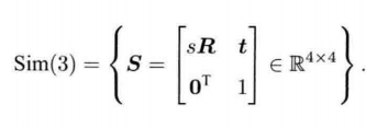
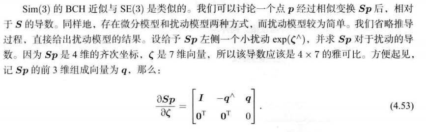
4.5 相似变换群 与 李代数
单目视觉 相似变换群Sim(3)
尺度不确定性 与 尺度漂移
对位于空间的点 p \bm{p} p ,在相机坐标系下要经过一个相似变换。
p ′ = [ s R t 0 T 1 ] p = s R p + t \bm{p}^{\prime}=\begin{bmatrix}s\bm{R} & \bm{t}\\ \bm{0}^T& 1 \end{bmatrix}\bm{p} = s\bm{Rp+t} p′=[sR0Tt1]p=sRp+t


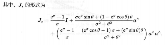

对于尺度因子,李群中的 s s s 即为李代数中 σ \sigma σ 的指数函数
4.6 小结
李群 SO(3) 和 SE(3) 以及对应的李代数 s o ( 3 ) \mathfrak{so}(3) so(3) 和 s e ( 3 ) \mathfrak{se}(3) se(3)
BCH 线性近似, 对位姿进行扰动并求导
习题


题1
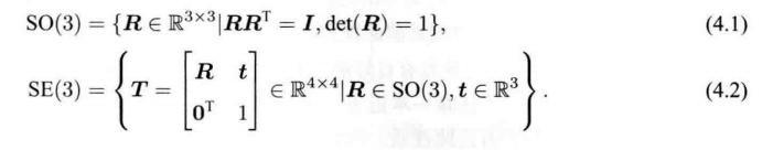
验证SO(3)、SE(3)、Sim(3)关于乘法成群
特殊正交群SO(n) 旋转矩阵群
特殊欧式群SE(n) n维欧式变换


题2

题4

√ 题5

证明:
原式等效于证明 R p ∧ R T R = ( R p ) ∧ R R p ∧ I = ( R p ) ∧ R R p ∧ = ( R p ) ∧ R 对于向量 v ∈ R 3 R p ∧ v = ( R p ) ∧ R v 上式等号左边 表示向量 p , v 叉乘后所得向量根据 R 旋转。 等号右边表示 向量 p , v 分别根据 R 旋转后叉乘,显然得到同一个向量。 证毕。 \begin{align*} 原式等效于证明\\ \bm{Rp^{\land}R^TR} & = \bm{(Rp)}^{\land}\bm{R} \\ \bm{Rp^{\land}\bm{I}} & = \bm{(Rp)}^{\land}\bm{R} \\ \bm{Rp^{\land}} & = \bm{(Rp)}^{\land}\bm{R} \\ 对于向量 \bm{v} \in \mathbb{R}^3\\ \bm{Rp^{\land}}\bm{v} & = \bm{(Rp)}^{\land}\bm{R}\bm{v} \\ 上式等号左边& 表示向量\bm{p,v}叉乘后所得向量根据 \bm{R}旋转。\\ 等号右边表示& 向量\bm{p,v}分别根据 \bm{R}旋转后叉乘,显然得到同一个向量。\\ 证毕。 \end{align*} 原式等效于证明Rp∧RTRRp∧IRp∧对于向量v∈R3Rp∧v上式等号左边等号右边表示证毕。=(Rp)∧R=(Rp)∧R=(Rp)∧R=(Rp)∧Rv表示向量p,v叉乘后所得向量根据R旋转。向量p,v分别根据R旋转后叉乘,显然得到同一个向量。
√ 题6
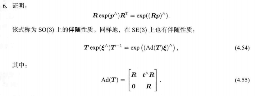
根据题 5 的结论 : ( R p ) ∧ = R p ∧ R T exp ( ( R p ) ∧ ) = exp ( R p ∧ R T ) 级数展开 = ∑ n = 0 ∞ ( R p ∧ R T ) n N ! = ∑ n = 0 ∞ R p ∧ R T ⋅ R p ∧ R T ⋅ , ⋅ ⋅ ⋅ , ⋅ R p ∧ R T ⋅ R p ∧ R T N ! 其中 R T R = I = ∑ n = 0 ∞ R ( p ∧ ) n R T N ! = R ∑ n = 0 ∞ ( p ∧ ) n N ! R T = R exp ( p ∧ ) R T \begin{align*}根据题5 的结论&:\bm{(Rp)}^{\land} = \bm{Rp^{\land}R^T} \\ \exp((\bm{Rp})^{\land})& = \exp(\bm{Rp^{\land}R^T}) \\ 级数展开\\ &= \sum\limits_{n=0}^{\infty}\frac{(\bm{Rp^{\land}R^T}) ^n}{N!} \\ &= \sum\limits_{n=0}^{\infty}\frac{\bm{Rp^{\land}R^T}·\bm{Rp^{\land}R^T}·,···,·\bm{Rp^{\land}R^T}·\bm{Rp^{\land}R^T}}{N!} \\ 其中 \bm{R^TR=I}\\ & = \sum\limits_{n=0}^{\infty}\frac{\bm{R(p^{\land})^nR^T}}{{N!} }\\ & = \bm{R} \sum\limits_{n=0}^{\infty}\frac{\bm{(p^{\land})^n}}{{N!} } \bm{R}^T \\ & = \bm{R}\exp(\bm{p}^{\land})\bm{R}^T \end{align*} 根据题5的结论exp((Rp)∧)级数展开其中RTR=I:(Rp)∧=Rp∧RT=exp(Rp∧RT)=n=0∑∞N!(Rp∧RT)n=n=0∑∞N!Rp∧RT⋅Rp∧RT⋅,⋅⋅⋅,⋅Rp∧RT⋅Rp∧RT=n=0∑∞N!R(p∧)nRT=Rn=0∑∞N!(p∧)nRT=Rexp(p∧)RT
证毕。
——————
6.2 SE(3)伴随性质
T exp ( ξ ∧ ) T − 1 = T ∑ n = 0 ∞ ( ξ ∧ ) n n ! T − 1 由于 T − 1 T = I = ∑ n = 0 ∞ T ξ ∧ T − 1 ⋅ T ξ ∧ T − 1 ⋅ T ξ ∧ T − 1 ⋅ T ξ ∧ T − 1 ⋅ , ⋅ ⋅ ⋅ , T ξ ∧ T − 1 ⋅ T ξ ∧ T − 1 n ! = ∑ n = 0 ∞ ( T ξ ∧ T − 1 ) n n ! = exp ( T ξ ∧ T − 1 ) \begin{align*} \bm{T}\exp(\bm{\xi}^{\land})\bm{T}^{-1} &= \bm{T}\sum\limits_{n=0}^{\infty}\frac{(\bm{\xi}^{\land})^n}{n!}\bm{T}^{-1} \\ 由于 \bm{T^{-1}T=I} \\ & = \sum\limits_{n=0}^{\infty}\frac{\bm{T}\bm{\xi}^{\land}\bm{T}^{-1}·\bm{T}\bm{\xi}^{\land}\bm{T}^{-1}·\bm{T}\bm{\xi}^{\land}\bm{T}^{-1}·\bm{T}\bm{\xi}^{\land}\bm{T}^{-1}·,···, \bm{T}\bm{\xi}^{\land}\bm{T}^{-1}·\bm{T}\bm{\xi}^{\land}\bm{T}^{-1}}{n!} \\ & = \sum\limits_{n=0}^{\infty}\frac{(\bm{T}\bm{\xi}^{\land}\bm{T}^{-1})^n}{n!} \\ &= \exp(\bm{T}\bm{\xi}^{\land}\bm{T}^{-1}) \\ \end{align*} Texp(ξ∧)T−1由于T−1T=I=Tn=0∑∞n!(ξ∧)nT−1=n=0∑∞n!Tξ∧T−1⋅Tξ∧T−1⋅Tξ∧T−1⋅Tξ∧T−1⋅,⋅⋅⋅,Tξ∧T−1⋅Tξ∧T−1=n=0∑∞n!(Tξ∧T−1)n=exp(Tξ∧T−1)
ξ = [ ρ ϕ ] , ξ ∧ = [ ϕ ∧ ρ 0 T 0 ] , T = [ R t 0 T 1 ] , T − 1 = [ R T − R T t 0 T 1 ] \bm{\xi=}\begin{bmatrix}\bm{\rho}\\ \bm{\phi} \end{bmatrix},\bm{\xi}^{\land}=\begin{bmatrix}\bm{\phi}^{\land} & \bm{\rho} \\ \bm{0}^T & 0 \end{bmatrix},\bm{T}=\begin{bmatrix}\bm{R} & \bm{t}\\ \bm{0}^T & 1 \end{bmatrix},\bm{T}^{-1}=\begin{bmatrix}\bm{R}^T & -\bm{R}^T\bm{t}\\ \bm{0}^T & 1 \end{bmatrix} ξ=[ρϕ],ξ∧=[ϕ∧0Tρ0],T=[R0Tt1],T−1=[RT0T−RTt1]

则:
T ξ ∧ T − 1 = [ R t 0 T 1 ] [ ϕ ∧ ρ 0 T 0 ] [ R T − R T t 0 T 1 ] = [ R ϕ ∧ R ρ 0 T 0 ] [ R T − R T t 0 T 1 ] = [ R ϕ ∧ R T − R ϕ ∧ R T t + R ρ 0 T 0 ] 由题 5 的结论 R p ∧ R T = ( R p ) ∧ = [ ( R ϕ ) ∧ − ( R ϕ ) ∧ t + R ρ 0 T 0 ] 对比 ξ , ξ ∧ 进行转换 = [ − ( R ϕ ) ∧ t + R ρ R ϕ ] ∧ 由叉乘性质, = [ t ∧ R ϕ + R ρ R ϕ ] ∧ = [ R t ∧ R 0 R ] [ ρ ϕ ] ) ∧ = ( A d ( T ) ξ ) ∧ \begin{align*}\bm{T}\bm{\xi}^{\land}\bm{T}^{-1}&= \begin{bmatrix}\bm{R} & \bm{t}\\ \bm{0}^T & 1 \end{bmatrix}\begin{bmatrix}\bm{\phi}^{\land} & \bm{\rho} \\ \bm{0}^T & 0 \end{bmatrix}\begin{bmatrix}\bm{R}^T & -\bm{R}^T\bm{t}\\ \bm{0}^T & 1 \end{bmatrix}\\ &= \begin{bmatrix}\bm{R}\bm{\phi}^{\land} & \bm{R\rho}\\ \bm{0}^T & 0 \end{bmatrix}\begin{bmatrix}\bm{R}^T & -\bm{R}^T\bm{t}\\ \bm{0}^T & 1 \end{bmatrix}\\ &= \begin{bmatrix}\bm{R}\bm{\phi}^{\land}\bm{R}^T & -\bm{R}\bm{\phi}^{\land}\bm{R}^T\bm{t + \bm{R\rho}}\\ \bm{0}^T & 0 \end{bmatrix} \\ 由题5的结论& \bm{Rp^{\land}R^T} = \bm{(Rp)}^{\land} \\ &= \begin{bmatrix}(\bm{R}\bm{\phi})^{\land} & -(\bm{R}\bm{\phi})^{\land}\bm{t + \bm{R\rho}}\\ \bm{0}^T &0 \end{bmatrix}\\ & 对比 \bm{\xi, {\xi}^{\land}}进行转换\\ &= \begin{bmatrix}-(\bm{R}\bm{\phi})^{\land}\bm{t + \bm{R\rho}}\\ \bm{R}\bm{\phi} \end{bmatrix}^{\land}\\ 由叉乘性质, \\ &= \begin{bmatrix}\bm{t}^{\land}\bm{R}\bm{\phi}+ \bm{R\rho}\\ \bm{R}\bm{\phi} \end{bmatrix}^{\land}\\ &= \begin{bmatrix}\bm{R}& \bm{t}^{\land}\bm{R} \\ \bm{0} & \bm{R} \end{bmatrix}\begin{bmatrix}\bm{\rho}\\ \bm{\phi} \end{bmatrix})^{\land}\\ & = (Ad(\bm{T})\bm{\xi})^{\land} \end{align*} Tξ∧T−1由题5的结论由叉乘性质,=[R0Tt1][ϕ∧0Tρ0][RT0T−RTt1]=[Rϕ∧0TRρ0][RT0T−RTt1]=[Rϕ∧RT0T−Rϕ∧RTt+Rρ0]Rp∧RT=(Rp)∧=[(Rϕ)∧0T−(Rϕ)∧t+Rρ0]对比ξ,ξ∧进行转换=[−(Rϕ)∧t+RρRϕ]∧=[t∧Rϕ+RρRϕ]∧=[R0t∧RR][ρϕ])∧=(Ad(T)ξ)∧
综上:
T exp ( ξ ∧ ) T − 1 = exp ( ( A d ( T ) ξ ) ∧ ) \bm{T}\exp(\bm{\xi}^{\land})\bm{T}^{-1}=\exp((Ad(\bm{T})\bm{\xi})^{\land}) Texp(ξ∧)T−1=exp((Ad(T)ξ)∧)
其中
A d ( T ) = [ R t ∧ R 0 R ] Ad(\bm{T})=\begin{bmatrix}\bm{R}& \bm{t}^{\land}\bm{R} \\ \bm{0} & \bm{R} \end{bmatrix} Ad(T)=[R0t∧RR]
证毕
————————————————
√ 题7


SO(3):
设右扰动 Δ R Δ\bm{R} ΔR 对应的李代数 为 φ \varphi φ
∂ ( R p ) ∂ φ = lim φ → 0 exp ( ϕ ∧ ) exp ( φ ∧ ) p − exp ( ϕ ∧ ) p φ = lim φ → 0 exp ( ϕ ∧ ) ( I + φ ∧ ) p − exp ( ϕ ∧ ) p φ = lim φ → 0 exp ( ϕ ∧ ) φ ∧ p φ = lim φ → 0 R φ ∧ p φ 由题 5 : R p ∧ = ( R p ) ∧ R = lim φ → 0 ( R φ ) ∧ R p φ 由叉乘性质 = lim φ → 0 − ( R p ) ∧ R φ φ = − ( R p ) ∧ R \begin{align*}\frac{\partial(\bm{Rp})}{\partial\varphi} &= \lim\limits_{\varphi\to0}\frac{\exp(\phi^{\land})\exp(\varphi^{\land})\bm{p}-\exp(\phi^{\land})\bm{p}}{\varphi}\\ &= \lim\limits_{\varphi\to0}\frac{\exp(\phi^{\land})(\bm{I} + \varphi^{\land})\bm{p}-\exp(\phi^{\land})\bm{p}}{\varphi}\\ &= \lim\limits_{\varphi\to0}\frac{\exp(\phi^{\land})\varphi^{\land}\bm{p}}{\varphi}\\ &= \lim\limits_{\varphi\to0}\frac{\bm{R}\varphi^{\land}\bm{p}}{\varphi}\\ 由题5 : \bm{Rp^{\land}} & = \bm{(Rp)}^{\land}\bm{R} \\ &= \lim\limits_{\varphi\to0}\frac{(\bm{R}\varphi)^{\land}\bm{Rp}}{\varphi}\\ 由叉乘性质\\ &= \lim\limits_{\varphi\to0}\frac{-(\bm{Rp})^{\land}\bm{R}\varphi}{\varphi}\\ & = -(\bm{Rp})^{\land}\bm{R} \end{align*} ∂φ∂(Rp)由题5:Rp∧由叉乘性质=φ→0limφexp(ϕ∧)exp(φ∧)p−exp(ϕ∧)p=φ→0limφexp(ϕ∧)(I+φ∧)p−exp(ϕ∧)p=φ→0limφexp(ϕ∧)φ∧p=φ→0limφRφ∧p=(Rp)∧R=φ→0limφ(Rφ)∧Rp=φ→0limφ−(Rp)∧Rφ=−(Rp)∧R
SE(3):
假设某空间点 p \bm{p} p 经过一次变换 T \bm{T} T (对应李代数为 ξ \bm{\xi} ξ), 得到 T p \bm{Tp} Tp
现在给 T \bm{T} T 右乘一个扰动 Δ T = exp ( Δ ξ ∧ ) Δ\bm{T} = \exp(Δ\bm{\xi}^{\land}) ΔT=exp(Δξ∧)
设扰动项的李代数为 Δ ξ = [ Δ ρ , Δ ϕ ] T Δ\bm{\xi}=[Δ\bm{\rho},Δ\bm{\phi}]^T Δξ=[Δρ,Δϕ]T,则
∂ ( T p ) ∂ Δ ξ = lim Δ ξ → 0 exp ( ξ ∧ ) exp ( Δ ξ ∧ ) p − exp ( ξ ∧ ) p Δ ξ = lim Δ ξ → 0 exp ( ξ ∧ ) ( I + Δ ξ ∧ ) p − exp ( ξ ∧ ) p Δ ξ = lim Δ ξ → 0 exp ( ξ ∧ ) Δ ξ ∧ p Δ ξ = lim Δ ξ → 0 [ R t 0 1 ] [ Δ ϕ ∧ Δ ρ 0 T 0 ] p Δ ξ 把 p 前的 矩阵当做旋转矩阵,结合向量旋转的性质, = lim Δ ξ → 0 [ R t 0 1 ] [ Δ ϕ ∧ p + Δ ρ 0 ] Δ ξ = lim Δ ξ → 0 [ R Δ ϕ ∧ p + R Δ ρ 0 T ] [ Δ ρ , Δ ϕ ] T 将 Δ ρ , Δ ϕ 提出来,方便求导 根据 R p ∧ = ( R p ) ∧ R = lim Δ ξ → 0 [ ( R Δ ϕ ) ∧ R p + R Δ ρ 0 T ] [ Δ ρ , Δ ϕ ] T = lim Δ ξ → 0 [ − ( R p ) ∧ R Δ ϕ + R Δ ρ 0 T ] [ Δ ρ , Δ ϕ ] T = [ R − ( R p ) ∧ R 0 T 0 T ] \begin{align*}\frac{\partial(\bm{Tp})}{\partial{Δ\bm{\xi}}} &= \lim\limits_{Δ\bm{\xi}\to0}\frac{\exp(\bm{\xi}^{\land})\exp(Δ\bm{\xi}^{\land})\bm{p}-\exp(\bm{\xi}^{\land})\bm{p}}{Δ\bm{\xi}} \\ &= \lim\limits_{Δ\bm{\xi}\to0}\frac{\exp(\bm{\xi}^{\land})(\bm{I} +Δ\bm{\xi}^{\land})\bm{p}-\exp(\bm{\xi}^{\land})\bm{p}}{Δ\bm{\xi}} \\ &= \lim\limits_{Δ\bm{\xi}\to0}\frac{\exp(\bm{\xi}^{\land})Δ\bm{\xi}^{\land}\bm{p}}{Δ\bm{\xi}} \\ &=\lim\limits_{Δ\bm{\xi}\to0} \frac{\begin{bmatrix} \bm{R} & \bm{t}\\ 0 & 1 \end{bmatrix}\begin{bmatrix} Δ\bm{\phi}^{\land} & \Delta\bm{\rho}\\ \bm{0}^T & 0 \end{bmatrix}\bm{p}}{Δ\bm{\xi}}\\ 把\bm{p}前的&矩阵当做旋转矩阵,结合向量旋转的性质,\\ &=\lim\limits_{Δ\bm{\xi}\to0} \frac{\begin{bmatrix} \bm{R} & \bm{t}\\ 0 & 1 \end{bmatrix}\begin{bmatrix} Δ\bm{\phi}^{\land}\bm{p} + \Delta\bm{\rho}\\ 0 \end{bmatrix}}{Δ\bm{\xi}}\\ &=\lim\limits_{Δ\bm{\xi}\to0} \frac{\begin{bmatrix} \bm{R}\Delta\bm{\phi}^{\land}\bm{p}+ \bm{R}\Delta\bm{\rho}\\ \bm{0}^T \end{bmatrix}}{[Δ\bm{\rho},Δ\bm{\phi}]^T} \\ 将&Δ\bm{\rho},Δ\bm{\phi} 提出来,方便求导\\ & 根据 \bm{Rp^{\land}} = \bm{(Rp)}^{\land}\bm{R} \\ &=\lim\limits_{Δ\bm{\xi}\to0} \frac{\begin{bmatrix} (\bm{R}\Delta\bm{\phi})^{\land}\bm{R}\bm{p}+\bm{R}\Delta\bm{\rho}\\ \bm{0}^T \end{bmatrix}}{[Δ\bm{\rho},Δ\bm{\phi}]^T} \\ &=\lim\limits_{Δ\bm{\xi}\to0} \frac{\begin{bmatrix} -(\bm{R}\bm{p})^{\land}\bm{R}\Delta\bm{\phi}+ \bm{R}\Delta\bm{\rho}\\ \bm{0}^T \end{bmatrix}}{[Δ\bm{\rho},Δ\bm{\phi}]^T} \\ & = \begin{bmatrix} \bm{R} & -(\bm{R}\bm{p})^{\land}\bm{R} \\ \bm{0}^T & \bm{0}^T \end{bmatrix} \\ \end{align*} ∂Δξ∂(Tp)把p前的将=Δξ→0limΔξexp(ξ∧)exp(Δξ∧)p−exp(ξ∧)p=Δξ→0limΔξexp(ξ∧)(I+Δξ∧)p−exp(ξ∧)p=Δξ→0limΔξexp(ξ∧)Δξ∧p=Δξ→0limΔξ[R0t1][Δϕ∧0TΔρ0]p矩阵当做旋转矩阵,结合向量旋转的性质,=Δξ→0limΔξ[R0t1][Δϕ∧p+Δρ0]=Δξ→0lim[Δρ,Δϕ]T[RΔϕ∧p+RΔρ0T]Δρ,Δϕ提出来,方便求导根据Rp∧=(Rp)∧R=Δξ→0lim[Δρ,Δϕ]T[(RΔϕ)∧Rp+RΔρ0T]=Δξ→0lim[Δρ,Δϕ]T[−(Rp)∧RΔϕ+RΔρ0T]=[R0T−(Rp)∧R0T]
——————————————
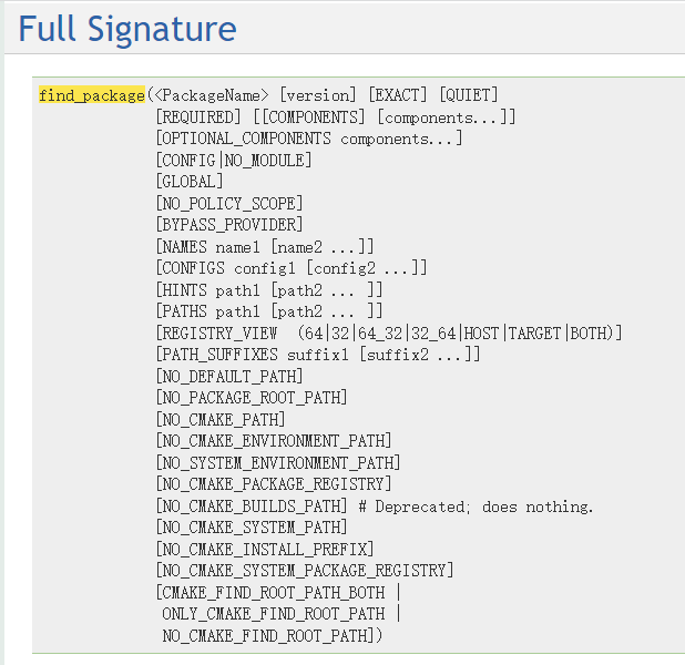
√ 题8
cmake的 find_package指令:
官方文档
find_package(包名 版本 REQUIRED)
一些包需要 sudo make install后才能被找到

LaTex
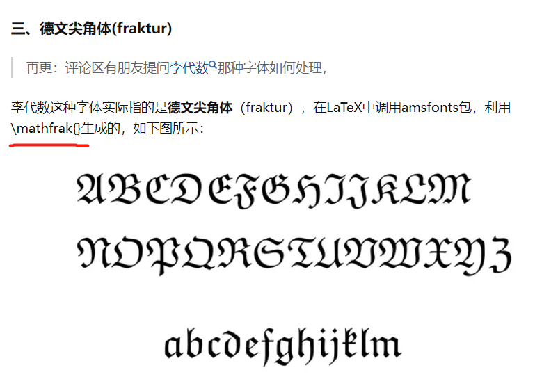
$\mathfrak{g}$
g \mathfrak{g} g
$\mathbb{R}$
R \mathbb{R} R
$\times$
× \times ×
$\varphi$
φ \varphi φ
$\Phi$
Φ \Phi Φ
$\overset{\mathrm{def}}{=}$
$\xlongequal{def}$
= d e f \overset{\mathrm{def}}{=} =def
= d e f \xlongequal{def} def
相关文章:
《视觉 SLAM 十四讲》V2 第 4 讲 李群与李代数 【什么样的相机位姿 最符合 当前观测数据】
P71 文章目录 4.1 李群与李代数基础4.1.3 李代数的定义4.1.4 李代数 so(3)4.1.5 李代数 se(3) 4.2 指数与对数映射4.2.1 SO(3)上的指数映射罗德里格斯公式推导 4.2.2 SE(3) 上的指数映射SO(3),SE(3),so(3),se(3)的对应关系 4.3 李代数求导与扰动模型4.3.2 SO(3)上的李代数求导…...
【深蓝学院】手写VIO第4章--基于滑动窗口算法的 VIO 系统:可观性和 一致性--笔记
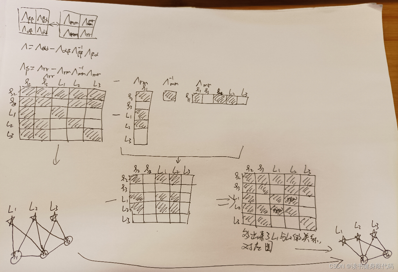
0. 内容 T1. 参考SLAM14讲P247直接可写,注意 ξ 1 , ξ 2 \xi_1,\xi_2 ξ1,ξ2之间有约束(关系)。 套用舒尔补公式: marg掉 ξ 1 \xi_1 ξ1之后,信息被传递到 L 1 和 L 2 L_1和L_2 L1和L2之间了。 T2....

mfc 动态加载dll库,Mat转CImage,读ini配置文件,鼠标操作,在edit控件上画框,调试信息打印
动态加载dll库 h文件中添加 #include "mydll.h" #ifdef UNICODE //区分字符集 #define LoadLibrary LoadLibraryW #else #define LoadLibrary LoadLibraryA #endif // !UNICODEtypedef double(*mydllPtr)(int, int);类内添加: mydllPtr m_mydll; cpp…...
索尼 toio™应用创意开发征文|检测工业平台震动
虽然索尼toio Q宝机器人主要是为儿童教育娱乐开发的,但我认为它在工业等领域也有一定应用潜力。例如,工业领域经常会有某些平面在实际作业中持续震动,导致零件过疲劳、平台失去稳定等问题。而这样的平台往往位于机器内部,从外部很…...
【已解决】 Expected linebreaks to be ‘LF‘ but found ‘CRLF‘.
问题描述 团队都是用mac,只有我自己是windows,启动项目一直报错 Expected linebreaks to be ‘LF‘ but found ‘CRLF‘. 但我不能因为自己的问题去改团队配置,也尝试过该vscode配置默认是LF还是报错 思路 看文章vscode如何替换所有文件的…...

Java8 Lambda.stream.sorted() 方法使用浅析分享
文章目录 Java8 Lambda.stream.sorted() 方法使用浅析分享sorted() 重载方法一升序降序 sorted() 重载方法二升序降序多字段排序 mock代码 Java8 Lambda.stream.sorted() 方法使用浅析分享 本文主要分享运用 Java8 中的 Lambda.stream.sorted方法排序的使用! sorted…...
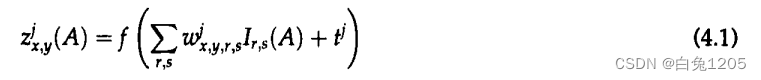
Neural Networks for Fingerprint Recognition
Neural Computation ( IF 3.278 ) 摘要: 在采集指纹图像数据库后,设计了一种用于指纹识别的神经网络算法。当给出一对指纹图像时,算法输出两个图像来自同一手指的概率估计值。在一个实验中,神经网络使用几百对图像进行训练&…...

ChatGPT推出全新功能,引发人工智能合成声音担忧|百能云芯
人工智能AI科技企业OpenAI公司25日宣布,其聊天应用程序ChatGPT如今具备「看、听、说」能力,至少能够理解口语、用合成语音回应并且处理图像;但专家忧心,以假乱真与深度伪造的乱象可能变本加厉。 国家广播公司新闻网(NBC News)报导…...
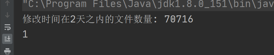
Java 实现遍历一个文件夹,文件夹有100万数据,获取到修改时间在2天之内的数据
目录 1 需求2 实现1(第一种方法)2 实现2 (推荐使用这个,快)3 实现3(推荐) 1 需求 现在有一个文件夹,里面会一直存数据,动态的存数据,之后可能会达到100万&am…...

持续集成部署-k8s-命令行工具:基础命令的使用
持续集成部署-k8s-命令行工具:基础命令的使用 1. 资源类型与别名2. 资源操作2.1 创建对象2.2 显示和查找资源2.3 更新资源2.4 修补资源2.5 编辑资源2.6 scale 资源2.7 删除资源3. 格式化输出1. 资源类型与别名 资源类型缩写别名clusterscomponentstatusescsconfigmapscmdaemon…...
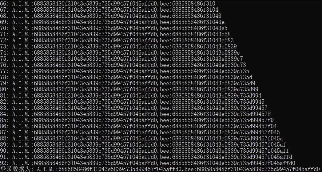
使用python脚本的时间盲注完整步骤
文章目录 一、获取数据库名称长度二、获取数据库名称三、获取表名总长度四、获取表名五、获取指定表列名总长度六、获取指定表列名七、获取指定表指定列的表内数据总长度八、获取指定表指定列的表内数据 一、获取数据库名称长度 测试环境是bwapp靶场 SQL Injection - Blind - …...
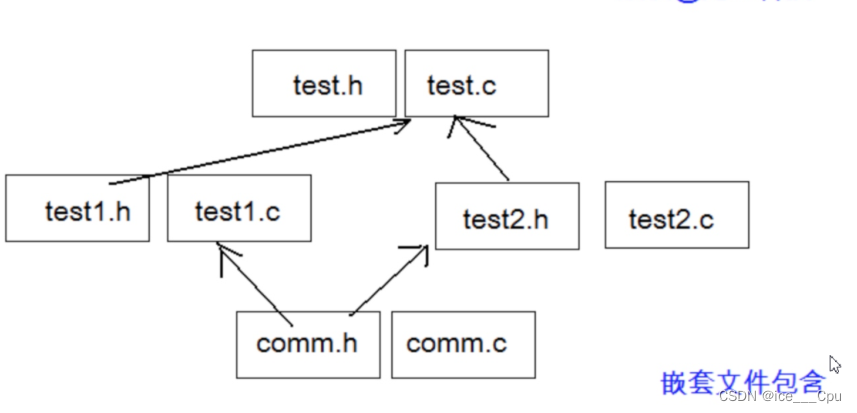
C++项目:仿mudou库one thread one loop式并发服务器实现
目录 1.实现目标 2.HTTP服务器 3.Reactor模型 3.1分类 4.功能模块划分: 4.1SERVER模块: 4.2HTTP协议模块: 5.简单的秒级定时任务实现 5.1Linux提供给我们的定时器 5.2时间轮思想: 6.正则库的简单使用 7.通用类型any类型的实现 8.日志宏的实现 9.缓冲区…...
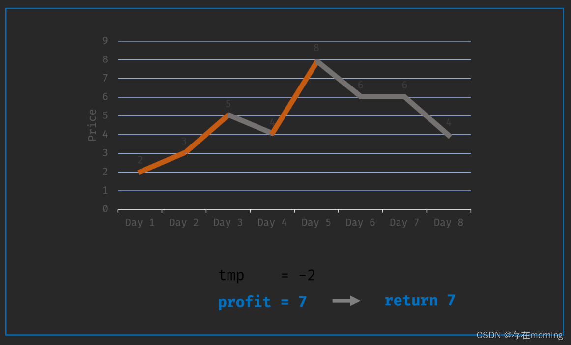
【算法训练-贪心算法 一】买卖股票的最佳时机II
废话不多说,喊一句号子鼓励自己:程序员永不失业,程序员走向架构!本篇Blog的主题是【贪心算法】,使用【数组】这个基本的数据结构来实现,这个高频题的站点是:CodeTop,筛选条件为&…...

单阶段目标检测与双阶段目标检测的联系与区别
🚀 作者 :“码上有钱” 🚀 文章简介 :AI-目标检测算法 🚀 欢迎小伙伴们 点赞👍、收藏⭐、留言💬简介 双阶段目标检测算法与单阶段目标检测算法在工作原理和性能方面存在一些相似与差异之处。下…...

Mysql技术文档--设计表规范式-一次性扫盲
阿丹: 在设计表的时候经常出现一些问题,其实自己很清楚就是因为在设计表的时候没有规范。导致后期加表的时候出现了问题。所以趁着这个假期卷一卷。同时只有在开始的时候 几大范式 在关系型数据库中,数据表设计的基本原则、规则就称为范式。…...

python socket 传输opencv读取的图像
python socket网络编程 将ros机器人摄像头捕捉的画面在上位机实时显示,需要用到socket网络编程,提供了TCP和UDP两种方式 TCP服务器端代码: 创建TCP套接字: s socket(AF_INET, SOCK_STREAM) 创建了一个TCP套接字。SOCK_STREAM 表示这是一个TCP套接字&…...

APACHE NIFI学习之—UpdateAttribute
UpdateAttribute 描述: 通过设置属性表达式来更新属性,也可以基于属性正则匹配来删除属性 标签: attributes, modification, update, delete, Attribute Expression Language, state, 属性, 修改, 更新, 删除, 表达式 参数: 如下列表中,必填参数则…...
BIT-7文件操作和程序环境(16000字详解)
一:文件 1.1 文件指针 每个被使用的文件都在内存中开辟了一个相应的文件信息区,用来存放文件的相关信息(如文件的名字,文件状态及文件当前的位置等)。这些信息是保存在一个结构体变量中的。该结构体类型是有系统声明…...

冥想第九百二十八天
1.今天周三,今天晚上日语课上了好久,天气也不好, 2.项目上全力以赴的一天。 3.感谢父母,感谢朋友感谢家人,感谢不断进步的自己。...
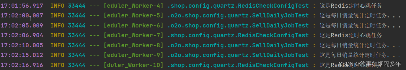
深入浅出,SpringBoot整合Quartz实现定时任务与Redis健康检测(一)
目录 前言 环境配置 Quartz 什么是Quartz? 应用场景 核心组件 Job JobDetail Trigger CronTrigger SimpleTrigger Scheduler 任务存储 RAM JDBC 导入依赖 定时任务 销量统计 Redis检测 使用 编辑 注意事项 前言 在悦享校园1.0中引入了Quart…...

基于agent-foundry框架构建智能体:从核心原理到天气助手实战
1. 项目概述:从零构建你的智能体开发框架最近在GitHub上看到一个挺有意思的项目,叫hebertzhu/agent-foundry。乍一看名字,你可能会觉得这又是一个跟风大语言模型热潮的“又一个Agent框架”。但当我真正深入去研究它的代码结构、设计理念和实际…...

ImageGlass:Windows平台最强图像浏览器,90+格式全支持
ImageGlass:Windows平台最强图像浏览器,90格式全支持 【免费下载链接】ImageGlass 🏞 A lightweight, versatile image viewer 项目地址: https://gitcode.com/gh_mirrors/im/ImageGlass 你是否曾因Windows自带照片应用无法打开专业RA…...

Helm模板智能助手:提升Kubernetes应用部署效率的VSCode插件
1. 为什么你需要一个Helm模板智能助手如果你和我一样,每天都在和Kubernetes的Helm Charts打交道,那你一定对编写templates/目录下那些.yaml文件又爱又恨。爱的是Helm的模板引擎确实强大,能把一堆重复的YAML配置抽象成可复用的模板;…...

EmbedClaw:RAG应用中文本智能分块与向量化检索的工程实践
1. 项目概述:一个面向嵌入向量检索的“机械爪”最近在折腾RAG(检索增强生成)应用,发现向量数据库的检索效果,很大程度上取决于你“喂”进去的文本是怎么被切成一块一块的(也就是分块,Chunking&a…...

松下绿色科技战略:技术复用与协同效应如何驱动企业转型
1. 松下困局:消费电子巨头的十字路口2013年初的拉斯维加斯,消费电子展(CES)的喧嚣与霓虹之下,松下的时任社长津贺一宏站在聚光灯前,面对的却是一个冰冷而残酷的现实:公司预计将连续第二年录得高…...

VSCode写Verilog效率翻倍:除了语法检查,再教你用Python插件自动生成模块例化
VSCode写Verilog效率翻倍:Python插件自动化实战指南 在FPGA开发中,Verilog代码的重复性劳动往往消耗工程师大量时间。我曾在一个图像处理项目中被模块例化折磨得焦头烂额——手动编写30多个相同结构的FIFO例化代码,不仅容易出错,后…...

MCP协议实战:构建AI智能体任务管理服务器与二次开发指南
1. 项目概述:一个为AI智能体“开眼”的MCP服务器最近在折腾AI智能体(Agent)开发的朋友,估计都绕不开一个词:MCP。全称是Model Context Protocol,你可以把它理解为给大模型(比如Claude、GPT-4&am…...

AI赋能二进制安全:BinAIVulHunter项目实战与逆向工程集成
1. 项目概述与核心价值最近在安全圈里,一个名为BinAIVulHunter的开源项目引起了我的注意。这个项目名直译过来就是“二进制AI漏洞猎人”,光看名字就能猜到它的核心玩法:利用人工智能技术,来自动化分析二进制文件,挖掘其…...
)
【仅开放72小时】:Gemini Workspace与Microsoft Entra ID双向同步的密钥轮换脚本(含自动审计日志生成器)
更多请点击: https://intelliparadigm.com 第一章:Gemini Workspace整合方案概述 Gemini Workspace 是 Google 推出的面向企业级 AI 协作的统一平台,其核心价值在于将 Gemini 模型能力深度嵌入办公套件(如 Gmail、Drive、Docs、M…...

AI信息摘要工具:从数据采集到智能推送的完整实践指南
1. 项目概述:一个AI驱动的每日信息摘要工具最近在GitHub上看到一个挺有意思的项目,叫“ai-daily-digest”。光看名字,你大概能猜到它的核心功能:利用人工智能技术,自动为你生成每日的信息摘要。作为一个经常被信息洪流…...