[Machine learning][Part4] 多维矩阵下的梯度下降线性预测模型的实现
目录
模型初始化信息:
模型实现:
多变量损失函数:
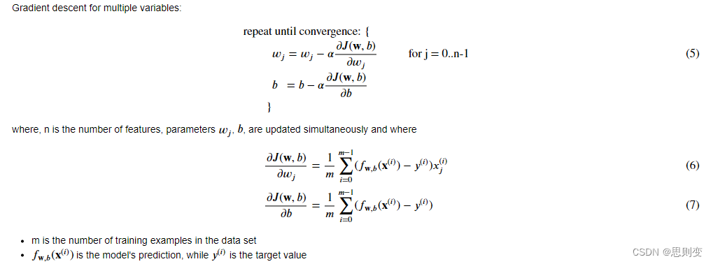
多变量梯度下降实现:
多变量梯度实现:
多变量梯度下降实现:
之前部分实现的梯度下降线性预测模型中的training example只有一个特征属性:房屋面积,这显然是不符合实际情况的,这里增加特征属性的数量再实现一次梯度下降线性预测模型。
这里回顾一下梯度下降线性模型的实现方法:
- 实现线性模型:f = w*x + b,模型参数w,b待定
- 寻找最优的w,b组合:
(1)引入衡量模型优劣的cost function:J(w,b) ——损失函数或者代价函数
(2)损失函数值最小的时候,模型最接近实际情况:通过梯度下降法来寻找最优w,b组合
模型初始化信息:
- 新的房子的特征有:房子面积、卧室数、楼层数、房龄共4个特征属性。
| Size (sqft) | Number of Bedrooms | Number of floors | Age of Home | Price (1000s dollars) |
|---|---|---|---|---|
| 2104 | 5 | 1 | 45 | 460 |
| 1416 | 3 | 2 | 40 | 232 |
| 852 | 2 | 1 | 35 | 17 |
上面表中的训练样本有3个,输入特征矩阵模型为:
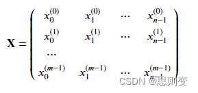
具体代码实现为,X_train是输入矩阵,y_train是输出矩阵
X_train = np.array([[2104, 5, 1, 45], [1416, 3, 2, 40],[852, 2, 1, 35]])
y_train = np.array([460, 232, 178])
模型参数w,b矩阵:
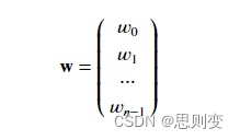
代码实现:w中的每一个元素对应房屋的一个特征属性
b_init = 785.1811367994083
w_init = np.array([ 0.39133535, 18.75376741, -53.36032453, -26.42131618])
模型实现:
def predict(x, w, b): """single predict using linear regressionArgs:x (ndarray): Shape (n,) example with multiple featuresw (ndarray): Shape (n,) model parameters b (scalar): model parameter Returns:p (scalar): prediction"""p = np.dot(x, w) + b return p 多变量损失函数:
J(w,b)为:
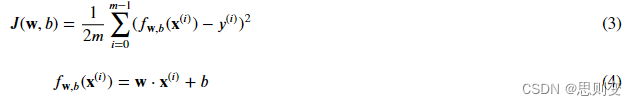
代码实现为:
def compute_cost(X, y, w, b): """compute costArgs:X (ndarray (m,n)): Data, m examples with n featuresy (ndarray (m,)) : target valuesw (ndarray (n,)) : model parameters b (scalar) : model parameterReturns:cost (scalar): cost"""m = X.shape[0]cost = 0.0for i in range(m): f_wb_i = np.dot(X[i], w) + b #(n,)(n,) = scalar (see np.dot)cost = cost + (f_wb_i - y[i])**2 #scalarcost = cost / (2 * m) #scalar return cost多变量梯度下降实现:
多变量梯度实现:
def compute_gradient(X, y, w, b): """Computes the gradient for linear regression Args:X (ndarray (m,n)): Data, m examples with n featuresy (ndarray (m,)) : target valuesw (ndarray (n,)) : model parameters b (scalar) : model parameterReturns:dj_dw (ndarray (n,)): The gradient of the cost w.r.t. the parameters w. dj_db (scalar): The gradient of the cost w.r.t. the parameter b. """m,n = X.shape #(number of examples, number of features)dj_dw = np.zeros((n,))dj_db = 0.for i in range(m): err = (np.dot(X[i], w) + b) - y[i] for j in range(n): dj_dw[j] = dj_dw[j] + err * X[i, j] dj_db = dj_db + err dj_dw = dj_dw / m dj_db = dj_db / m return dj_db, dj_dw多变量梯度下降实现:
def gradient_descent(X, y, w_in, b_in, cost_function, gradient_function, alpha, num_iters): """Performs batch gradient descent to learn theta. Updates theta by taking num_iters gradient steps with learning rate alphaArgs:X (ndarray (m,n)) : Data, m examples with n featuresy (ndarray (m,)) : target valuesw_in (ndarray (n,)) : initial model parameters b_in (scalar) : initial model parametercost_function : function to compute costgradient_function : function to compute the gradientalpha (float) : Learning ratenum_iters (int) : number of iterations to run gradient descentReturns:w (ndarray (n,)) : Updated values of parameters b (scalar) : Updated value of parameter """# An array to store cost J and w's at each iteration primarily for graphing laterJ_history = []w = copy.deepcopy(w_in) #avoid modifying global w within functionb = b_infor i in range(num_iters):# Calculate the gradient and update the parametersdj_db,dj_dw = gradient_function(X, y, w, b) ##None# Update Parameters using w, b, alpha and gradientw = w - alpha * dj_dw ##Noneb = b - alpha * dj_db ##None# Save cost J at each iterationif i<100000: # prevent resource exhaustion J_history.append( cost_function(X, y, w, b))# Print cost every at intervals 10 times or as many iterations if < 10if i% math.ceil(num_iters / 10) == 0:print(f"Iteration {i:4d}: Cost {J_history[-1]:8.2f} ")return w, b, J_history #return final w,b and J history for graphing梯度下降算法测试:
# initialize parameters
initial_w = np.zeros_like(w_init)
initial_b = 0.
# some gradient descent settings
iterations = 1000
alpha = 5.0e-7
# run gradient descent
w_final, b_final, J_hist = gradient_descent(X_train, y_train, initial_w, initial_b,compute_cost, compute_gradient, alpha, iterations)
print(f"b,w found by gradient descent: {b_final:0.2f},{w_final} ")
m,_ = X_train.shape
for i in range(m):print(f"prediction: {np.dot(X_train[i], w_final) + b_final:0.2f}, target value: {y_train[i]}")# plot cost versus iteration
fig, (ax1, ax2) = plt.subplots(1, 2, constrained_layout=True, figsize=(12, 4))
ax1.plot(J_hist)
ax2.plot(100 + np.arange(len(J_hist[100:])), J_hist[100:])
ax1.set_title("Cost vs. iteration");  ax2.set_title("Cost vs. iteration (tail)")
ax1.set_ylabel('Cost')             ;  ax2.set_ylabel('Cost')
ax1.set_xlabel('iteration step')   ;  ax2.set_xlabel('iteration step')
plt.show()
结果为:
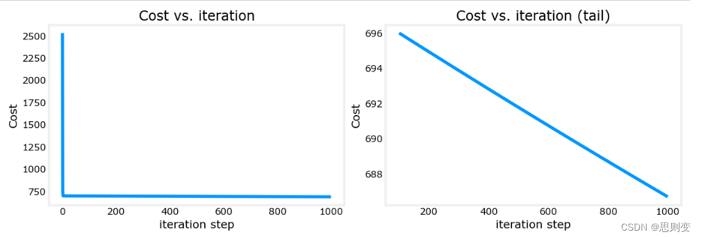
可以看到,右图中损失函数在traning次数结束之后还一直在下降,没有找到最佳的w,b组合。具体解决方法,后面会有更新。
完整的代码为:
import copy, math
import numpy as np
import matplotlib.pyplot as pltnp.set_printoptions(precision=2)  # reduced display precision on numpy arraysX_train = np.array([[2104, 5, 1, 45], [1416, 3, 2, 40], [852, 2, 1, 35]])
y_train = np.array([460, 232, 178])b_init = 785.1811367994083
w_init = np.array([ 0.39133535, 18.75376741, -53.36032453, -26.42131618])def predict(x, w, b):"""single predict using linear regressionArgs:x (ndarray): Shape (n,) example with multiple featuresw (ndarray): Shape (n,) model parametersb (scalar):             model parameterReturns:p (scalar):  prediction"""p = np.dot(x, w) + breturn pdef compute_cost(X, y, w, b):"""compute costArgs:X (ndarray (m,n)): Data, m examples with n featuresy (ndarray (m,)) : target valuesw (ndarray (n,)) : model parametersb (scalar)       : model parameterReturns:cost (scalar): cost"""m = X.shape[0]cost = 0.0for i in range(m):f_wb_i = np.dot(X[i], w) + b  # (n,)(n,) = scalar (see np.dot)cost = cost + (f_wb_i - y[i]) ** 2  # scalarcost = cost / (2 * m)  # scalarreturn costdef compute_gradient(X, y, w, b):"""Computes the gradient for linear regressionArgs:X (ndarray (m,n)): Data, m examples with n featuresy (ndarray (m,)) : target valuesw (ndarray (n,)) : model parametersb (scalar)       : model parameterReturns:dj_dw (ndarray (n,)): The gradient of the cost w.r.t. the parameters w.dj_db (scalar):       The gradient of the cost w.r.t. the parameter b."""m, n = X.shape  # (number of examples, number of features)dj_dw = np.zeros((n,))dj_db = 0.for i in range(m):err = (np.dot(X[i], w) + b) - y[i]for j in range(n):dj_dw[j] = dj_dw[j] + err * X[i, j]dj_db = dj_db + errdj_dw = dj_dw / mdj_db = dj_db / mreturn dj_db, dj_dwdef gradient_descent(X, y, w_in, b_in, cost_function, gradient_function, alpha, num_iters):"""Performs batch gradient descent to learn theta. Updates theta by takingnum_iters gradient steps with learning rate alphaArgs:X (ndarray (m,n))   : Data, m examples with n featuresy (ndarray (m,))    : target valuesw_in (ndarray (n,)) : initial model parametersb_in (scalar)       : initial model parametercost_function       : function to compute costgradient_function   : function to compute the gradientalpha (float)       : Learning ratenum_iters (int)     : number of iterations to run gradient descentReturns:w (ndarray (n,)) : Updated values of parametersb (scalar)       : Updated value of parameter"""# An array to store cost J and w's at each iteration primarily for graphing laterJ_history = []w = copy.deepcopy(w_in)  # avoid modifying global w within functionb = b_infor i in range(num_iters):# Calculate the gradient and update the parametersdj_db, dj_dw = gradient_function(X, y, w, b)  ##None# Update Parameters using w, b, alpha and gradientw = w - alpha * dj_dw  ##Noneb = b - alpha * dj_db  ##None# Save cost J at each iterationif i < 100000:  # prevent resource exhaustionJ_history.append(cost_function(X, y, w, b))# Print cost every at intervals 10 times or as many iterations if < 10if i % math.ceil(num_iters / 10) == 0:print(f"Iteration {i:4d}: Cost {J_history[-1]:8.2f}   ")return w, b, J_history  # return final w,b and J history for graphing# initialize parameters
initial_w = np.zeros_like(w_init)
initial_b = 0.
# some gradient descent settings
iterations = 1000
alpha = 5.0e-7
# run gradient descent
w_final, b_final, J_hist = gradient_descent(X_train, y_train, initial_w, initial_b,compute_cost, compute_gradient,alpha, iterations)
print(f"b,w found by gradient descent: {b_final:0.2f},{w_final} ")
m,_ = X_train.shape
for i in range(m):print(f"prediction: {np.dot(X_train[i], w_final) + b_final:0.2f}, target value: {y_train[i]}")# plot cost versus iteration
fig, (ax1, ax2) = plt.subplots(1, 2, constrained_layout=True, figsize=(12, 4))
ax1.plot(J_hist)
ax2.plot(100 + np.arange(len(J_hist[100:])), J_hist[100:])
ax1.set_title("Cost vs. iteration");  ax2.set_title("Cost vs. iteration (tail)")
ax1.set_ylabel('Cost')             ;  ax2.set_ylabel('Cost')
ax1.set_xlabel('iteration step')   ;  ax2.set_xlabel('iteration step')
plt.show()
相关文章:
[Machine learning][Part4] 多维矩阵下的梯度下降线性预测模型的实现
目录 模型初始化信息: 模型实现: 多变量损失函数: 多变量梯度下降实现: 多变量梯度实现: 多变量梯度下降实现: 之前部分实现的梯度下降线性预测模型中的training example只有一个特征属性:…...

LCR 078. 合并 K 个升序链表
LCR 078. 合并 K 个升序链表 题目链接:LCR 078. 合并 K 个升序链表 代码如下: class Solution { public:ListNode* mergeKLists(vector<ListNode*>& lists) {ListNode *lsnullptr;for(int i0;i<lists.size();i){lsmergeList(ls,lists[i])…...
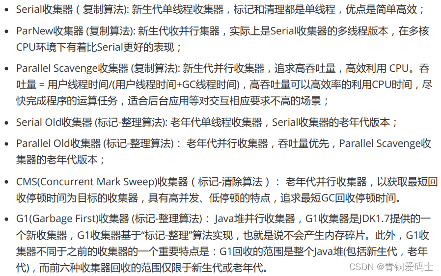
JVM面试题:(三)GC和垃圾回收算法
GC: 垃圾回收算法: GC最基础的算法有三种: 标记 -清除算法、复制算法、标记-压缩算法,我们常用的垃圾回收器一般 都采用分代收集算法。 标记 -清除算法,“标记-清除”(Mark-Sweep)算法,如它的…...
)
hive建表指定列分隔符为多字符分隔符实战(默认只支持单字符)
1、背景: 后端日志采集完成,清洗入hive表的过程中,发现字段之间的单一字符的分割符号已经不能满足列分割需求,因为字段值本身可能包含分隔符。所以列分隔符使用多个字符列分隔符迫在眉睫。 hive在建表时,通常使用ROW …...

android.app.RemoteServiceException: can‘t deliver broadcast
日常报错记录 android.app.RemoteServiceException: cant deliver broadcast W BroadcastQueue: Cant deliver broadcast to com.broadcast.test(pid 1769). Crashing it.E AndroidRuntime: FATAL EXCEPTION: main E AndroidRuntime: Process: com.broadcast.test, PID: 1769…...
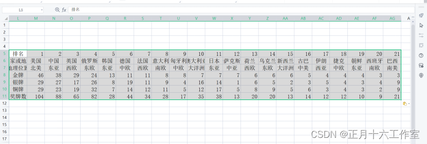
信创办公–基于WPS的EXCEL最佳实践系列 (单元格与行列)
信创办公–基于WPS的EXCEL最佳实践系列 (单元格与行列) 目录 应用背景操作步骤1、插入和删除行和列2、合并单元格3、调整行高与列宽4、隐藏行与列5、修改单元格对齐和缩进6、更改字体7、使用格式刷8、设置单元格内的文本自动换行9、应用单元格样式10、插…...
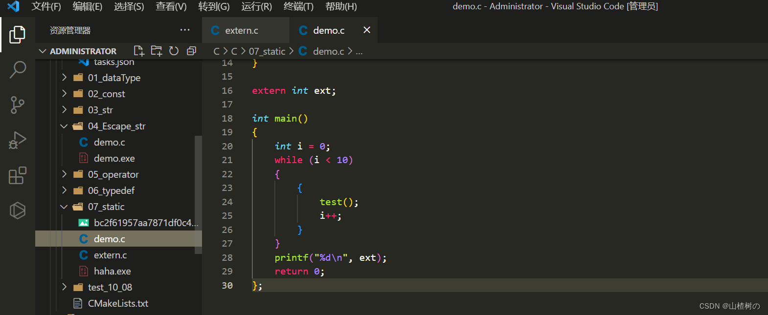
VsCode同时编译多个C文件
VsCode默认只能编译单个C文件,想要编译多个文件,需要额外进行配置 第一种方法 ——> 通过手动指定要编译的文件 g -g .\C文件1 .\C文件2 -o 编译后exe名称 例如我将demo.c和extern.c同时编译得到haha.exe g -g .\demo.c .\extern.c -o haha 第二种…...

Android绑定式服务
Github:https://github.com/MADMAX110/Odometer 启动式服务对于后台操作很合适,不过需要一个更有交互性的服务。 接下来构建这样一个应用: 1、创建一个绑定式服务的基本版本,名为OdometerService 我们要为它增加一个方法getDistance()&#x…...

系统韧性研究(1)| 何谓「系统韧性」?
过去十年,系统韧性作为一个关键问题被广泛讨论,在数据中心和云计算方面尤甚,同时它对赛博物理系统也至关重要,尽管该术语在该领域不太常用。大伙都希望自己的系统具有韧性,但这到底意味着什么?韧性与其他质…...

使用Perl脚本编写爬虫程序的一些技术问题解答
网络爬虫是一种强大的工具,用于从互联网上收集和提取数据。Perl 作为一种功能强大的脚本语言,提供了丰富的工具和库,使得编写的爬虫程序变得简单而灵活。在使用的过程中大家会遇到一些问题,本文将通过问答方式,解答一些…...
SAP内部转移价格(利润中心转移价格)的条件
SAP内部转移价格(利润中心转移价格) SAP内部转移价格(利润中心转移价格) SAP内部转移价格(利润中心转移价格)这个听了很多人说过,但是利润中心转移定价需要具备什么条件。没有找到具体的文档。…...

WRF如何批量输出文件添加或删除文件名后缀
1. 批量添加文件名后缀 #1----批量添加文件名后缀(.nc)。#指定wrfout文件所在的文件夹 path "/mnt/wtest1/"#列出路径path下所有的文件 file_names os.listdir(path) #遍历在path路径下所有以wrfout_d01开头的文件,在os.path…...
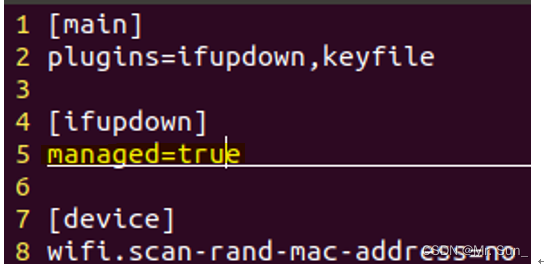
Ubuntu右上角不显示网络的图标解决办法
一.line5改为true sudo vim /etc/NetworkManager/NetworkManager.conf 二.重启网卡 sudo service network-manager stop sudo mv /var/lib/NetworkManager/NetworkManager.state /tmp sudo service network-manager start...

AM@数列极限
文章目录 abstract极限👺极限的主要问题 数列极限数列极限的定义 ( ϵ − N ) (\epsilon-N) (ϵ−N)语言描述极限表达式成立的证明极限发散证明常用数列极限数列极限的几何意义例 函数的极限 abstract 数列极限 极限👺 极限分为数列的极限和函数的极限…...
Vue-2.3v-model原理
原理:v-model本质上是一个语法糖,例如应用在输入框上,就是value属性和input事件的合写。 作用:提供数据的双向绑定 1)数据变,视图跟着变:value 2)视图变,数据跟着变input 注意&a…...

左手 Serverless,右手 AI,7 年躬身的古籍修复之路
作者:宋杰 “AI 可以把我们思维体系当中,过度专业化、过度细分的这些所谓的知识都替代掉,让我们集中精力去体验自己的生命。我挺幸运的,代码能够有 AI 辅助,也能够有 Serverless 解决我的运营成本问题。Serverless 它…...

计算mask的体素数量
import numpy as np import nibabel as nib # 用于处理神经影像数据的库 # 从文件中加载mask图像 mask_image nib.load(rE:\mask.nii.gz) # 获取图像数据 mask_data mask_image.get_fdata() # 计算非零像素的数量,即白质骨架的体素总数 voxel_count np.count_no…...

VR全景营销颠覆传统营销,让消费者身临其境
随着VR的普及,各种VR产品、功能开始层出不穷,并且在多个领域都有落地应用,例如文旅、景区、酒店、餐饮、工厂、地产、汽车等,在这个“内容为王”的时代,VR全景展示也是一种新的内容表达方式。 VR全景营销让消费者沉浸式…...
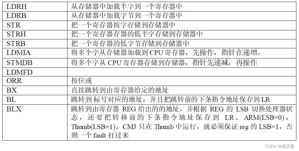
FreeRTOS学习笔记——四、任务的定义与任务切换的实现
FreeRTOS学习笔记——四、任务的定义与任务切换的实现 0 前言1 什么是任务2 创建任务2.1 定义任务栈2.2 定义任务函数2.3 定义任务控制块2.4 实现任务创建函数2.4.1 任务创建函数 —— xTaskCreateStatic()函数2.4.2 创建新任务——prvInitialiseNewTask()函数2.4.3 初始化任务…...
js 之让人迷惑的闭包 03
文章目录 一、闭包是什么? 🤦♂️二、闭包 😎三、使用场景 😁四、使用场景(2) 😁五、闭包的原理六、思考总结一、 更深层次了解闭包,分析以下代码执行过程二、闭包三、闭包定义四、…...

AMLP:基于大语言模型的自动化机器学习势函数构建平台
1. 项目概述:当AI遇见原子模拟,AMLP如何重塑机器学习势函数构建在计算材料科学和化学物理领域,分子动力学模拟是我们窥探微观世界动态行为的“显微镜”。无论是研究新材料的相变过程,还是探索生物大分子的折叠机制,其核…...

Godot中型项目工程化实践:目录规范、资源引用与状态管理
1. 这不是续集,而是项目落地的分水岭“Godot 游戏引擎项目(二)”——看到这个标题,很多人第一反应是:“哦,上一篇讲了环境搭建和Hello World,这篇该讲节点树和信号了?”但我在带三个…...

Python PIL 画矩形框
基础代码 from PIL import Image, ImageDraw# 打开图片 img Image.open(your_image.jpg)# 创建绘图对象 draw ImageDraw.Draw(img)# 矩形坐标 (x1, y1, x2, y2) coords (23, 21, 69, 76)# 画矩形框(红色,线宽2) draw.rectangle(coords, ou…...

rk35xx 通过recovery升级问题
Firefly 的 recovery 库是一个核心组件,它构建了一个独立的微型 Linux 系统,专门用于在设备主系统之外执行高可靠性的固件升级。简单来说,它的工作流程是:主系统通过命令触发,将升级指令写入特定分区并重启;…...
)
保姆级教程:Windows系统下Arcgis 10.2从下载、安装到汉化一次搞定(附常见License启动失败解决方案)
Windows系统下Arcgis 10.2完整安装与汉化实战指南第一次接触Arcgis的新手往往会被复杂的安装流程和神秘的License Manager搞得晕头转向。作为一款功能强大的地理信息系统软件,Arcgis在科研、城市规划、环境监测等领域有着广泛应用,但它的安装过程确实会让…...

XML 服务器
XML 服务器 引言 XML(可扩展标记语言)服务器在现代互联网技术中扮演着至关重要的角色。它为数据的传输和处理提供了灵活且高效的方式。本文将深入探讨XML服务器的概念、工作原理、应用场景及其在软件开发中的重要性。 什么是XML服务器? XML服务器是一种用于存储、处理和…...

网络配置工具类详解
CNet 网络配置工具类详解平台:仅支持 Linux,大量使用 ioctl 系统调用一、概述 CNet 是一个 纯静态方法的网络配置工具类,封装了 Linux 下常用的网络操作:功能类别涵盖内容IP 地址读取/设置本机 IP、子网掩码网关读取/添加/删除/设…...

第三卷第4章:原型模式设计思想
第三卷第4章:原型模式设计思想 目录介绍 01.案例引入与思考 1.1 痛点场景 1.2 它哪里不舒服 1.3 引出本篇主角 02.原型模式介绍 2.1 原型模式由来 2.2 原型模式定义...

完整指南:如何在5分钟内快速上手BioAge生物年龄计算工具包
完整指南:如何在5分钟内快速上手BioAge生物年龄计算工具包 【免费下载链接】BioAge Biological Age Calculations Using Several Biomarker Algorithms 项目地址: https://gitcode.com/gh_mirrors/bi/BioAge BioAge生物年龄计算工具包是一款基于R语言开发的强…...

独立开发者利用taotoken模型广场为不同任务选择性价比最优模型
🚀 告别海外账号与网络限制!稳定直连全球优质大模型,限时半价接入中。 👉 点击领取海量免费额度 独立开发者利用taotoken模型广场为不同任务选择性价比最优模型 对于独立开发者而言,在有限的预算内高效完成多样化的开…...