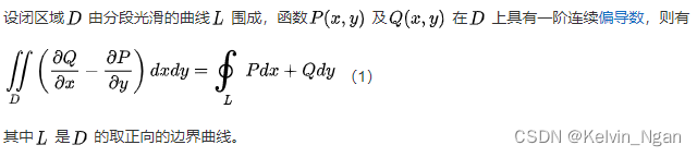
关于opencv的contourArea计算方法
cv::contourArea计算的轮廓面积并不等于轮廓点计数,原因是cv::contourArea是基于Green公式计算
老外的讨论 github
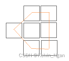
举一个直观的例子,图中有7个像素,橙色为轮廓点连线,按照contourArea的定义,轮廓的面积为橙色所包围的区域=3
以下代码基于opencv4.8.0
cv::contourArea源码位于.\sources\modules\imgproc\src\shapedescr.cpp
// area of a whole sequence
double cv::contourArea( InputArray _contour, bool oriented )
{CV_INSTRUMENT_REGION();Mat contour = _contour.getMat();int npoints = contour.checkVector(2);int depth = contour.depth();CV_Assert(npoints >= 0 && (depth == CV_32F || depth == CV_32S));if( npoints == 0 )return 0.;double a00 = 0;bool is_float = depth == CV_32F;const Point* ptsi = contour.ptr<Point>();const Point2f* ptsf = contour.ptr<Point2f>();Point2f prev = is_float ? ptsf[npoints-1] : Point2f((float)ptsi[npoints-1].x, (float)ptsi[npoints-1].y);for( int i = 0; i < npoints; i++ ){Point2f p = is_float ? ptsf[i] : Point2f((float)ptsi[i].x, (float)ptsi[i].y);a00 += (double)prev.x * p.y - (double)prev.y * p.x;prev = p;}a00 *= 0.5;if( !oriented )a00 = fabs(a00);return a00;
}
如果计算面积需要考虑轮廓点本身,可以通过cv::drawContoursI填充轮廓获得mask图像后统计非零点个数
cv::drawContours源码位于.\sources\modules\imgproc\src\drawing.cpp,主要包括两步:收集边缘cv::CollectPolyEdges和填充边缘cv::FillEdgeCollection,How does the drawContours function work in OpenCV when a contour is filled?
struct PolyEdge
{PolyEdge() : y0(0), y1(0), x(0), dx(0), next(0) {}//PolyEdge(int _y0, int _y1, int _x, int _dx) : y0(_y0), y1(_y1), x(_x), dx(_dx) {}int y0, y1;int64 x, dx;PolyEdge *next;
};static void
CollectPolyEdges( Mat& img, const Point2l* v, int count, std::vector<PolyEdge>& edges,const void* color, int line_type, int shift, Point offset )
{int i, delta = offset.y + ((1 << shift) >> 1);Point2l pt0 = v[count-1], pt1;pt0.x = (pt0.x + offset.x) << (XY_SHIFT - shift);pt0.y = (pt0.y + delta) >> shift;edges.reserve( edges.size() + count );for( i = 0; i < count; i++, pt0 = pt1 ){Point2l t0, t1;PolyEdge edge;pt1 = v[i];pt1.x = (pt1.x + offset.x) << (XY_SHIFT - shift);pt1.y = (pt1.y + delta) >> shift;Point2l pt0c(pt0), pt1c(pt1);if (line_type < cv::LINE_AA){t0.y = pt0.y; t1.y = pt1.y;t0.x = (pt0.x + (XY_ONE >> 1)) >> XY_SHIFT;t1.x = (pt1.x + (XY_ONE >> 1)) >> XY_SHIFT;Line(img, t0, t1, color, line_type);// use clipped endpoints to create a more accurate PolyEdgeif ((unsigned)t0.x >= (unsigned)(img.cols) ||(unsigned)t1.x >= (unsigned)(img.cols) ||(unsigned)t0.y >= (unsigned)(img.rows) ||(unsigned)t1.y >= (unsigned)(img.rows)){clipLine(img.size(), t0, t1);if (t0.y != t1.y){pt0c.y = t0.y; pt1c.y = t1.y;pt0c.x = (int64)(t0.x) << XY_SHIFT;pt1c.x = (int64)(t1.x) << XY_SHIFT;}}else{pt0c.x += XY_ONE >> 1;pt1c.x += XY_ONE >> 1;}}else{t0.x = pt0.x; t1.x = pt1.x;t0.y = pt0.y << XY_SHIFT;t1.y = pt1.y << XY_SHIFT;LineAA(img, t0, t1, color);}if (pt0.y == pt1.y)continue;edge.dx = (pt1c.x - pt0c.x) / (pt1c.y - pt0c.y);if (pt0.y < pt1.y){edge.y0 = (int)(pt0.y);edge.y1 = (int)(pt1.y);edge.x = pt0c.x + (pt0.y - pt0c.y) * edge.dx; // correct starting point for clipped lines}else{edge.y0 = (int)(pt1.y);edge.y1 = (int)(pt0.y);edge.x = pt1c.x + (pt1.y - pt1c.y) * edge.dx; // correct starting point for clipped lines}edges.push_back(edge);}
}struct CmpEdges
{bool operator ()(const PolyEdge& e1, const PolyEdge& e2){return e1.y0 - e2.y0 ? e1.y0 < e2.y0 :e1.x - e2.x ? e1.x < e2.x : e1.dx < e2.dx;}
};static void
FillEdgeCollection( Mat& img, std::vector<PolyEdge>& edges, const void* color, int line_type)
{PolyEdge tmp;int i, y, total = (int)edges.size();Size size = img.size();PolyEdge* e;int y_max = INT_MIN, y_min = INT_MAX;int64 x_max = 0xFFFFFFFFFFFFFFFF, x_min = 0x7FFFFFFFFFFFFFFF;int pix_size = (int)img.elemSize();int delta;if (line_type < CV_AA)delta = 0;elsedelta = XY_ONE - 1;if( total < 2 )return;for( i = 0; i < total; i++ ){PolyEdge& e1 = edges[i];CV_Assert( e1.y0 < e1.y1 );// Determine x-coordinate of the end of the edge.// (This is not necessary x-coordinate of any vertex in the array.)int64 x1 = e1.x + (e1.y1 - e1.y0) * e1.dx;y_min = std::min( y_min, e1.y0 );y_max = std::max( y_max, e1.y1 );x_min = std::min( x_min, e1.x );x_max = std::max( x_max, e1.x );x_min = std::min( x_min, x1 );x_max = std::max( x_max, x1 );}if( y_max < 0 || y_min >= size.height || x_max < 0 || x_min >= ((int64)size.width<<XY_SHIFT) )return;std::sort( edges.begin(), edges.end(), CmpEdges() );// start drawingtmp.y0 = INT_MAX;edges.push_back(tmp); // after this point we do not add// any elements to edges, thus we can use pointersi = 0;tmp.next = 0;e = &edges[i];y_max = MIN( y_max, size.height );for( y = e->y0; y < y_max; y++ ){PolyEdge *last, *prelast, *keep_prelast;int draw = 0;int clipline = y < 0;prelast = &tmp;last = tmp.next;while( last || e->y0 == y ){if( last && last->y1 == y ){// exclude edge if y reaches its lower pointprelast->next = last->next;last = last->next;continue;}keep_prelast = prelast;if( last && (e->y0 > y || last->x < e->x) ){// go to the next edge in active listprelast = last;last = last->next;}else if( i < total ){// insert new edge into active list if y reaches its upper pointprelast->next = e;e->next = last;prelast = e;e = &edges[++i];}elsebreak;if( draw ){if( !clipline ){// convert x's from fixed-point to image coordinatesuchar *timg = img.ptr(y);int x1, x2;if (keep_prelast->x > prelast->x){x1 = (int)((prelast->x + delta) >> XY_SHIFT);x2 = (int)(keep_prelast->x >> XY_SHIFT);}else{x1 = (int)((keep_prelast->x + delta) >> XY_SHIFT);x2 = (int)(prelast->x >> XY_SHIFT);}// clip and draw the lineif( x1 < size.width && x2 >= 0 ){if( x1 < 0 )x1 = 0;if( x2 >= size.width )x2 = size.width - 1;ICV_HLINE( timg, x1, x2, color, pix_size );}}keep_prelast->x += keep_prelast->dx;prelast->x += prelast->dx;}draw ^= 1;}// sort edges (using bubble sort)keep_prelast = 0;do{prelast = &tmp;last = tmp.next;PolyEdge *last_exchange = 0;while( last != keep_prelast && last->next != 0 ){PolyEdge *te = last->next;// swap edgesif( last->x > te->x ){prelast->next = te;last->next = te->next;te->next = last;prelast = te;last_exchange = prelast;}else{prelast = last;last = te;}}if (last_exchange == NULL)break;keep_prelast = last_exchange;} while( keep_prelast != tmp.next && keep_prelast != &tmp );}
}
其中填充算法为scan-line polygon filling algorithm,下面转载该文
Polygon Filling? How do you do that?
In order to fill a polygon, we do not want to have to determine the type of polygon that we are filling. The easiest way to avoid this situation is to use an algorithm that works for all three types of polygons. Since both convex and concave polygons are subsets of the complex type, using an algorithm that will work for complex polygon filling should be sufficient for all three types. The scan-line polygon fill algorithm, which employs the odd/even parity concept previously discussed, works for complex polygon filling.
Reminder: The basic concept of the scan-line algorithm is to draw points from edges of odd parity to even parity on each scan-line.
What is a scan-line? A scan-line is a line of constant y value, i.e., y=c, where c lies within our drawing region, e.g., the window on our computer screen.
The scan-line algorithm is outlined next.
When filling a polygon, you will most likely just have a set of vertices, indicating the x and y Cartesian coordinates of each vertex of the polygon. The following steps should be taken to turn your set of vertices into a filled polygon.
1.Initializing All of the Edges:
The first thing that needs to be done is determine how the polygon’s vertices are related. The all_edges table will hold this information.
Each adjacent set of vertices (the first and second, second and third, …, last and first) defines an edge. For each edge, the following information needs to be kept in a table:
缩进 1.The minimum y value of the two vertices.
缩进 2.The maximum y value of the two vertices.
缩进 3.The x value associated with the minimum y value.
缩进 4.The slope of the edge.
The slope of the edge can be calculated from the formula for a line:
y = mx + b;
where m = slope, b = y-intercept,
y0 = maximum y value,
y1 = minimum y value,
x0 = maximum x value,
x1 = minimum x value
The formula for the slope is as follows:
m = (y0 - y1) / (x0 - x1).
For example, the edge values may be kept as follows, where N is equal to the total number of edges - 1 and each index into the all_edges array contains a pointer to the array of edge values.
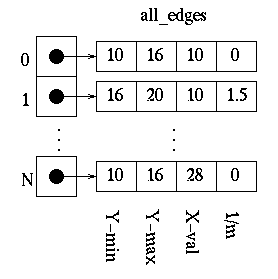
2.Initializing the Global Edge Table:
The global edge table will be used to keep track of the edges that are still needed to complete the polygon. Since we will fill the edges from bottom to top and left to right. To do this, the global edge table table should be inserted with edges grouped by increasing minimum y values. Edges with the same minimum y values are sorted on minimum x values as follows:
缩进 1.Place the first edge with a slope that is not equal to zero in the global edge table.
缩进 2.If the slope of the edge is zero, do not add that edge to the global edge table.
缩进 3.For every other edge, start at index 0 and increase the index to the global edge table once each time the current edge’s y value is greater than that of the edge at the current index in the global edge table.
Next, Increase the index to the global edge table once each time the current edge’s x value is greater than and the y value is less than or equal to that of the edge at the current index in the global edge table.
If the index, at any time, is equal to the number of edges currently in the global edge table, do not increase the index.
Place the edge information for minimum y value, maximum y value, x value, and 1/m in the global edge table at the index.
The global edge table should now contain all of the edge information necessary to fill the polygon in order of increasing minimum y and x values.
3.Initializing Parity
The initial parity is even since no edges have been crossed yet.
4.Initializing the Scan-Line
The initial scan-line is equal to the lowest y value for all of the global edges. Since the global edge table is sorted, the scan-line is the minimum y value of the first entry in this table.
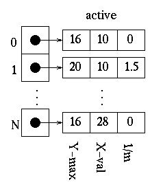
5.Initializing the Active Edge Table
The active edge table will be used to keep track of the edges that are intersected by the current scan-line. This should also contain ordered edges. This is initially set up as follows:
Since the global edge table is ordered on minimum y and x values, search, in order, through the global edge table and, for each edge found having a minimum y value equal to the current scan-line, append the edge information for the maximum y value, x value, and 1/m to the active edge table. Do this until an edge is found with a minimum y value greater than the scan line value. The active edge table will now contain ordered edges of those edges that are being filled as such:
6.Filling the Polygon
Filling the polygon involves deciding whether or not to draw pixels, adding to and removing edges from the active edge table, and updating x values for the next scan-line.
Starting with the initial scan-line, until the active edge table is empty, do the following:
缩进 1.Draw all pixels from the x value of odd to the x value of even parity edge pairs.
缩进 2.Increase the scan-line by 1.
缩进 3.Remove any edges from the active edge table for which the maximum y value is equal to the scan_line.
缩进 4.Update the x value for for each edge in the active edge table using the formula x1 = x0 + 1/m. (This is based on the line formula and the fact that the next scan-line equals the old scan-line plus one.)
缩进 5.Remove any edges from the global edge table for which the minimum y value is equal to the scan-line and place them in the active edge table.
缩进 6.Reorder the edges in the active edge table according to increasing x value. This is done in case edges have crossed.
相关文章:
关于opencv的contourArea计算方法
cv::contourArea计算的轮廓面积并不等于轮廓点计数,原因是cv::contourArea是基于Green公式计算 老外的讨论 github 举一个直观的例子,图中有7个像素,橙色为轮廓点连线,按照contourArea的定义,轮廓的面积为橙色所包围…...
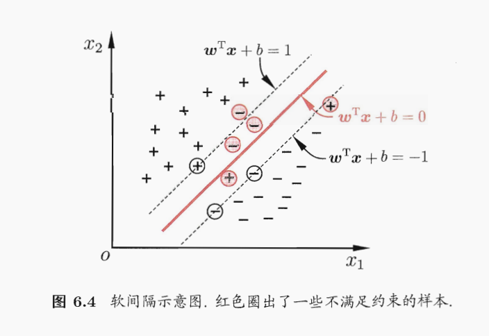
《机器学习》第6章 支持向量机
文章目录 6.1 间隔与支持向量6.2 对偶问题6.3 核函数支持向量展式核函数 6.4 软间隔与正则化6.5 支持向量回归6.6 核方法6.7 阅读材料 6.1 间隔与支持向量 分类学习最基本的想法就是基于训练集D在样本空间中找到一个划分超平面,将不同类别的样本分开.但能将训练样本分开的划分…...
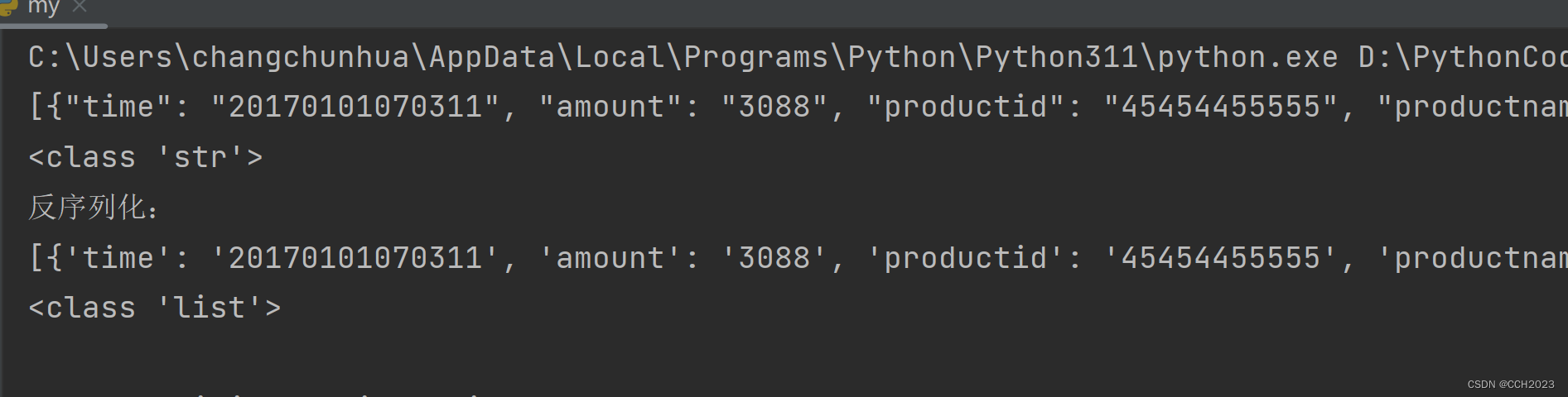
Python学习基础笔记七十七——json序列化
客户端和服务端之间需要交换数据才能完成各种功能。 假设 服务端程序都是用Python语言开发的话,那么 服务端从数据库中获取的最近的交易列表,可能就是像下面这样的一个Python列表对象: historyTransactions [{time : 20170101070311, #…...

【C++】C++11新特性
文章目录 一、C发展简介二、C11简介三、列表初始化1.统一使用{}初始化2.initializer_list类 四、变量的类型推导1.auto2.decltype3.nullptr 五、范围for循环六、STL中一些变化七、final与override八、新的类功能1.新增默认成员函数2.成员变量的缺省值3.default 和 delete4.fina…...
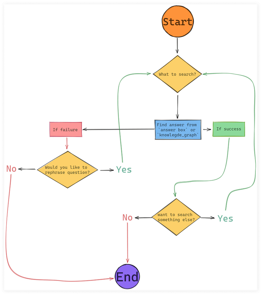
使用 PyAudio、语音识别、pyttsx3 和 SerpApi 构建简单的基于 CLI 的语音助手
德米特里祖布☀️ 一、介绍 正如您从标题中看到的,这是一个演示项目,显示了一个非常基本的语音助手脚本,可以根据 Google 搜索结果在终端中回答您的问题。 您可以在 GitHub 存储库中找到完整代码:dimitryzub/serpapi-demo-project…...
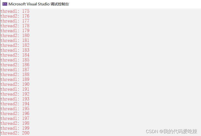
C++11——多线程
目录 一.thread类的简单介绍 二.线程函数参数 三.原子性操作库(atomic) 四.lock_guard与unique_lock 1.lock_guard 2.unique_lock 五.条件变量 一.thread类的简单介绍 在C11之前,涉及到多线程问题,都是和平台相关的,比如windows和linu…...
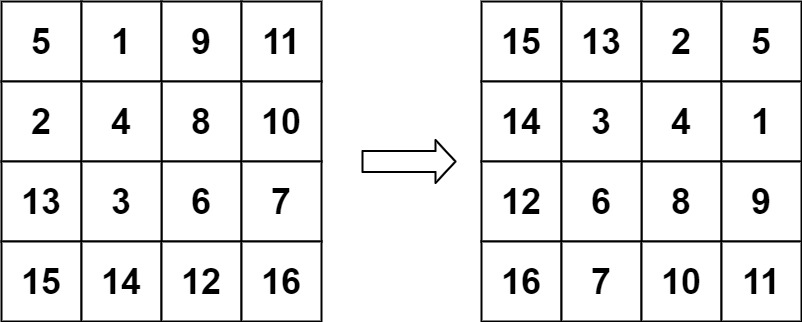
力扣每日一题48:旋转图像
题目描述: 给定一个 n n 的二维矩阵 matrix 表示一个图像。请你将图像顺时针旋转 90 度。 你必须在 原地 旋转图像,这意味着你需要直接修改输入的二维矩阵。请不要 使用另一个矩阵来旋转图像。 示例 1: 输入:matrix [[1,2,3],…...
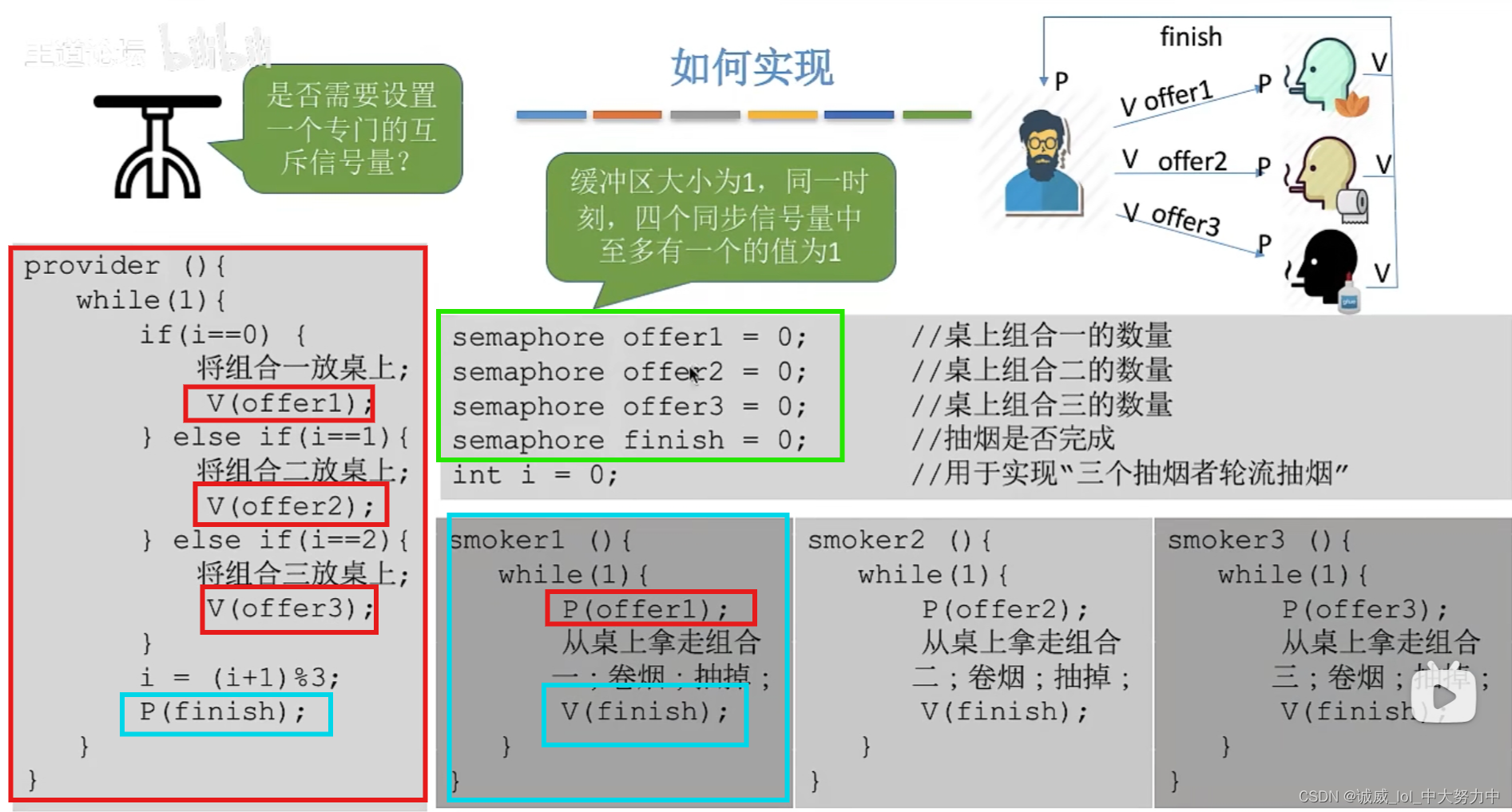
操作系统——吸烟者问题(王道视频p34、课本ch6)
1.问题分析:这个问题可以看作是 可以生产多种产品的 单生产者-多消费者问题 2.代码——这里就是由于同步信号量的初值都是1,所以没有使用mutex互斥信号, 总共4个同步信号量,其中一个是 finish信号量...
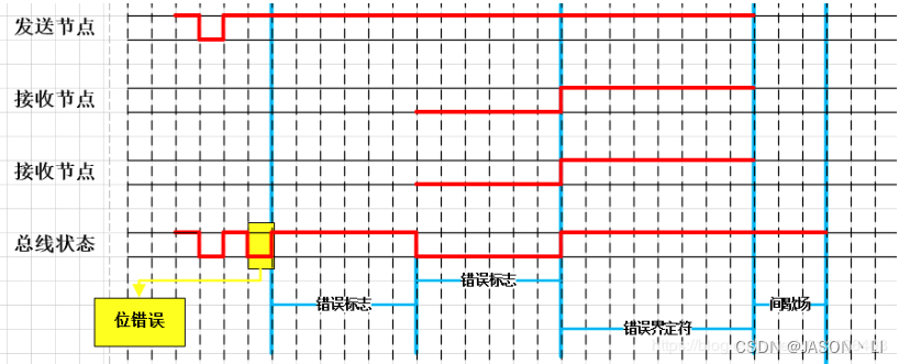
通讯协议学习之路:CAN协议理论
通讯协议之路主要分为两部分,第一部分从理论上面讲解各类协议的通讯原理以及通讯格式,第二部分从具体运用上讲解各类通讯协议的具体应用方法。 后续文章会同时发表在个人博客(jason1016.club)、CSDN;视频会发布在bilibili(UID:399951374) 序、…...
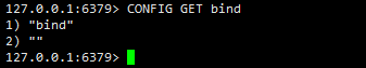
Redis常用配置详解
目录 一、Redis查看当前配置命令二、Redis基本配置三、RDB全量持久化配置(默认开启)四、AOF增量持久化配置五、Redis key过期监听配置六、Redis内存淘汰策略七、总结 一、Redis查看当前配置命令 # Redis查看当前全部配置信息 127.0.0.1:6379> CONFIG…...
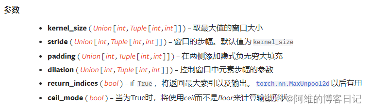
卷积神经网络CNN学习笔记-MaxPool2D函数解析
目录 1.函数签名:2.学习中的疑问3.代码 1.函数签名: torch.nn.MaxPool2d(kernel_size, strideNone, padding0, dilation1, return_indicesFalse, ceil_modeFalse) 2.学习中的疑问 Q:使用MaxPool2D池化时,当卷积核移动到某位置,该卷积核覆盖区域超过了输入尺寸时,MaxPool2D会…...

基于图像字典学习的去噪技术研究与实践
图像去噪是计算机视觉领域的一个重要研究方向,其目标是从受到噪声干扰的图像中恢复出干净的原始图像。字典学习是一种常用的图像去噪方法,它通过学习图像的稀疏表示字典,从而实现对图像的去噪处理。本文将详细介绍基于字典学习的图像去噪技术…...
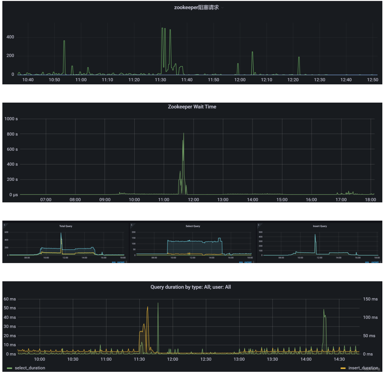
记一次Clickhouse 复制表同步延迟排查
现象 数据从集群中一个节点写入之后,其他两个节点无法及时查询到数据,等了几分钟。因为我们ck集群是读写分离架构,也就是一个节点写数据,其他节点供读取。 排查思路 从业务得知,数据更新时间点为:11:30。…...

Maven的详细安装步骤说明
Step 1: 下载Maven 首先,您需要从Maven官方网站(https://maven.apache.org/)下载Maven的最新版本。在下载页面上,找到与您操作系统对应的二进制文件(通常是.zip或.tar.gz格式),下载到本地。 St…...
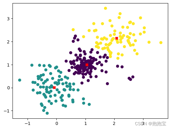
金融机器学习方法:K-均值算法
目录 1.算法介绍 2.算法原理 3.python实现示例 1.算法介绍 K均值聚类算法是机器学习和数据分析中常用的无监督学习方法之一,主要用于数据的分类。它的目标是将数据划分为几个独特的、互不重叠的子集或“集群”,以使得同一集群内的数据点彼此相似&…...
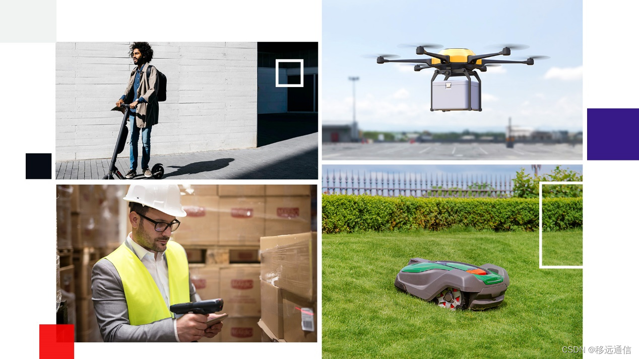
移远通信携手MIKROE推出搭载LC29H系列模组的Click boards开发板,为物联网应用带来高精定位服务
近日,移远通信与MikroElektronika(以下简称“MIKROE”)展开合作,基于移远LC29H系列模组推出了多款支持实时动态载波相位差分技术(RTK)和惯性导航(DR)技术的Click Boards™ 开发板&am…...
Spring Cloud 之 Sentinel简介与GATEWAY整合实现
简介 随着微服务的流行,服务和服务之间的稳定性变得越来越重要。Sentinel 是面向分布式服务架构的流量控制组件,主要以流量为切入点,从限流、流量整形、熔断降级、系统负载保护、热点防护等多个维度来帮助开发者保障微服务的稳定性。 熔断 …...
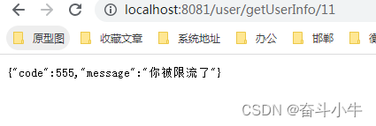
搭建网站七牛云CDN加速配置
打开七牛云后台;添加域名; 添加需要加速的域名,比如我添加的是motoshare.cn 源站配置,这里要用IP地址,访问的目录下面要有能访问测试的文件,尽量不要用源站域名,这个只能用加速二级域名&#x…...

算法|每日一题|做菜顺序|贪心
1402. 做菜顺序 原题地址: 力扣每日一题:做菜顺序 一个厨师收集了他 n 道菜的满意程度 satisfaction ,这个厨师做出每道菜的时间都是 1 单位时间。 一道菜的 「 like-time 系数 」定义为烹饪这道菜结束的时间(包含之前每道菜所花…...
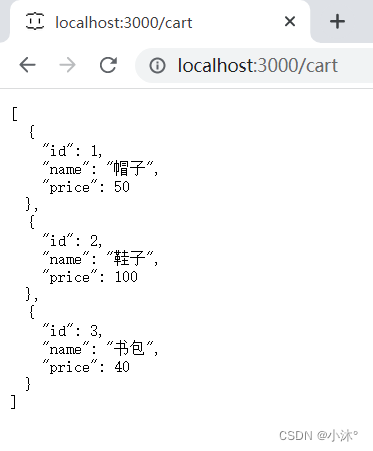
json-server工具准备后端接口服务环境
1.安装全局工具json-server(全局工具仅需要安装一次) 官网:json-server - npm 点击Getting started可以查看使用方法 在终端中输入yarn global add json-server或npm i json-server -g 如果输入json-server -v报错 再输入npm install -g j…...

AI写专著高效之道:AI专著生成工具,20万字专著快速搞定
学术专著写作与AI工具应用 学术专著的主要价值在于其内容的条理清晰和逻辑严谨,但这一点在写作过程中常常是最大的挑战。与专注于单一话题的期刊论文不同,专著的撰写需要构建一个包括绪论、理论基础、核心研究、应用拓展及结论的完整体系。每个章节都应…...

CardEditor:桌游设计师的批处理卡牌生成神器,让创意批量落地
CardEditor:桌游设计师的批处理卡牌生成神器,让创意批量落地 【免费下载链接】CardEditor 一款专为桌游设计师开发的批处理数值填入卡牌生成器/A card batch generator specially developed for board game designers 项目地址: https://gitcode.com/g…...

LaserGRBL:如何用开源软件实现专业级激光雕刻控制
LaserGRBL:如何用开源软件实现专业级激光雕刻控制 【免费下载链接】LaserGRBL Laser optimized GUI for GRBL 项目地址: https://gitcode.com/gh_mirrors/la/LaserGRBL LaserGRBL是一款专为激光雕刻和切割优化的GRBL控制器Windows图形界面软件,为…...

融合柯西变异与动态权重的蝴蝶优化算法性能跃迁
1. 蝴蝶优化算法的瓶颈与突破方向 蝴蝶优化算法(BOA)作为一种模拟自然界蝴蝶觅食行为的群体智能算法,自提出以来就在工程优化、机器学习参数调优等领域展现出独特优势。但我在实际使用中发现,传统BOA存在两个明显短板:一是容易陷入局部最优解…...

不止于定位:用微信小程序map组件打造一个简易门店导航与信息展示工具
从零构建门店导航小程序:map组件的商业级实践 每次走进陌生的商圈,我们总会下意识打开手机地图寻找目标店铺。这种基于地理位置的服务(LBS)已经成为现代商业的基础设施。作为小程序开发者,如何快速实现一个具备门店导航…...

Mermaid Live Editor:解决技术文档图表制作的5个核心痛点
Mermaid Live Editor:解决技术文档图表制作的5个核心痛点 【免费下载链接】mermaid-live-editor Edit, preview and share mermaid charts/diagrams. New implementation of the live editor. 项目地址: https://gitcode.com/GitHub_Trending/me/mermaid-live-edi…...

glogg实战指南:跨平台高效日志分析解决方案深度解析
glogg实战指南:跨平台高效日志分析解决方案深度解析 【免费下载链接】glogg A fast, advanced log explorer. 项目地址: https://gitcode.com/gh_mirrors/gl/glogg 面对海量日志文件时,传统文本编辑器和命令行工具的局限性日益凸显:内…...

lora-scripts企业级应用:客服话术、营销文案定制训练实战解析
LoRA-Scripts企业级应用:客服话术、营销文案定制训练实战解析 1. 为什么企业需要定制化文本生成 在当今商业环境中,个性化沟通已成为品牌差异化的关键。传统客服话术和营销文案往往面临三大痛点: 模板化严重:千篇一律的回复难以…...

FanControl终极指南:5分钟搞定Windows风扇智能控制,告别噪音烦恼[特殊字符]
FanControl终极指南:5分钟搞定Windows风扇智能控制,告别噪音烦恼🔥 【免费下载链接】FanControl.Releases This is the release repository for Fan Control, a highly customizable fan controlling software for Windows. 项目地址: http…...

告别IO口焦虑:用74HC595驱动8x8点阵屏,51单片机也能玩转动态显示
告别IO口焦虑:用74HC595驱动8x8点阵屏,51单片机也能玩转动态显示 当你在面包板上搭建第一个流水灯时,74HC595可能只是让LED依次点亮的工具。但这款售价不到1元的芯片,其实藏着更强大的潜力——它能让你用51单片机的3个IO口&#x…...