时间序列聚类的直观方法
一、介绍
我们将使用轮廓分数和一些距离度量来执行时间序列聚类实验,同时利用直观的可视化,让我们看看下面的时间序列:
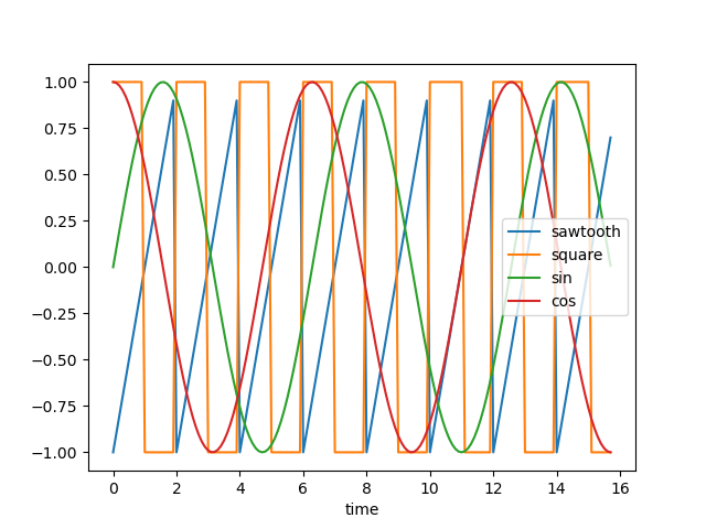
这些可以被视为具有正弦、余弦、方波和锯齿波的四种不同的周期性时间序列
如果我们添加随机噪声和距原点的距离来沿 y 轴移动序列并将它们随机化以使它们几乎难以辨别,则如下所示 - 现在很难将时间序列列分组为簇:

上面的图表是使用以下脚本创建的:
# Import necessary libraries
import os
import pandas as pd
import numpy as np# Import random module with an alias 'rand'
import random as rand
from scipy import signal# Import the matplotlib library for plotting
import matplotlib.pyplot as plt# Generate an array 'x' ranging from 0 to 5*pi with a step of 0.1
x = np.arange(0, 5*np.pi, 0.1)# Generate square, sawtooth, sin, and cos waves based on 'x'
y_square = signal.square(np.pi * x)
y_sawtooth = signal.sawtooth(np.pi * x)
y_sin = np.sin(x)
y_cos = np.cos(x)# Create a DataFrame 'df_waves' to store the waveforms
df_waves = pd.DataFrame([x, y_sawtooth, y_square, y_sin, y_cos]).transpose()# Rename the columns of the DataFrame for clarity
df_waves = df_waves.rename(columns={0: 'time',1: 'sawtooth',2: 'square',3: 'sin',4: 'cos'})# Plot the original waveforms against time
df_waves.plot(x='time', legend=False)
plt.show()# Add noise to the waveforms and plot them again
for col in df_waves.columns:if col != 'time':for i in range(1, 10):# Add noise to each waveform based on 'i' and a random valuedf_waves['{}_{}'.format(col, i)] = df_waves[col].apply(lambda x: x + i + rand.random() * 0.25 * i)# Plot the waveforms with added noise against time
df_waves.plot(x='time', legend=False)
plt.show()
二、问题陈述
现在我们需要决定聚类的基础。可能有两种方法:
- 我们希望将更接近一组的波形分组——欧氏距离较低的波形将被组合在一起。
- 我们想要对看起来相似的波形进行分组 - 它们具有相似的形状,但欧氏距离可能不低
2.1 距离度量
一般来说,我们希望根据形状 (2) 对时间序列进行分组,对于这样的聚类,我们可能希望使用距离度量,例如相关性,它们或多或少独立于波形的线性移位。
让我们检查一下具有上述定义的噪声的波形对之间的欧氏距离和相关性的热图:
使用欧几里德距离对波形进行分组很困难,因为我们可以看到任何波形对组中的模式都保持相似,例如平方和余弦之间的相关形状与平方和平方非常相似,除了对角线元素之外
我们可以看到,使用相关热图可以轻松地将所有形状组合在一起 - 因为相似的波形具有非常高的相关性(sin-sin 对),而 sin 和 cos 等对的相关性几乎为零。
2.2 剪影分数
分析上面显示的热图并根据高相关性分配组看起来是一个好主意,但是我们如何定义相关性阈值,高于该阈值我们应该对时间序列进行分组。看起来像是一个迭代过程,容易出现错误并且需要大量的手动工作。
在这种情况下,我们可以利用 Silhouette Score 为执行的聚类分配一个分数。我们的目标是最大化剪影得分。Silhouette 分数是如何工作的——尽管这可能需要单独讨论——让我们回顾一下高级定义
- 轮廓得分计算:单个数据点的轮廓得分是通过将其与其自身簇中的点的相似度(称为“a”的度量)与其与该点不属于的最近簇中的点的相似度进行比较来计算的(称为“b”的措施)。该点的轮廓得分由 (b — a) / max(a, b) 给出。
- a(内聚性):衡量该点与其自身簇中其他点的相似程度。较高的“a”表示该点在其簇内的位置很好。
- b(分离):测量点与最近邻簇中的点的不同程度。较低的“b”表示该点远离最近簇中的点。
- 轮廓分数的范围从 -1 到 1,其中高值(接近 1)表示该点聚类良好,低值(接近 -1)表示该点可能位于错误的聚类中。
2.解读剪影分数:
- 所有点的平均轮廓得分较高(接近 1)表明聚类定义明确且不同。
- 较低或负的平均轮廓分数(接近 -1)表明重叠或形成不良的簇。
- 0 左右的分数表示该点位于两个簇之间的边界上。
2.3 聚类
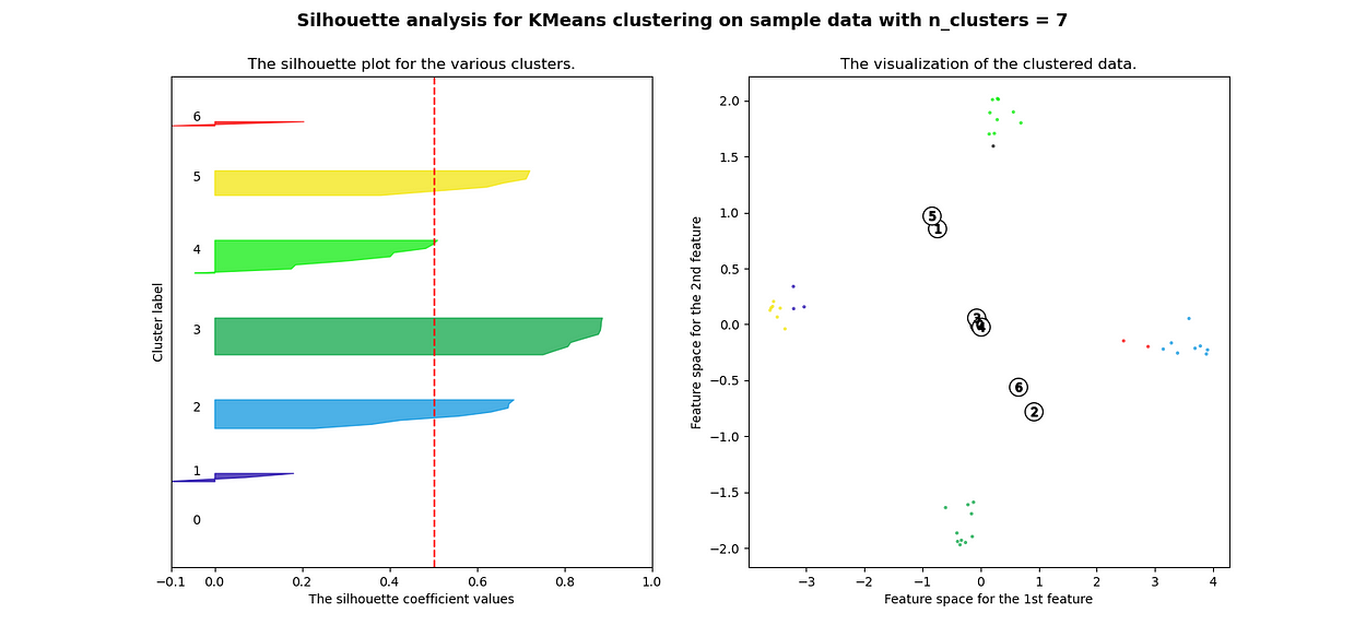
现在让我们利用上面计算的两个版本的距离度量,并尝试在利用 Silhouette 分数的同时对时间序列进行分组。测试结果更容易,因为我们已经知道存在四种不同的波形,因此理想情况下应该有四个簇。
欧氏距离
############ reduing components on eucl distance metrics for visualisation #######
pca = decomposition.PCA(n_components=2)
pca.fit(df_man_dist_euc)
df_fc_cleaned_reduced_euc = pd.DataFrame(pca.transform(df_man_dist_euc).transpose(), index = ['PC_1','PC_2'],columns = df_man_dist_euc.transpose().columns)index = 0
range_n_clusters = [2, 3, 4, 5, 6, 7, 8]# Iterate over different cluster numbers
for n_clusters in range_n_clusters:# Create a subplot with silhouette plot and cluster visualizationfig, (ax1, ax2) = plt.subplots(1, 2)fig.set_size_inches(15, 7)# Set the x and y axis limits for the silhouette plotax1.set_xlim([-0.1, 1])ax1.set_ylim([0, len(df_man_dist_euc) + (n_clusters + 1) * 10])# Initialize the KMeans clusterer with n_clusters and random seedclusterer = KMeans(n_clusters=n_clusters, n_init="auto", random_state=10)cluster_labels = clusterer.fit_predict(df_man_dist_euc)# Calculate silhouette score for the current cluster configurationsilhouette_avg = silhouette_score(df_man_dist_euc, cluster_labels)print("For n_clusters =", n_clusters, "The average silhouette_score is :", silhouette_avg)sil_score_results.loc[index, ['number_of_clusters', 'Euclidean']] = [n_clusters, silhouette_avg]index += 1# Calculate silhouette values for each samplesample_silhouette_values = silhouette_samples(df_man_dist_euc, cluster_labels)y_lower = 10# Plot the silhouette plotfor i in range(n_clusters):# Aggregate silhouette scores for samples in the cluster and sort themith_cluster_silhouette_values = sample_silhouette_values[cluster_labels == i]ith_cluster_silhouette_values.sort()# Set the y_upper value for the silhouette plotsize_cluster_i = ith_cluster_silhouette_values.shape[0]y_upper = y_lower + size_cluster_icolor = cm.nipy_spectral(float(i) / n_clusters)# Fill silhouette plot for the current clusterax1.fill_betweenx(np.arange(y_lower, y_upper), 0, ith_cluster_silhouette_values, facecolor=color, edgecolor=color, alpha=0.7)# Label the silhouette plot with cluster numbersax1.text(-0.05, y_lower + 0.5 * size_cluster_i, str(i))y_lower = y_upper + 10  # Update y_lower for the next plot# Set labels and title for the silhouette plotax1.set_title("The silhouette plot for the various clusters.")ax1.set_xlabel("The silhouette coefficient values")ax1.set_ylabel("Cluster label")# Add vertical line for the average silhouette scoreax1.axvline(x=silhouette_avg, color="red", linestyle="--")ax1.set_yticks([])  # Clear the yaxis labels / ticksax1.set_xticks([-0.1, 0, 0.2, 0.4, 0.6, 0.8, 1])# Plot the actual clusterscolors = cm.nipy_spectral(cluster_labels.astype(float) / n_clusters)ax2.scatter(df_fc_cleaned_reduced_euc.transpose().iloc[:, 0], df_fc_cleaned_reduced_euc.transpose().iloc[:, 1],marker=".", s=30, lw=0, alpha=0.7, c=colors, edgecolor="k")# Label the clusters and cluster centerscenters = clusterer.cluster_centers_ax2.scatter(centers[:, 0], centers[:, 1], marker="o", c="white", alpha=1, s=200, edgecolor="k")for i, c in enumerate(centers):ax2.scatter(c[0], c[1], marker="$%d$" % i, alpha=1, s=50, edgecolor="k")# Set labels and title for the cluster visualizationax2.set_title("The visualization of the clustered data.")ax2.set_xlabel("Feature space for the 1st feature")ax2.set_ylabel("Feature space for the 2nd feature")# Set the super title for the whole plotplt.suptitle("Silhouette analysis for KMeans clustering on sample data with n_clusters = %d" % n_clusters,fontsize=14, fontweight="bold")plt.savefig('sil_score_eucl.png')
plt.show()


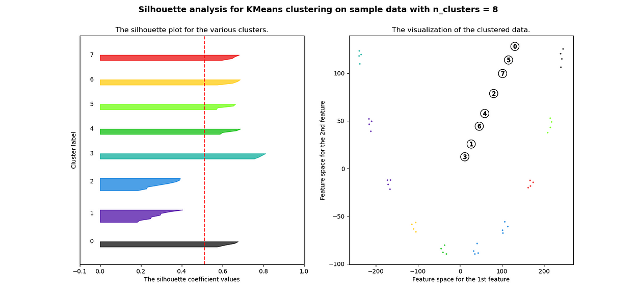
很明显,簇都是混合在一起的,并且不能为任何数量的簇提供良好的轮廓分数。这符合我们基于欧几里得距离热图的初步评估的预期
三、相关性
############ reduing components on eucl distance metrics for visualisation #######
pca = decomposition.PCA(n_components=2)
pca.fit(df_man_dist_corr)
df_fc_cleaned_reduced_corr = pd.DataFrame(pca.transform(df_man_dist_corr).transpose(), index = ['PC_1','PC_2'],columns = df_man_dist_corr.transpose().columns)index=0
range_n_clusters = [2,3,4,5,6,7,8]
for n_clusters in range_n_clusters:# Create a subplot with 1 row and 2 columnsfig, (ax1, ax2) = plt.subplots(1, 2)fig.set_size_inches(15, 7)# The 1st subplot is the silhouette plot# The silhouette coefficient can range from -1, 1 but in this example all# lie within [-0.1, 1]ax1.set_xlim([-0.1, 1])# The (n_clusters+1)*10 is for inserting blank space between silhouette# plots of individual clusters, to demarcate them clearly.ax1.set_ylim([0, len(df_man_dist_corr) + (n_clusters + 1) * 10])# Initialize the clusterer with n_clusters value and a random generator# seed of 10 for reproducibility.clusterer = KMeans(n_clusters=n_clusters, n_init="auto", random_state=10)cluster_labels = clusterer.fit_predict(df_man_dist_corr)# The silhouette_score gives the average value for all the samples.# This gives a perspective into the density and separation of the formed# clusterssilhouette_avg = silhouette_score(df_man_dist_corr, cluster_labels)print("For n_clusters =",n_clusters,"The average silhouette_score is :",silhouette_avg,)sil_score_results.loc[index,['number_of_clusters','corrlidean']] = [n_clusters,silhouette_avg]index=index+1sample_silhouette_values = silhouette_samples(df_man_dist_corr, cluster_labels)y_lower = 10for i in range(n_clusters):# Aggregate the silhouette scores for samples belonging to# cluster i, and sort themith_cluster_silhouette_values = sample_silhouette_values[cluster_labels == i]ith_cluster_silhouette_values.sort()size_cluster_i = ith_cluster_silhouette_values.shape[0]y_upper = y_lower + size_cluster_icolor = cm.nipy_spectral(float(i) / n_clusters)ax1.fill_betweenx(np.arange(y_lower, y_upper),0,ith_cluster_silhouette_values,facecolor=color,edgecolor=color,alpha=0.7,)# Label the silhouette plots with their cluster numbers at the middleax1.text(-0.05, y_lower + 0.5 * size_cluster_i, str(i))# Compute the new y_lower for next ploty_lower = y_upper + 10  # 10 for the 0 samplesax1.set_title("The silhouette plot for the various clusters.")ax1.set_xlabel("The silhouette coefficient values")ax1.set_ylabel("Cluster label")# The vertical line for average silhouette score of all the valuesax1.axvline(x=silhouette_avg, color="red", linestyle="--")ax1.set_yticks([])  # Clear the yaxis labels / ticksax1.set_xticks([-0.1, 0, 0.2, 0.4, 0.6, 0.8, 1])# 2nd Plot showing the actual clusters formedcolors = cm.nipy_spectral(cluster_labels.astype(float) / n_clusters)ax2.scatter(df_fc_cleaned_reduced_corr.transpose().iloc[:, 0], df_fc_cleaned_reduced_corr.transpose().iloc[:, 1], marker=".", s=30, lw=0, alpha=0.7, c=colors, edgecolor="k")#     for i in range(len(df_fc_cleaned_cleaned_reduced.transpose().iloc[:, 0])):
#                         ax2.annotate(list(df_fc_cleaned_cleaned_reduced.transpose().index)[i],
#                                      (df_fc_cleaned_cleaned_reduced.transpose().iloc[:, 0][i],
#                                       df_fc_cleaned_cleaned_reduced.transpose().iloc[:, 1][i] + 0.2))# Labeling the clusterscenters = clusterer.cluster_centers_# Draw white circles at cluster centersax2.scatter(centers[:, 0],centers[:, 1],marker="o",c="white",alpha=1,s=200,edgecolor="k",)for i, c in enumerate(centers):ax2.scatter(c[0], c[1], marker="$%d$" % i, alpha=1, s=50, edgecolor="k")ax2.set_title("The visualization of the clustered data.")ax2.set_xlabel("Feature space for the 1st feature")ax2.set_ylabel("Feature space for the 2nd feature")plt.suptitle("Silhouette analysis for KMeans clustering on sample data with n_clusters = %d"% n_clusters,fontsize=14,fontweight="bold",)plt.show()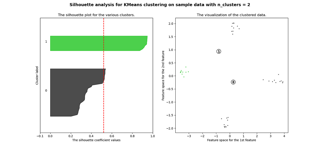

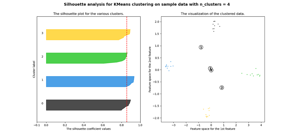


当选择的簇数为 4 时,我们可以看到清晰分离的簇,并且结果通常比欧几里德距离好得多。
欧氏距离和相关轮廓分数之间的比较
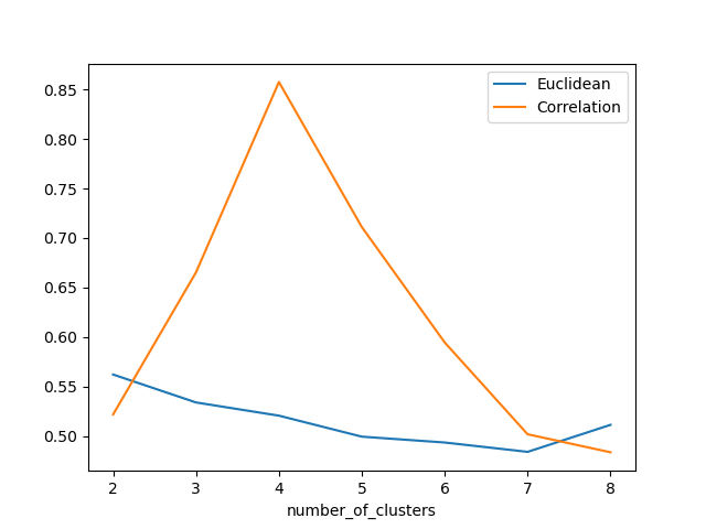
Silhouette 分数表示,当簇数为 4 时,基于相关性的距离矩阵提供最佳结果,而在欧几里德距离的情况下,其效果并不那么清晰
四、结论
在本文中,我们研究了如何使用欧几里德距离和相关性度量来执行时间序列聚类,并且我们还观察了这两种情况下结果的变化。如果我们在评估聚类时结合 Silhouette,我们可以使聚类步骤更加客观,因为它提供了一种很好的直观方法来查看聚类的分离程度。
参考
- https://scikit-learn.org [KMeans 和 Silhouette 分数]
- Plotly: Low-Code Data App Development [可视化库]
- https://scipy.org [用于创建信号数据]
-
吉里什·戴夫·库马尔·乔拉西亚·
如果您觉得我的讲解对您有帮助,请关注我以获取更多内容!如果您有任何问题或建议,请随时发表评论。
相关文章:
时间序列聚类的直观方法
一、介绍 我们将使用轮廓分数和一些距离度量来执行时间序列聚类实验,同时利用直观的可视化,让我们看看下面的时间序列: 这些可以被视为具有正弦、余弦、方波和锯齿波的四种不同的周期性时间序列 如果我们添加随机噪声和距原点的距离来沿 y 轴…...

vue3的reactive源码解析
reactive源码解析 总结一句: reactive是个函数。reactive函数返回了一个createReactiveObject函数,createReactiveObject又返回了一个“经new Proxy实例化”的对象。 详细介绍: 我们使用时传给reactive函数一个对象类型target,reactive又将target传给cr…...

【ElasticSearch系列-04】ElasticSearch的聚合查询操作
ElasticSearch系列整体栏目 内容链接地址【一】ElasticSearch下载和安装https://zhenghuisheng.blog.csdn.net/article/details/129260827【二】ElasticSearch概念和基本操作https://blog.csdn.net/zhenghuishengq/article/details/134121631【三】ElasticSearch的高级查询Quer…...

Redisson初始
最近的自己,一直都在做些老年的技术,没有啥升级,自己也快麻木了,自己该怎么说,那必须行动起来啊!~来来,我们一起增长自己的内功 分布式锁的最强实现: Redisson 1.概念 在介绍之前,我们要知道这个Redisson是啥? 难道就是Redis的son?(我第一次就这么认为的哈哈!) 事实也的确如…...
【华为OD题库-018】AI面板识别-Java
题目 Al识别到面板上有N(1<N≤100)个指示灯,灯大小一样,任意两个之间无重叠。由于AI识别误差,每次识别到的指示灯位置可能有差异,以4个坐标值描述Al识别的指示灯的大小和位置(左上角x1,y1,右下角x2.y2)。请输出先行…...
[概述] 点云滤波器
拓扑结构 点云是一种三维数据,有几种方法可以描述其空间结构,以利于展开搜索 https://blog.csdn.net/weixin_45824067/article/details/131317939 KD树 头文件:pcl/kdtree/kdtree_flann.h 函数:pcl::KdTreeFLANN 作用:…...

[笔记] 汉字判断
参考博客:如果判断一个字符是西文字符还是中文字符 结论: 汉字转数字后,会占两位字符位,两位都是负数。 参考下面代码 输入:你 输出:01 #include<bits/stdc.h> using namespace std; int main() {cha…...
Android开发笔记(三)—Activity篇
活动组件Activity 启动和结束生命周期启动模式信息传递Intent显式Intent隐式Intent 向下一个Activity发送数据向上一个Activity返回数据 附加信息利用资源文件配置字符串利用元数据传递配置信息给应用页面注册快捷方式 启动和结束 (1)从当前页面跳到新页…...
nodejs+vue+python+php在线购票系统的设计与实现-毕业设计
伴随着信息时代的到来,以及不断发展起来的微电子技术,这些都为在线购票带来了很好的发展条件。同时,在线购票的范围不断增大,这就需要有一种既能使用又能使用的、便于使用的、便于使用的系统来对其进行管理。在目前这种大环境下&a…...
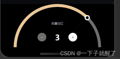
基于Taro + React 实现微信小程序半圆滑块组件、半圆进度条、弧形进度条、半圆滑行轨道(附源码)
效果: 功能点: 1、四个档位 2、可点击加减切换档位 3、可以点击区域切换档位 4、可以滑动切换档位 目的: 给大家提供一些实现思路,找了一圈,一些文章基本不能直接用,错漏百出,代码还藏着掖…...
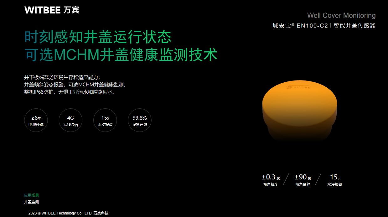
城市内涝解决方案:实时监测,提前预警,让城市更安全
城市内涝积水问题是指城市地区在短时间内遭遇强降雨后,地面积水过多,导致城市交通堵塞、居民生活不便、财产损失等问题。近年来,随着全球气候变化和城市化进程的加速,城市内涝积水问题越来越突出,成为城市发展中的一大…...

编译正点原子LINUXB报错make: arm-linux-gnueabihf-gcc:命令未找到
编译正点原子LINUX报错make: arm-linux-gnueabihf-gcc:命令未找到 1.报错内容2.解决办法3./bin/sh: 1: lzop: not found4.编译成功 1.报错内容 make: arm-linux-gnueabihf-gcc:命令未找到CHK include/config/kernel.releaseCHK include/generat…...
工地现场智慧管理信息化解决方案 智慧工地源码
智慧工地系统充分利用计算机技术、互联网、物联网、云计算、大数据等新一代信息技术,以PC端,移动端,设备端三位一体的管控方式为企业现场工程管理提供了先进的技术手段。让劳务、设备、物料、安全、环境、能源、资料、计划、质量、视频监控等…...
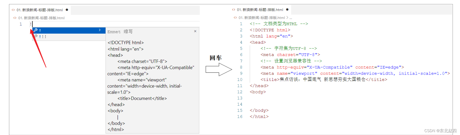
Javaweb之HTML,CSS的详细解析
2. HTML & CSS 1). 什么是HTML ? HTML: HyperText Markup Language,超文本标记语言。 超文本:超越了文本的限制,比普通文本更强大。除了文字信息,还可以定义图片、音频、视频等内容。 标记语言:由标签构成的语言…...
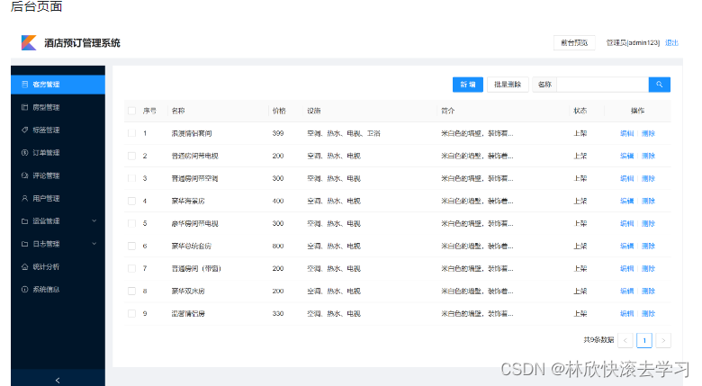
基于python+django+vue开发的酒店预订管理系统 - 毕业设计 - 课程设计
文章目录 源码下载地址项目介绍项目功能界面预览项目备注毕设定制,咨询 源码下载地址 点击这里下载源码 项目介绍 该系统是基于pythondjango开发的酒店预定管理系统。适用场景:大学生、课程作业、毕业设计。学习过程中,如遇问题可在github…...
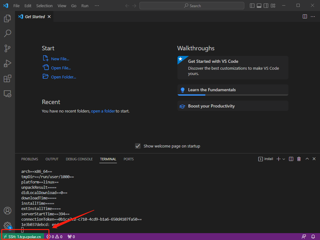
使用vscode实现远程开发,并通过内网穿透在公网环境下远程连接
文章目录 前言1、安装OpenSSH2、vscode配置ssh3. 局域网测试连接远程服务器4. 公网远程连接4.1 ubuntu安装cpolar内网穿透4.2 创建隧道映射4.3 测试公网远程连接 5. 配置固定TCP端口地址5.1 保留一个固定TCP端口地址5.2 配置固定TCP端口地址5.3 测试固定公网地址远程 前言 远程…...

ArrayList集合2
ArrayList集合的一些方法 ⑥chear()从列表中移除所有元素 ⑦.isEmpty()判断列表中是否包含元素,不包含返回true,否则返回false public class Test{public static void main(String[] args){Arraylist<String> list new Arraylist<String>()…...
vue+asp.net Web api前后端分离项目发布部署
一、前后端项目介绍 1.前端项目是使用vue脚手架进行创建的。 脚手架版本:vue/cli 5.0.8 编译器版本:vs code 1.82.2 2.后端是一个asp.net Core Web API 项目 后端框架版本:.NET 6.0 编译器版本:vs 2022 二、发布部署步骤 第…...
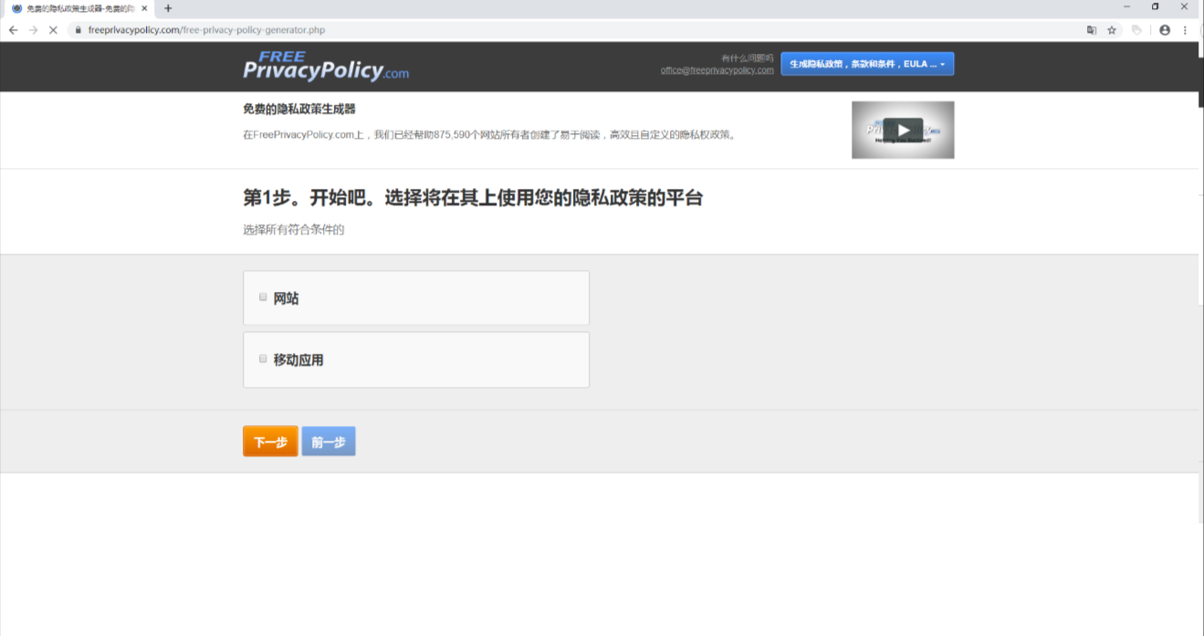
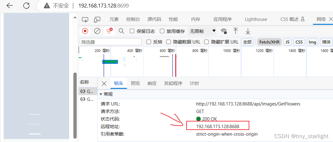
iOS App Store上传项目报错 缺少隐私政策网址(URL)解决方法
iOS App Store上传项目报错 缺少隐私政策网址(URL)解决方法 一、问题如下图所示: 二、解决办法:使用Google浏览器(翻译成中文)直接打开该网址 https://www.freeprivacypolicy.com/free-privacy-policy-generator.php 按…...

如何使用Ruby 多线程爬取数据
现在比较主流的爬虫应该是用python,之前也写了很多关于python的文章。今天在这里我们主要说说ruby。我觉得ruby也是ok的,我试试看写了一个爬虫的小程序,并作出相应的解析。 Ruby中实现网页抓取,一般用的是mechanize,使…...

软件测试从思维到实战:测试设计黄金法则与黑盒/灰盒/白盒全解析
📌为什么你的测试用例找不到Bug?你是否遇到过这样的场景:辛辛苦苦写了几十个测试用例,执行完发现一切正常,信心满满地发布上线。结果用户一用,马上就发现了严重问题。问题出在哪里?不是你的执行…...

m4s-converter:一键解决B站缓存视频的格式兼容难题
m4s-converter:一键解决B站缓存视频的格式兼容难题 【免费下载链接】m4s-converter 一个跨平台小工具,将bilibili缓存的m4s格式音视频文件合并成mp4 项目地址: https://gitcode.com/gh_mirrors/m4/m4s-converter 你是否曾经遇到过这样的场景&…...

ESJsonFormat-Xcode泛型支持:Xcode 7及以上版本的优化特性
ESJsonFormat-Xcode泛型支持:Xcode 7及以上版本的优化特性 【免费下载链接】ESJsonFormat-Xcode 将JSON格式化输出为模型的属性 项目地址: https://gitcode.com/gh_mirrors/es/ESJsonFormat-Xcode 如果你是一位iOS开发者,那么你一定遇到过将JSON数…...

手把手拆解FD-SOI工艺流程:从SOI衬底到应变硅外延的保姆级图解
从SOI衬底到应变硅外延:FD-SOI工艺全流程拆解指南 想象一下建造一座微型城市,每一栋建筑只有头发丝直径的万分之一大小。这就是FD-SOI工艺工程师的日常工作——在硅片上用原子级精度"建造"晶体管。与传统的体硅工艺不同,FD-SOI&…...

探索商业成功的奥秘:BABOK Guide v3深度解析
探索商业成功的奥秘:BABOK Guide v3深度解析 【下载地址】商业分析知识体系指南BABOKGuidev3 《商业分析知识体系指南(BABOK Guide v3)》是业界权威的商业分析专业标准,深受全球专业人士的认可与信赖。本指南经过严密的共识驱动开…...

【免费下载】 摩擦磨损仿真Archard模型 - FORTRAN子程序中文注释版:加速您的科研与工程项目
摩擦磨损仿真Archard模型 - FORTRAN子程序中文注释版:加速您的科研与工程项目 【下载地址】摩擦磨损仿真archard模型-FORTRAN子程序中文注释版 本仓库提供了一款专为摩擦磨损分析设计的Umeshmotion子程序模型,采用经典的Archard模型实现。此资源针对工程…...

CVBS转BT656/BT601,能成熟、应用广泛的低功耗视频解码器
GM7150是一款低功耗、9位NTSC/PAL视频解码器,由成都振芯科技股份有限公司生产。该芯片采用CMOS工艺,通过IC总线与PC或DSP相连构成应用系统。它内部包含1个模拟处理通道,能实现CVBS、S-Video视频信号源选择、A/D转换、自动钳位、自动增益控制(…...

【SysBench】从零到一:在Linux上部署sysbench-1.20进行数据库压测
1. 为什么你需要sysbench? 如果你正在使用MySQL或PostgreSQL这类数据库,迟早会遇到一个灵魂拷问:我的数据库到底能扛住多少并发请求?这时候sysbench就该登场了。这个工具就像数据库的"体能测试仪",能模拟真实…...

ContextMenuManager:5分钟掌握Windows右键菜单管理的终极免费方案
ContextMenuManager:5分钟掌握Windows右键菜单管理的终极免费方案 【免费下载链接】ContextMenuManager 🖱️ 纯粹的Windows右键菜单管理程序 项目地址: https://gitcode.com/gh_mirrors/co/ContextMenuManager 你是否厌倦了每次右键点击文件时&a…...

神经网络分子动力学与长程静电相互作用优化技术
1. 神经网络分子动力学与长程静电相互作用优化概述分子动力学模拟作为计算化学和材料科学的核心工具,其精度和效率直接决定了研究的深度和广度。传统分子动力学依赖经验力场,虽然计算速度快,但难以准确描述化学键断裂/形成等过程。而基于量子…...