【OpenCV实现图像:用OpenCV图像处理技巧之巧用直方图】
文章目录
- 概要
- 前置条件
- 统计数据分析
- 直方图均衡化原理
- 小结
概要
图像处理是计算机视觉领域中的重要组成部分,而直方图在图像处理中扮演着关键的角色。如何巧妙地运用OpenCV库中的图像处理技巧,特别是直方图相关的方法,来提高图像质量、改善细节以及调整曝光。
通过对图像的直方图进行分析和调整,能够优化图像的对比度、亮度和色彩平衡,从而使图像更具可视化效果。
直方图是一种统计图,用于表示图像中像素灰度级别的分布情况。在OpenCV中,可以使用直方图来了解图像的整体亮度分布,从而为后续处理提供基础。
OpenCV库中的函数,如cv2.calcHist和cv2.equalizeHist等,对图像的直方图进行均衡化。直方图均衡化是一种有效的方法,通过重新分配像素的强度值,使图像的亮度分布更均匀,提高图像的对比度和细节。
直方图匹配的应用,通过将目标图像的直方图调整到参考图像的直方图,实现两者之间的色彩一致性。这在图像配准和合成中有广泛的应用,提高了图像处理的精度和效果。
在低光照条件下拍摄图像的处理技巧。通过分析图像的直方图,可以采取针对性的方法,提高低光照图像中物体的可见性,改善图像的细节,并校正曝光过度或曝光不足的问题。
前置条件
一般来说,通过合理利用一些直方图的技巧,可以用于提高低光照拍摄图像中物体的可见性,改善图像的细节,以及校正曝光过度或曝光不足的图像。
import numpy as np
import matplotlib.pyplot as plt
from skimage.color import rgb2gray
from skimage.exposure import histogram, cumulative_distribution
from skimage import filters
from skimage.color import rgb2hsv, rgb2gray, rgb2yuv
from skimage import color, exposure, transform
from skimage.exposure import histogram, cumulative_distributionfrom skimage.io import imread# Load the image & remove the alpha or opacity channel (transparency)
dark_image = imread('img.png')[:,:,:3]# Visualize the image
plt.figure(figsize=(10, 10))
plt.title('Original Image: Plasma Ball')
plt.imshow(dark_image)
plt.show()
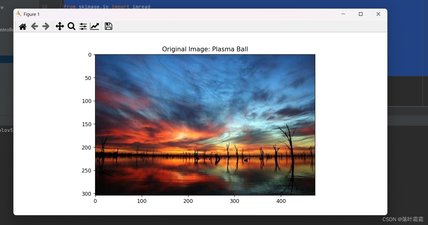
上述图像是在光照不足下进行拍摄的,接着我们就来通过控制直方图,来改善我们的视觉效果。
统计数据分析
使用以下代码:
def calc_color_overcast(image):# Calculate color overcast for each channelred_channel = image[:, :, 0]green_channel = image[:, :, 1]blue_channel = image[:, :, 2]# Create a dataframe to store the resultschannel_stats = pd.DataFrame(columns=['Mean', 'Std', 'Min', 'Median', 'P_80', 'P_90', 'P_99', 'Max'])# Compute and store the statistics for each color channelfor channel, name in zip([red_channel, green_channel, blue_channel], ['Red', 'Green', 'Blue']):mean = np.mean(channel)std = np.std(channel)minimum = np.min(channel)median = np.median(channel)p_80 = np.percentile(channel, 80)p_90 = np.percentile(channel, 90)p_99 = np.percentile(channel, 99)maximum = np.max(channel)channel_stats.loc[name] = [mean, std, minimum, median, p_80, p_90, p_99, maximum]return channel_stats
完整代码:
import numpy as np
import matplotlib.pyplot as plt
from skimage.color import rgb2gray
from skimage.exposure import histogram, cumulative_distribution
from skimage import filters
from skimage.color import rgb2hsv, rgb2gray, rgb2yuv
from skimage import color, exposure, transform
from skimage.exposure import histogram, cumulative_distribution
import pandas as pdfrom skimage.io import imread# Load the image & remove the alpha or opacity channel (transparency)
dark_image = imread('img.png')[:,:,:3]# Visualize the image
plt.figure(figsize=(10, 10))
plt.title('Original Image: Plasma Ball')
plt.imshow(dark_image)
plt.show()def calc_color_overcast(image):# Calculate color overcast for each channelred_channel = image[:, :, 0]green_channel = image[:, :, 1]blue_channel = image[:, :, 2]# Create a dataframe to store the resultschannel_stats = pd.DataFrame(columns=['Mean', 'Std', 'Min', 'Median','P_80', 'P_90', 'P_99', 'Max'])# Compute and store the statistics for each color channelfor channel, name in zip([red_channel, green_channel, blue_channel],['Red', 'Green', 'Blue']):mean = np.mean(channel)std = np.std(channel)minimum = np.min(channel)median = np.median(channel)p_80 = np.percentile(channel, 80)p_90 = np.percentile(channel, 90)p_99 = np.percentile(channel, 99)maximum = np.max(channel)channel_stats.loc[name] = [mean, std, minimum, median, p_80, p_90, p_99, maximum]return channel_stats
# 调用函数并传入图像
result_stats = calc_color_overcast(dark_image)# 打印结果
print(result_stats)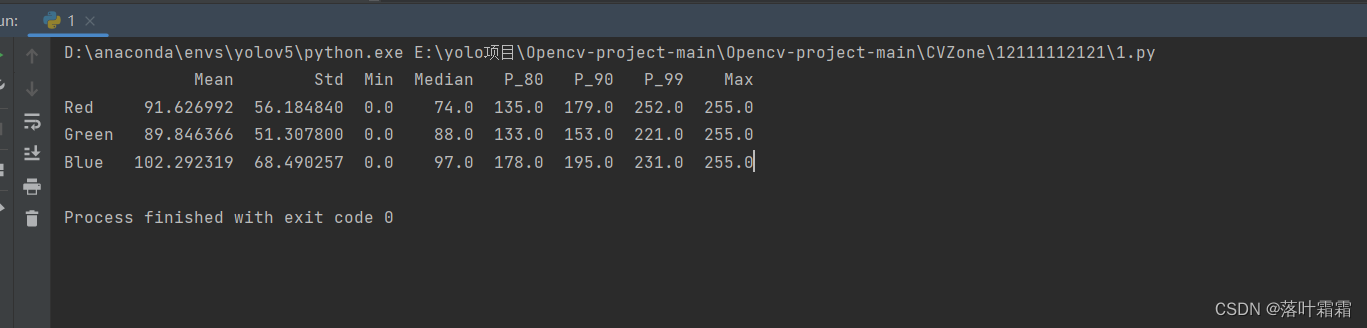
进而我们可以使用以下代码,来生成上述图像的直方图分布:
# Histogram plot
dark_image_intensity = img_as_ubyte(rgb2gray(dark_image))
freq, bins = histogram(dark_image_intensity)
plt.step(bins, freq*1.0/freq.sum())
plt.xlabel('intensity value')
plt.ylabel('fraction of pixels');
plt.show()  # 添加这一行以显示直方图
得到直方图可视化效果如下:
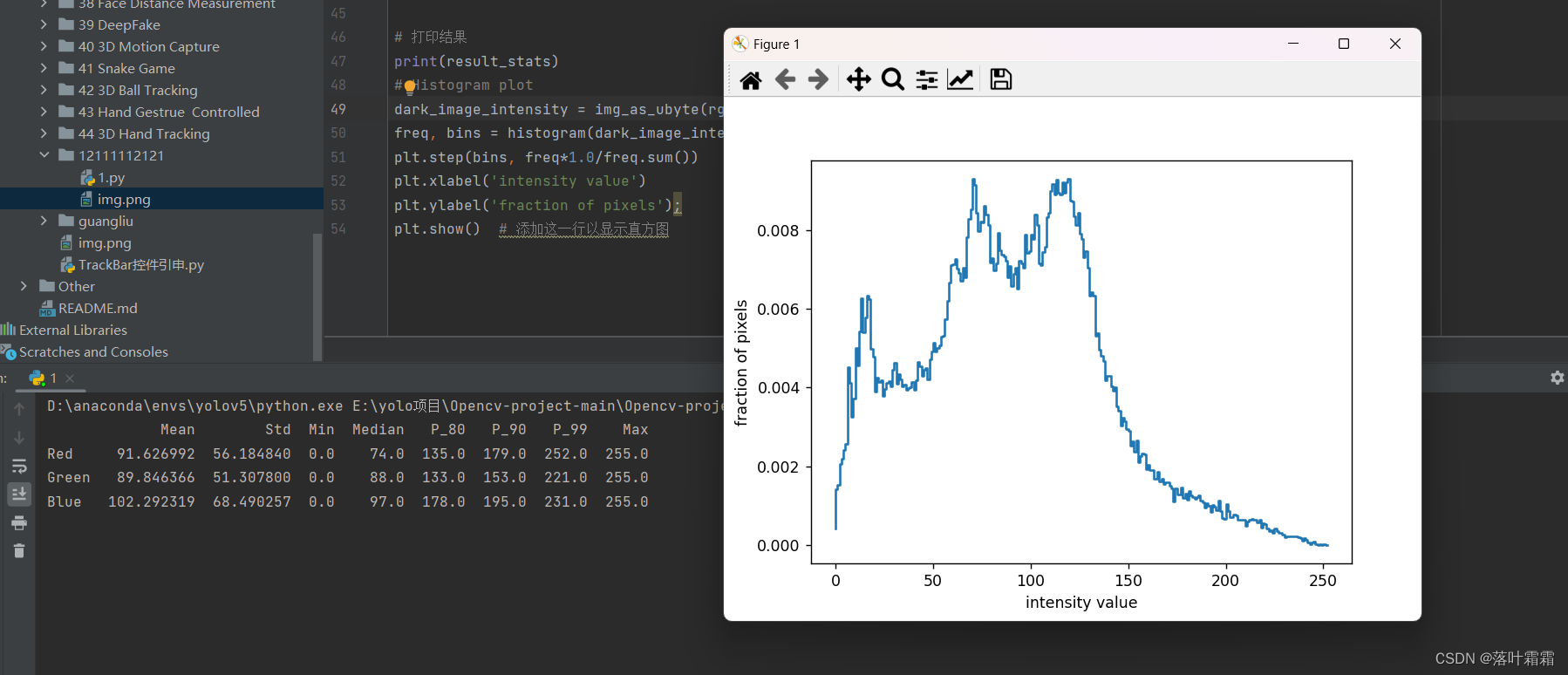
通过直方图的观察,可以注意到图像的像素平均强度似乎非常低,这进一步证实了图像的整体暗淡和曝光不足的情况。直方图展示了图像中像素强度值的分布情况,而大多数像素具有较低的强度值。这是有道理的,因为低像素强度值意味着图像中的大多数像素非常暗或呈现黑色。这样的观察有助于定量了解图像的亮度分布,为进一步的图像增强和调整提供了重要的线索。
直方图均衡化原理
直方图均衡化的基本原理是通过线性化图像的累积分布函数(CDF)来提高图像的对比度。实现这一目标的方法是将图像中每个像素的强度值映射到一个新的值,使得新的强度分布更加均匀。
可以通过以下几个步骤实现CDF的线性化:
将图像转换为灰度图:
如果图像不是灰度图,代码会将其转换为灰度图。这是因为直方图均衡化主要应用于灰度图。
计算累积分布函数(CDF):
通过计算图像像素的强度值的累积分布函数,可以了解每个强度值在图像中出现的累积频率。
绘制实际和目标CDF:
使用蓝色实线表示实际的CDF,使用红色实线表示目标CDF。目标CDF是一个线性分布,通过均匀分布来提高对比度。
绘制示例查找表:
绘制一个示例查找表,展示了像素强度值从原始值映射到目标值的过程。
自定义绘图:
对绘图进行自定义,包括设置坐标轴范围、标签和标题等。
import numpy as np
import matplotlib.pyplot as plt
from skimage.color import rgb2hsv, rgb2gray, rgb2yuv
from skimage.exposure import histogram, cumulative_distribution
import pandas as pd
from skimage import img_as_ubyte
from skimage.io import imread# Load the image & remove the alpha or opacity channel (transparency)
dark_image = imread('img.png')[:,:,:3]# Visualize the image
plt.figure(figsize=(10, 10))
plt.title('Original Image: Plasma Ball')
plt.imshow(dark_image)
plt.show()def calc_color_overcast(image):# Calculate color overcast for each channelred_channel = image[:, :, 0]green_channel = image[:, :, 1]blue_channel = image[:, :, 2]# Create a dataframe to store the resultschannel_stats = pd.DataFrame(columns=['Mean', 'Std', 'Min', 'Median','P_80', 'P_90', 'P_99', 'Max'])# Compute and store the statistics for each color channelfor channel, name in zip([red_channel, green_channel, blue_channel],['Red', 'Green', 'Blue']):mean = np.mean(channel)std = np.std(channel)minimum = np.min(channel)median = np.median(channel)p_80 = np.percentile(channel, 80)p_90 = np.percentile(channel, 90)p_99 = np.percentile(channel, 99)maximum = np.max(channel)channel_stats.loc[name] = [mean, std, minimum, median, p_80, p_90, p_99, maximum]return channel_statsdef plot_cdf(image):# Convert the image to grayscale if neededif len(image.shape) == 3:image = rgb2gray(image[:, :, :3])# Compute the cumulative distribution functionintensity = np.round(image * 255).astype(np.uint8)freq, bins = cumulative_distribution(intensity)# Plot the actual and target CDFstarget_bins = np.arange(256)target_freq = np.linspace(0, 1, len(target_bins))plt.step(bins, freq, c='b', label='Actual CDF')plt.plot(target_bins, target_freq, c='r', label='Target CDF')# Plot an example lookupexample_intensity = 50example_target = np.interp(freq[example_intensity], target_freq, target_bins)plt.plot([example_intensity, example_intensity, target_bins[-11], target_bins[-11]],[0, freq[example_intensity], freq[example_intensity], 0],'k--',label=f'Example lookup ({example_intensity} -> {example_target:.0f})')# Customize the plotplt.legend()plt.xlim(0, 255)plt.ylim(0, 1)plt.xlabel('Intensity Values')plt.ylabel('Cumulative Fraction of Pixels')plt.title('Cumulative Distribution Function')return freq, bins, target_freq, target_bins
# 调用函数并传入图像
result_stats = calc_color_overcast(dark_image)# 打印结果
print(result_stats)
# Histogram plot
# Histogram plot
dark_image_intensity = img_as_ubyte(rgb2gray(dark_image))
freq, bins = histogram(dark_image_intensity)
plt.step(bins, freq*1.0/freq.sum())
plt.xlabel('intensity value')
plt.ylabel('fraction of pixels')
plt.show()  # 添加这一行以显示直方图# 调用 plot_cdf 函数并传入图像
plot_cdf(dark_image)
plt.show()  # 添加这一行以显示CDF图形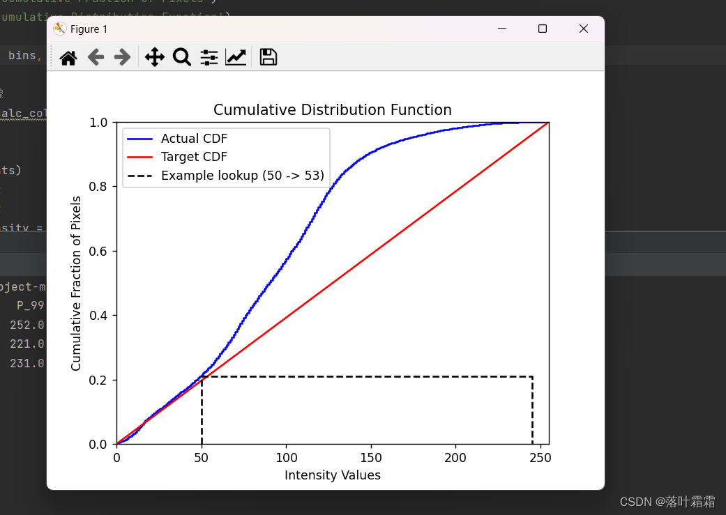
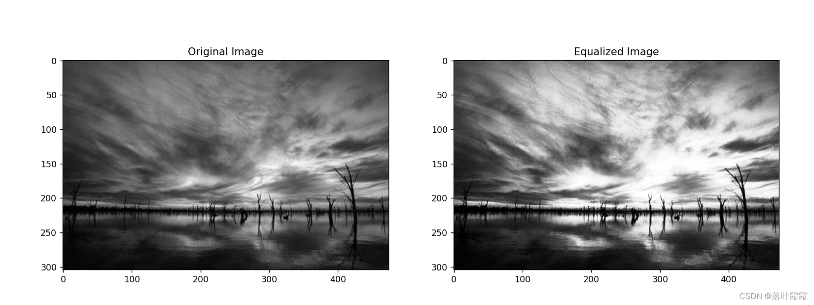
直方图均衡化实现结果:
import numpy as np
import matplotlib.pyplot as plt
from skimage.color import rgb2gray
from skimage.exposure import histogram, cumulative_distribution, equalize_hist
from skimage import img_as_ubyte
from skimage.io import imread# Load the image & remove the alpha or opacity channel (transparency)
dark_image = imread('img.png')[:,:,:3]# Visualize the original image
plt.figure(figsize=(10, 10))
plt.title('Original Image: Plasma Ball')
plt.imshow(dark_image)
plt.show()# Convert the image to grayscale
gray_image = rgb2gray(dark_image)# Apply histogram equalization
equalized_image = equalize_hist(gray_image)# Display the original and equalized images
plt.figure(figsize=(15, 7))
plt.subplot(1, 2, 1)
plt.title('Original Image')
plt.imshow(gray_image, cmap='gray')plt.subplot(1, 2, 2)
plt.title('Equalized Image')
plt.imshow(equalized_image, cmap='gray')plt.show()
扩展:
上面展示了最基本的直方图操作类型,接着让我们尝试不同类型的CDF技术,看看哪种技术适合给定的图像
# Linear
target_bins = np.arange(256)
# Sigmoid
def sigmoid_cdf(x, a=1):return (1 + np.tanh(a * x)) / 2
# Exponential
def exponential_cdf(x, alpha=1):return 1 - np.exp(-alpha * x)# Power
def power_law_cdf(x, alpha=1):return x ** alpha
# Other techniques:
def adaptive_histogram_equalization(image, clip_limit=0.03, tile_size=(8, 8)):clahe = exposure.equalize_adapthist(image, clip_limit=clip_limit, nbins=256, kernel_size=(tile_size[0], tile_size[1]))return clahe
def gamma_correction(image, gamma=1.0):corrected_image = exposure.adjust_gamma(image, gamma)return corrected_image
def contrast_stretching_percentile(image, lower_percentile=5, upper_percentile=95):in_range = tuple(np.percentile(image, (lower_percentile, upper_percentile)))stretched_image = exposure.rescale_intensity(image, in_range)return stretched_imagedef unsharp_masking(image, radius=5, amount=1.0):blurred_image = filters.gaussian(image, sigma=radius, multichannel=True)sharpened_image = (image + (image - blurred_image) * amount).clip(0, 1)return sharpened_imagedef equalize_hist_rgb(image):equalized_image = exposure.equalize_hist(image)return equalized_imagedef equalize_hist_hsv(image):hsv_image = color.rgb2hsv(image[:,:,:3])hsv_image[:, :, 2] = exposure.equalize_hist(hsv_image[:, :, 2])hsv_adjusted = color.hsv2rgb(hsv_image)return hsv_adjusteddef equalize_hist_yuv(image):yuv_image = color.rgb2yuv(image[:,:,:3])yuv_image[:, :, 0] = exposure.equalize_hist(yuv_image[:, :, 0])yuv_adjusted = color.yuv2rgb(yuv_image)return yuv_adjusted
使用代码:
import numpy as np
import matplotlib.pyplot as plt
from skimage.io import imread
from skimage.color import rgb2gray
from skimage.exposure import histogram, cumulative_distribution
from skimage import exposure, color, filters# Load the image & remove the alpha or opacity channel (transparency)
dark_image = imread('img.png')[:, :, :3]# Visualize the original image
plt.figure(figsize=(10, 10))
plt.title('Original Image: Plasma Ball')
plt.imshow(dark_image)
plt.show()# Linear
target_bins = np.arange(256)
# Sigmoid
def sigmoid_cdf(x, a=1):return (1 + np.tanh(a * x)) / 2
# Exponential
def exponential_cdf(x, alpha=1):return 1 - np.exp(-alpha * x)# Power
def power_law_cdf(x, alpha=1):return x ** alpha
# Other techniques:
def adaptive_histogram_equalization(image, clip_limit=0.03, tile_size=(8, 8)):clahe = exposure.equalize_adapthist(image, clip_limit=clip_limit, nbins=256, kernel_size=(tile_size[0], tile_size[1]))return clahe
def gamma_correction(image, gamma=1.0):corrected_image = exposure.adjust_gamma(image, gamma)return corrected_image
def contrast_stretching_percentile(image, lower_percentile=5, upper_percentile=95):in_range = tuple(np.percentile(image, (lower_percentile, upper_percentile)))stretched_image = exposure.rescale_intensity(image, in_range)return stretched_imagedef unsharp_masking(image, radius=5, amount=1.0):blurred_image = filters.gaussian(image, sigma=radius, multichannel=True)sharpened_image = (image + (image - blurred_image) * amount).clip(0, 1)return sharpened_imagedef equalize_hist_rgb(image):equalized_image = exposure.equalize_hist(image)return equalized_imagedef equalize_hist_hsv(image):hsv_image = color.rgb2hsv(image[:,:,:3])hsv_image[:, :, 2] = exposure.equalize_hist(hsv_image[:, :, 2])hsv_adjusted = color.hsv2rgb(hsv_image)return hsv_adjusteddef equalize_hist_yuv(image):yuv_image = color.rgb2yuv(image[:,:,:3])yuv_image[:, :, 0] = exposure.equalize_hist(yuv_image[:, :, 0])yuv_adjusted = color.yuv2rgb(yuv_image)return yuv_adjusted
def apply_cdf(image, cdf_function, *args, **kwargs):# Convert the image to grayscalegray_image = rgb2gray(image)# Calculate the cumulative distribution function (CDF)intensity = np.round(gray_image * 255).astype(np.uint8)cdf_values, bins = cumulative_distribution(intensity)# Apply the specified CDF functiontransformed_cdf = cdf_function(cdf_values, *args, **kwargs)# Map the CDF values back to intensity valuestransformed_intensity = np.interp(intensity, cdf_values, transformed_cdf)# Rescale the intensity values to [0, 1]transformed_intensity = transformed_intensity / 255.0# Apply the transformation to the original imagetransformed_image = image.copy()for i in range(3):transformed_image[:, :, i] = transformed_intensityreturn transformed_image# Apply and visualize different CDF techniques
linear_image = apply_cdf(dark_image, lambda x: x)
sigmoid_image = apply_cdf(dark_image, sigmoid_cdf, a=1)
exponential_image = apply_cdf(dark_image, exponential_cdf, alpha=1)
power_law_image = apply_cdf(dark_image, power_law_cdf, alpha=1)
adaptive_hist_eq_image = adaptive_histogram_equalization(dark_image)
gamma_correction_image = gamma_correction(dark_image, gamma=1.5)
contrast_stretch_image = contrast_stretching_percentile(dark_image)
unsharp_mask_image = unsharp_masking(dark_image)
equalized_hist_rgb_image = equalize_hist_rgb(dark_image)
equalized_hist_hsv_image = equalize_hist_hsv(dark_image)
equalized_hist_yuv_image = equalize_hist_yuv(dark_image)# Visualize the results
plt.figure(figsize=(15, 15))
plt.subplot(4, 4, 1), plt.imshow(linear_image), plt.title('Linear CDF')
plt.subplot(4, 4, 2), plt.imshow(sigmoid_image), plt.title('Sigmoid CDF')
plt.subplot(4, 4, 3), plt.imshow(exponential_image), plt.title('Exponential CDF')
plt.subplot(4, 4, 4), plt.imshow(power_law_image), plt.title('Power Law CDF')
plt.subplot(4, 4, 5), plt.imshow(adaptive_hist_eq_image), plt.title('Adaptive Histogram Equalization')
plt.subplot(4, 4, 6), plt.imshow(gamma_correction_image), plt.title('Gamma Correction')
plt.subplot(4, 4, 7), plt.imshow(contrast_stretch_image), plt.title('Contrast Stretching')
plt.subplot(4, 4, 8), plt.imshow(unsharp_mask_image), plt.title('Unsharp Masking')
plt.subplot(4, 4, 9), plt.imshow(equalized_hist_rgb_image), plt.title('Equalized Histogram (RGB)')
plt.subplot(4, 4, 10), plt.imshow(equalized_hist_hsv_image), plt.title('Equalized Histogram (HSV)')
plt.subplot(4, 4, 11), plt.imshow(equalized_hist_yuv_image), plt.title('Equalized Histogram (YUV)')plt.tight_layout()
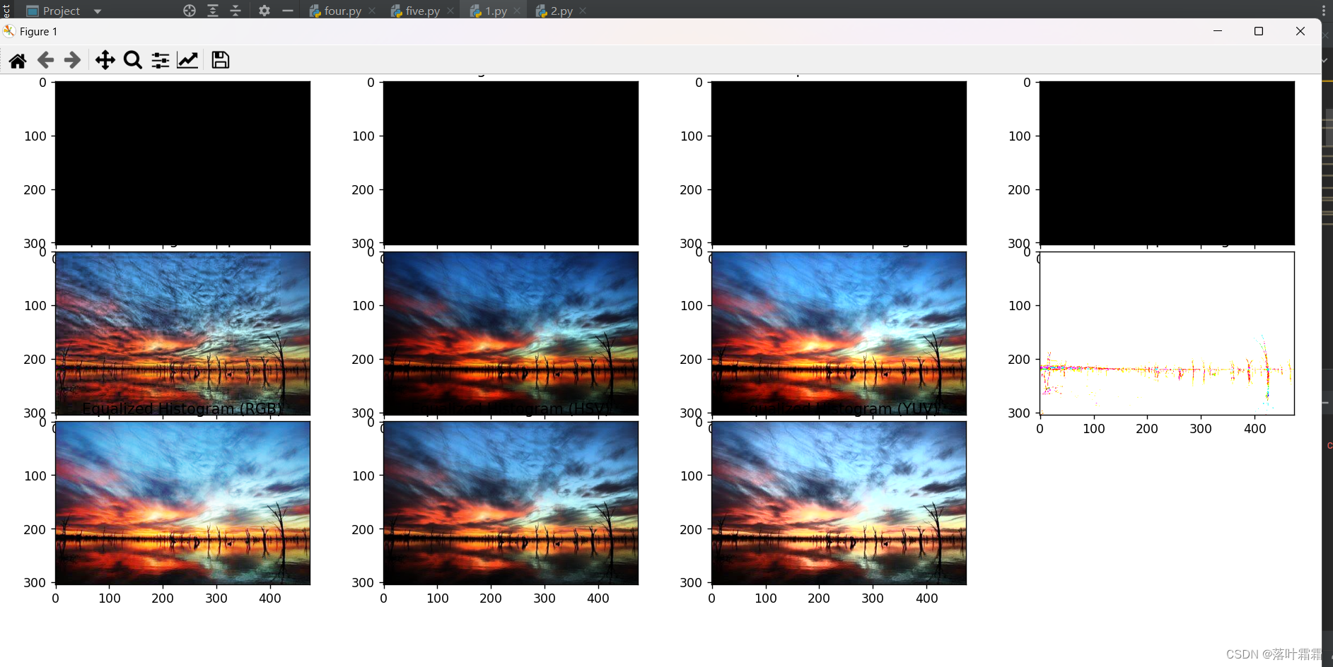
plt.show()输出结果:
小结
有多种方法和技术可用于改善RGB图像的可视效果,但其中许多方法都需要手动调整参数。上述输出展示了使用不同直方图操作生成的亮度校正效果。通过观察,发现HSV调整、指数变换、对比度拉伸和unsharp masking的效果都是令人满意的。
HSV调整:
HSV调整涉及将RGB图像转换为HSV颜色空间并修改强度分量。这种技术似乎在提高图像可视化效果方面取得了令人满意的结果。
指数变换:
指数变换用于根据指数函数调整像素强度。这种方法在提高图像整体亮度和视觉吸引力方面表现出色。
对比度拉伸:
对比度拉伸旨在通过拉伸指定百分位范围内的强度值来增强图像对比度。结果表明,这种技术有效地提高了图像的视觉质量。
Unsharp Masking:
Unsharp masking涉及通过减去模糊版本来创建图像的锐化版本。应用unsharp masking似乎增强了图像的细节和边缘
相关文章:
【OpenCV实现图像:用OpenCV图像处理技巧之巧用直方图】
文章目录 概要前置条件统计数据分析直方图均衡化原理小结 概要 图像处理是计算机视觉领域中的重要组成部分,而直方图在图像处理中扮演着关键的角色。如何巧妙地运用OpenCV库中的图像处理技巧,特别是直方图相关的方法,来提高图像质量、改善细…...

【Android】画面卡顿优化列表流畅度四之Glide几个常用参数设置
好像是一年前快两年了,笔者解析过glide的源码,也是因为觉得自己熟悉一些,也就没太关注过项目里glide的具体使用对当前业务的影响;主要是自负,还有就是真没有碰到过这样的数据加载情况。暴露了经验还是不太足够 有兴趣的…...

js控制手机蓝牙
要使用JavaScript控制手机蓝牙,您需要使用Web Bluetooth API。这是一种新的Web API,可以让Web应用程序访问和控制蓝牙设备。 以下是一些步骤,以便您开始使用Web Bluetooth API: 检查浏览器支持:首先,您需要…...
“)
C++11 原始字符串字面量R“()“
原始字符串字面量(Raw String Literals) R"()"是C11引入的一项特性,它允许创建不需要转义字符的字符串字面量。字符串中包含特殊字符、换行符和其他转义字符时,不需要反斜杠转义它们。 原始(Raw):不用使用反…...

【Vue原理解析】之虚拟DOM
Vue.js是一款流行的JavaScript框架,它采用了虚拟DOM(Virtual DOM)的概念来提高性能和开发效率。虚拟DOM是Vue.js的核心之一,它通过在内存中构建一个轻量级的DOM树来代替直接操作真实的DOM,从而减少了对真实DOM的操作次…...
HCIE-灾备技术和安全服务
灾备技术 灾备包含两个概念:容灾、备份 备份是为了保证数据的完整性,数据不丢失。全量备份、增量备份,备份数据还原。 容灾是为了保证业务的连续性,尽可能不断业务。 快照:保存的不是底层块数据,保存的是逻…...

【图论实战】Boost学习 01:基本操作
文章目录 头文件图的构建图的可视化基本操作 头文件 #include <boost/graph/adjacency_list.hpp> #include <boost/graph/graphviz.hpp> #include <boost/graph/properties.hpp> #include <boost/property_map/property_map.hpp> #include <boost/…...
Rust 中的引用与借用
目录 1、引用与借用 1.1 可变引用 1.2 悬垂引用 1.3 引用的规则 2、slice 类型 2.1 字符串字面量其实就是一个slice 2.2 总结 1、引用与借用 在之前我们将String 类型的值返回给调用函数,这样会导致这个String会被移动到函数中,这样在原来的作用域…...
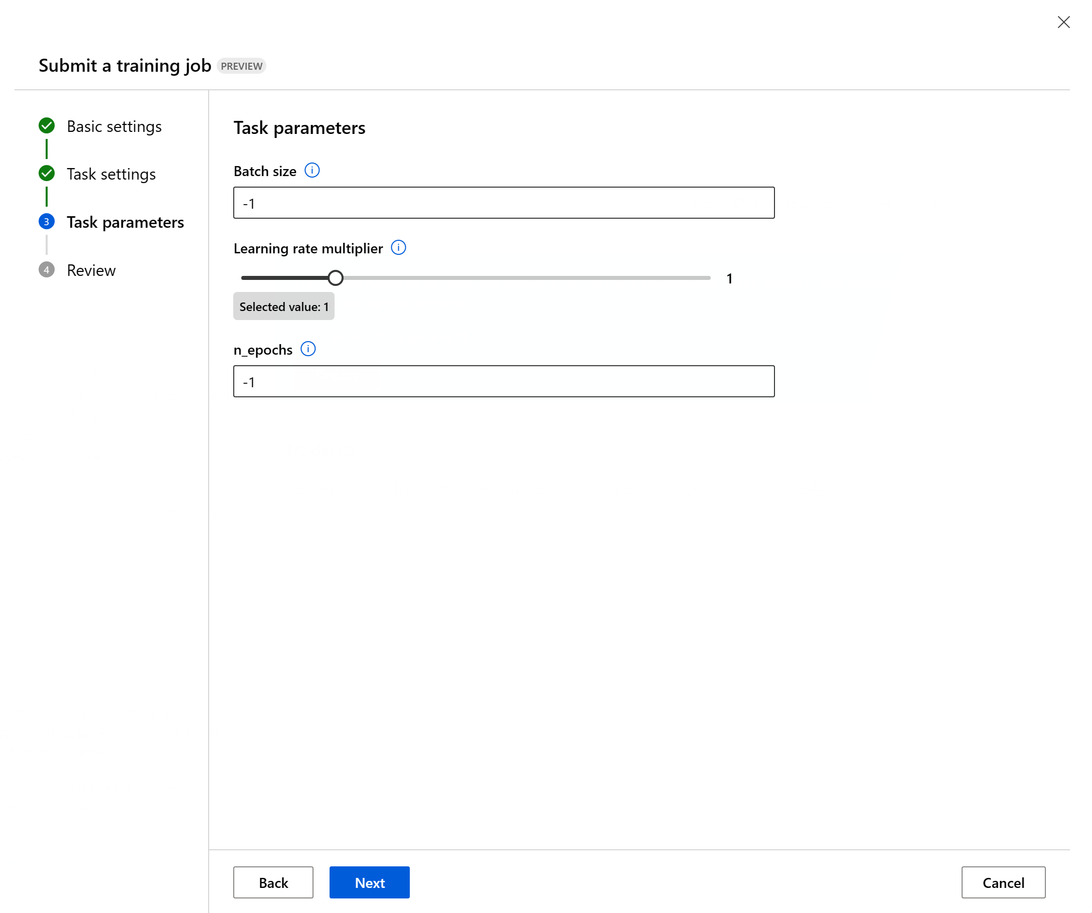
Azure 机器学习:在 Azure 机器学习中使用 Azure OpenAI 模型
目录 一、环境准备二、Azure 机器学习中的 OpenAI 模型是什么?三、在机器学习中访问 Azure OpenAI 模型连接到 Azure OpenAI部署 Azure OpenAI 模型 四、使用自己的训练数据微调 Azure OpenAI 模型使用工作室微调微调设置训练数据自定义微调参数部署微调的模型 使用…...
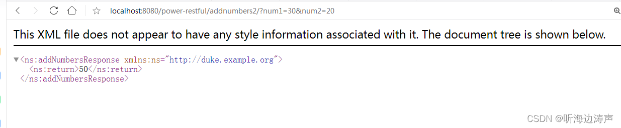
XML Web 服务 Eclipse实现中的sun-jaxws.xml文件
说明 在sun-jaxws.xml文件,可以配置endpoint、handler-chain等内容。在这个文件中配置的内容会覆盖在Java代码中使用注解属性配置的的内容。 这个文件根据自己的项目内容修改完成以后,作为web应用的一部分部署到web容器中(放到web应用的WEB…...
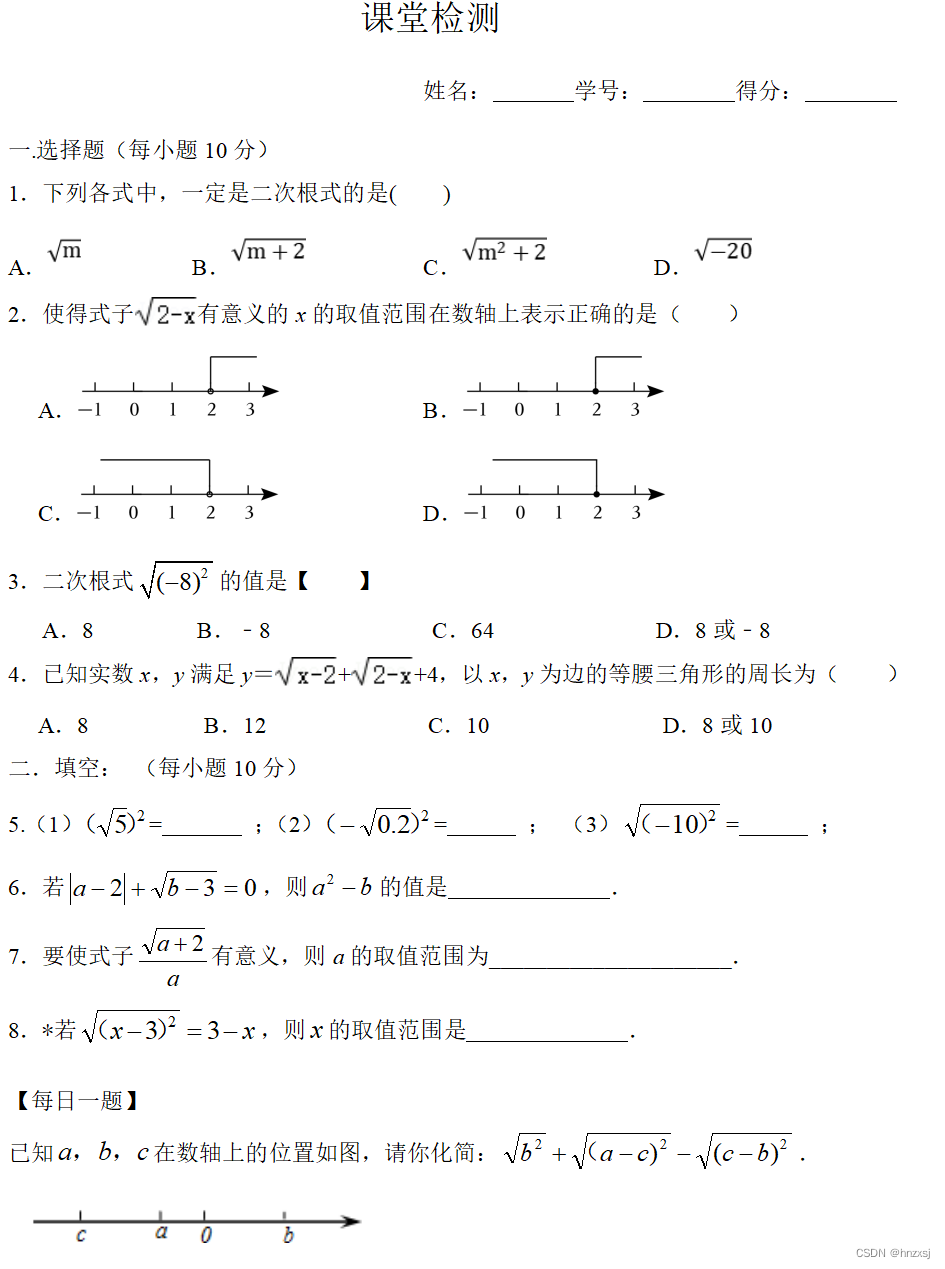
16.1 二次根式 教学设计及课堂检测设计
课堂检测如下:...

Android数据流的狂欢:Channel与Flow
在 Android 应用程序的开发中,处理异步数据流是一个常见的需求。为了更好地应对这些需求,Kotlin 协程引入了 Channel 和 Flow,它们提供了强大的工具来处理数据流,实现生产者-消费者模式,以及构建响应式应用程序。 本文…...

Java 单元测试最佳实践:如何充分利用测试自动化
单元测试是众所周知的做法,但还有很大的改进空间!在这篇文章中,我们讨论最有效的单元测试最佳实践,包括在此过程中最大化自动化工具的方法。我们还将讨论代码覆盖率、模拟依赖关系和整体测试策略。 什么是单元测试? 单…...
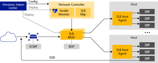
windows系统用于 SDN 的软件负载均衡器 (SLB)
适用于:Azure Stack HCI 版本 22H2 和 21H2;Windows Server 2022、Windows Server 2019、Windows Server 2016 软件负载均衡器包括哪些内容? 软件负载均衡器提供以下功能: 适用于北/南和东/西 TCP/UDP 流量的第 4 层 (L4) 负载均…...
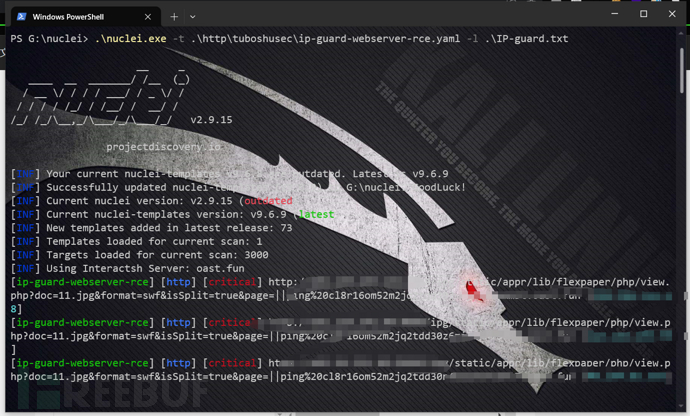
漏洞复现--IP-guard flexpaper RCE
免责声明: 文章中涉及的漏洞均已修复,敏感信息均已做打码处理,文章仅做经验分享用途,切勿当真,未授权的攻击属于非法行为!文章中敏感信息均已做多层打马处理。传播、利用本文章所提供的信息而造成的任何直…...
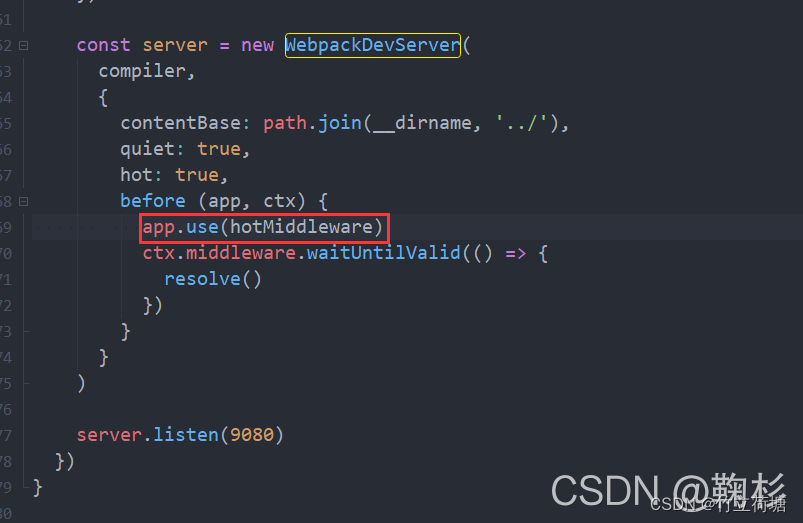
Electron-vue出现GET http://localhost:9080/__webpack_hmr net::ERR_ABORTED解决方案
GET http://localhost:9080/__webpack_hmr net::ERR_ABORTED解决方案 使用版本解决方案解决总结 使用版本 以下是我解决此问题时使用的electron和vue等的一些版本信息 【附】经过测试 electron 的版本为 13.1.4 时也能解决 解决方案 将项目下的 .electron-vue/dev-runner.js…...

Linux---(六)自动化构建工具 make/Makefile
文章目录 一、make/Makefile二、快速查看(1)建立Makefile文件(2)编辑Makefile文件(3)解释(4)效果展示 三、背后的基本知识、原理(1)如何清理对应的临时文件呢…...

谷歌:编写干净的代码以减少认知负荷
您是否曾经阅读过代码却发现很难理解?您可能正在经历认知负荷! 认知负荷是指完成一项任务所需的脑力劳动量。阅读代码时,您必须记住变量值、条件逻辑、循环索引、数据结构状态和接口契约等信息。随着代码变得更加复杂,认知负荷也…...
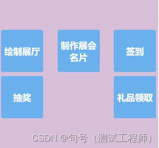
微信小程序display常用属性和子元素排列方式介绍
wxss中display常用显示属性与css一致,介绍如下: 针对元素本身显示的属性: displayblock,元素显示换行displayinline,元素显示换行,但不可设置固定的宽度和高度,也不可设置上下方向的margin和p…...
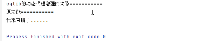
设计模式—结构型模式之代理模式
设计模式—结构型模式之代理模式 代理模式(Proxy Pattern) ,给某一个对象提供一个代理,并由代理对象控制对原对象的引用,对象结构型模式。 静态代理 比如我们有一个直播平台,提供了直播功能,但是如果不进行美颜,可能就比较冷清…...

Python基础语法:访问器@property和修改器@xxx.setter
一、简介 访问器和修改器也是装饰器的一种。 property: 访问器,getter xxx.setter: 修改器,setter 访问器和修改器的根本目的是想将属性私有化,提供getter&setter去访问。 访问器和修改器能够做到访问属性其实在调用getter方法࿰…...

C++中显示与隐式加载dll的使用与区别
一、什么是 DLL?DLL(Dynamic Link Library) 是 Windows 下的动态链接库,包含可被多个程序共享的函数、资源或类。使用 DLL 可以实现代码复用、模块化设计和插件机制。在 C 中,调用 DLL 中的函数有两种主要方式…...

用C语言解决‘换硬币’问题?我来教你如何调试和验证你的循环逻辑
用C语言解决‘换硬币’问题?我来教你如何调试和验证你的循环逻辑 当你第一次面对"换硬币"这类组合问题时,那种既兴奋又困惑的感觉我至今记忆犹新。作为C语言初学者,理解多重循环的运作机制就像在迷宫中寻找出口——每次你以为找到了…...

Wechat2RSS:微信公众号转RSS订阅工具
文章目录Wechat2RSS:微信公众号转RSS订阅工具Wechat2RSS:微信公众号转RSS订阅工具 ttttmr开源的Wechat2RSS项目,目前在GitHub上获得1409颗Star,项目地址为https://github.com/ttttmr/Wechat2RSS。该工具的核心作用是将微信公众号…...

PlayAI语音合成质量到底如何?12款竞品横向对比+5项MOS/LSD/STOI硬指标揭榜
更多请点击: https://kaifayun.com 第一章:PlayAI语音合成质量评测报告 PlayAI 是一款面向开发者与内容创作者的实时语音合成(TTS)服务,支持多语种、多音色及情感可控输出。本报告基于客观可复现的评测流程࿰…...

TVA注意力层INT8量化配置技巧
重磅预告:本专栏将独家连载系列丛书《智能体视觉技术与应用》部分精华内容,该书是世界首套系统阐述“因式智能体”视觉理论与实践的专著,特邀美国 TypeOne 公司首席科学家、斯坦福大学博士 Bohan 担任技术顾问。Bohan先生师从美国三院院士、“…...

Ubuntu经常安装软件
1、垃圾清理工具stacer sudo apt updatesudo apt install stacer apt cleanapt autocleanapt autoremove 2、类似与everything的工具Fsearcch 1sudo add-apt-repository ppa:christian-boxdoerfer/fsearch-stable 2sudo apt update 3sudo apt install fsearch (注…...

uWSGI目录穿越漏洞CVE-2018-7490深度利用与防御实战
1. 这不是“读文件”那么简单:uWSGI目录穿越在真实攻防链中的定位与误判代价你刚在Vulfocus靶场里跑通了CVE-2018-7490的PoC,用curl "http://target:8080/?p../../../../etc/passwd"成功读出了root:x:0:0:root:/root:/bin/bash,截…...

2026这6款神级降AIGC平台大公开,一键让AIGC率直逼绝对安全线!
步入 2026 年,学术圈的风向早已不是从前的模样。曾经大家还在为查重率发愁,如今却陷入了更棘手的困境——如何在不破坏论文专业性的前提下,彻底消除 AI 痕迹?随着 AIGC 检测技术不断进化,高校对论文的审核标准也愈发严…...

Python多智能体建模终极指南:用Mesa轻松构建复杂系统仿真
Python多智能体建模终极指南:用Mesa轻松构建复杂系统仿真 【免费下载链接】mesa Mesa is an open-source Python library for agent-based modeling, ideal for simulating complex systems and exploring emergent behaviors. 项目地址: https://gitcode.com/gh_…...