[足式机器人]Part4 南科大高等机器人控制课 CH12 Robotic Motion Control
本文仅供学习使用
本文参考:
B站:CLEAR_LAB
笔者带更新-运动学
课程主讲教师:
Prof. Wei Zhang
课程链接 :
https://www.wzhanglab.site/teaching/mee-5114-advanced-control-for-robotics/
南科大高等机器人控制课 Ch12 Robotic Motion Control
- 1. Basic Linear Control Design
- 1.1 Error Response
- 1.2 Standard Second-Order Systems
- 1.3 Second-Order Response Characteristics
- 1.4 State-Space Controller Design
- 2. Motion Control Problems
- 2.1 Robotic Motion Control Problem
- 2.2 Variations in Robot Motion Control
- 3. Motion Control with Velocity/Acceleration as Input
- 3.1 Velocity-Resolved Control
- 3.2.1 Velocity-Resolved Joint Space Control
- 3.2.2 Velocity-Resolved Task Space Control
- 3.2 Acceleration-Resolved Control
- 3.2.1 Acceleration-Resolved Control in Joint Space
- 3.2.2 Acceleration-Resolved Control in Task Space
- 4. Motion Control with Torque as Input and Task Space Inverse Dynamics
- 4.1 Recall Properties of Robot Dynamics
- 4.2 Computed Torque Control
- 4.3 Inverse Dynamics Control
机器人——运动能力、计算能力、感知决策能力 的机电系统
1. Basic Linear Control Design
1.1 Error Response

Steady-state error : e s s = lim t → ∞ θ e ( t ) e_{\mathrm{ss}}=\underset{t\rightarrow \infty}{\lim}\theta _{\mathrm{e}}\left( t \right) ess=t→∞limθe(t)
Precent overshoot : P.O.
Rise time / Peak time :
Settling time : T s T_{\mathrm{s}} Ts
1.2 Standard Second-Order Systems
详细推导见 : (待补充)

1.3 Second-Order Response Characteristics
详细推导见 : (待补充)

1.4 State-Space Controller Design

- Eigenvalue assignment : Find control gain K K K such that e i g ( A − B K ) = e i g d e s i r e d eig\left( A-BK \right) =eig_{\mathrm{desired}} eig(A−BK)=eigdesired
- Solvability : We can always find such K K K if ( A , B ) \left( A,B \right) (A,B) is controllable ( r a n k ( m c ) = n rank\left( m_{\mathrm{c}} \right) =n rank(mc)=n)
- How to choose desired eigs? —— refer to 2nd-order system
specification (P.O. T s T_{\mathrm{s}} Ts T p T_{\mathrm{p}} Tp) ⇒ a r t \overset{art}{\Rightarrow} ⇒art dominant poles + other poles ⇒ \Rightarrow ⇒ e i g d e s i r e d eig_{\mathrm{desired}} eigdesired ⇒ s c i e n c e \overset{science}{\Rightarrow} ⇒science K K K
2. Motion Control Problems
2.1 Robotic Motion Control Problem
Dynamic equation of fully-acuated robot (with external force) : { τ = M ( q ) q ¨ + c ( q , q ˙ ) q ˙ + g ( q ) + J T ( q ) F e x t y = h ( q ) \begin{cases} \tau =M\left( q \right) \ddot{q}+c\left( q,\dot{q} \right) \dot{q}+g\left( q \right) +J^{\mathrm{T}}\left( q \right) \mathcal{F} _{\mathrm{ext}}\\ y=h\left( q \right)\\ \end{cases} {τ=M(q)q¨+c(q,q˙)q˙+g(q)+JT(q)Fexty=h(q)
q ∈ R n q\in \mathbb{R} ^n q∈Rn : joint positions (generalized coordinate)
τ ∈ R n \tau \in \mathbb{R} ^n τ∈Rn : joint torque (generalized input)
y y y : output (variable to be controlled) —— can be any func of q q q , e.g. y = q , y = [ T ( q ) ] ∈ S E ( 3 ) y=q,y=\left[ T\left( q \right) \right] \in SE\left( 3 \right) y=q,y=[T(q)]∈SE(3)
- Motion Control Problems : Let y y y track given reference y d y_{\mathrm{d}} yd
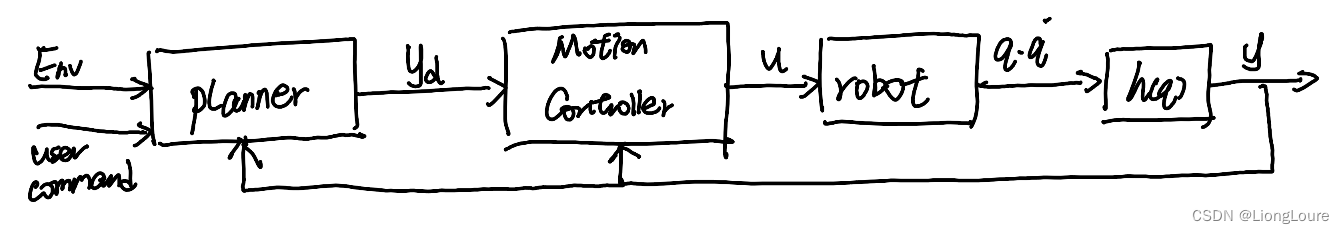
often times q d q_{\mathrm{d}} qd is given by planner represented by polynomials , so that q ˙ d , q ¨ d \dot{q}_{\mathrm{d}},\ddot{q}_{\mathrm{d}} q˙d,q¨d can be easily obtained
2.2 Variations in Robot Motion Control
-
Joint-space vs. Task-space control
Joint-space : y ( t ) = q ( t ) y\left( t \right) =q\left( t \right) y(t)=q(t) , i.e. , want q ( t ) q\left( t \right) q(t) to track a given q d ( t ) q_{\mathrm{d}}\left( t \right) qd(t) joint reference
Task-space : y ( t ) = [ T ( q ( t ) ) ] ∈ S E ( 3 ) y\left( t \right) =\left[ T\left( q\left( t \right) \right) \right] \in SE\left( 3 \right) y(t)=[T(q(t))]∈SE(3) denotes end-effector pose/configuration, we want y ( t ) y\left( t \right) y(t) to track y d ( t ) y_{\mathrm{d}}\left( t \right) yd(t) -
Actuation models:
Velocity source : u = q ˙ u=\dot{q} u=q˙ —— directly control velocity
Acceleration sources : u = q ¨ u=\ddot{q} u=q¨ —— directly control acceleration
Torque sources : u = τ u=\tau u=τ —— directly control torque

Acutation model make sense if for ant given u u u , the joint velocity q ˙ \dot{q} q˙ can immediatly reach u u u
Motion Control Problem
Design u u u to set y y y track desired reference y d y_{\mathrm{d}} yd
- Depending on our assumption on u / y u/y u/y
output y y y —— 6大基本问题
y ↔ q ∈ R n y\leftrightarrow q\in \mathbb{R} ^n y↔q∈Rn - joint variable : Joint space motion control (Velocity-resolved Joint-space control ; Acceleration-resolved Joint-space control ; Torque-resolved Joint-space control ; )
y ↔ [ T ( q ) ] ∈ S E ( 3 ) y\leftrightarrow \left[ T\left( q \right) \right] \in SE\left( 3 \right) y↔[T(q)]∈SE(3) or y = f ( q ) y=f\left( q \right) y=f(q) - task space variable - e.g. origin of end-effector frame : Task space motion control (Velocity-resolved Task-space ; Acceleration-resolved Task-space ; Torque-resolved Task-space ; )
Linear control / feedback lineariazation
3. Motion Control with Velocity/Acceleration as Input
3.1 Velocity-Resolved Control
Each joints’ velocity q ˙ i \dot{q}_{\mathrm{i}} q˙i can be directly controlled
Good approximation for hydraulic actuators
Common approxiamtion of the outer-loop control for the Inner / outer loop control setup

3.2.1 Velocity-Resolved Joint Space Control
Joint-space ‘dynamics’ : single integrator q ˙ = u \dot{q}=u q˙=u
Joint-space tracking becomes standard linear tracking control problem : u = q ˙ d + K 0 q ¨ ⇒ q ~ ˙ + K 0 q ¨ = 0 u=\dot{q}_{\mathrm{d}}+K_0\ddot{q}\Rightarrow \dot{\tilde{q}}+K_0\ddot{q}=0 u=q˙d+K0q¨⇒q~˙+K0q¨=0 , where q ~ = q d − q \tilde{q}=q_{\mathrm{d}}-q q~=qd−q is the joint position error. —— stable if e i g ( − K 0 ) ∈ O L H P eig\left( -K_0 \right) \in OLHP eig(−K0)∈OLHP
The error dynamic is stable if − K 0 -K_0 −K0 is Hurwitz
3.2.2 Velocity-Resolved Task Space Control
For task space control , y = [ T ( q ) ] y=\left[ T\left( q \right) \right] y=[T(q)] needs to track y d y_{\mathrm{d}} yd , y y y can be ant function of q q q, in particular , it can represents position and/or the end-effector frame
Taking derivatives of y y y , and letting u = q ˙ u=\dot{q} u=q˙ , we have : y ˙ = J a ( q ) u \dot{y}=J_{\mathrm{a}}\left( q \right) u y˙=Ja(q)u
Note that q q q is function of y y y through inverse kinematics ( q = I K ( y ) q=IK\left( y \right) q=IK(y))
So the above dynamics can be written in terms of y y y and u u u only. The detailed form can be quite complex in general y ˙ = J a ( I K ( y ) ) u \dot{y}=J_{\mathrm{a}}\left( IK\left( y \right) \right) u y˙=Ja(IK(y))u
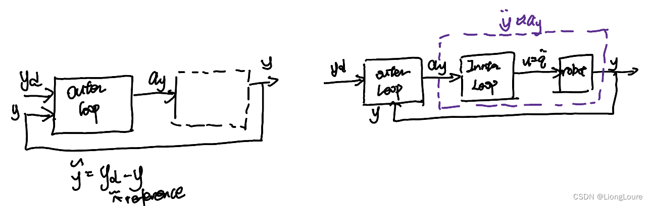
- Let v y v_{\mathrm{y}} vy be virtual control y ˙ = v y \dot{y}=v_{\mathrm{y}} y˙=vy design v y v_{\mathrm{y}} vy to track y d y_{\mathrm{d}} yd (same as above)
- Find actual control u u u such that J a ( I K ( y ) ) u ≈ v y J_{\mathrm{a}}\left( IK\left( y \right) \right) u\approx v_{\mathrm{y}} Ja(IK(y))u≈vy


We can design outer-loop controller as if we can directly control y ˙ \dot{y} y˙
y ˙ = v y = y ˙ d + K ( y d − y ) ⟹ p l u g i n y ˙ = v y y ~ ˙ = − K y ~ \dot{y}=v_{\mathrm{y}}=\dot{y}_{\mathrm{d}}+K\left( y_{\mathrm{d}}-y \right) \overset{plug\,\,in\,\,\dot{y}=v_{\mathrm{y}}\,\,}{\Longrightarrow}\dot{\tilde{y}}=-K\tilde{y} y˙=vy=y˙d+K(yd−y)⟹pluginy˙=vyy~˙=−Ky~
We can select K K K such that − K -K −K is Hurtwiz , object of inner loop : determine u = q ˙ u=\dot{q} u=q˙ such that y ˙ ≈ v y \dot{y}\approx v_{\mathrm{y}} y˙≈vy
System(2) is nonlinear system , a commeon way is to break it into inner-outer loop , where the outer loop directly control velocity of y y y, and the inner loop tries to find u u u to generate desired task space velocity
Outer loop : y ˙ = v y \dot{y}=v_{\mathrm{y}} y˙=vy , where control v y = y ˙ d + K 0 y ~ v_{\mathrm{y}}=\dot{y}_{\mathrm{d}}+K_0\tilde{y} vy=y˙d+K0y~ , resulting in task-space closed-loop error dynamics: y ~ ˙ + K 0 y ~ = 0 \dot{\tilde{y}}+K_0\tilde{y}=0 y~˙+K0y~=0
Above task space tracking relies on a fictitious control v y v_{\mathrm{y}} vy , i.e. , it assumes y ˙ \dot{y} y˙ can be arbitrarily controlled by selecting appropriate u = q ˙ u=\dot{q} u=q˙ , which is true if J a J_{\mathrm{a}} Ja is full-row rank
Inner loop : Given v y v_{\mathrm{y}} vy from the outer loop, find the joint velocity control by solving
{ min u ∥ v y − J a ( q ) u ∥ 2 + r e g u l a r i z a t i o n t e r m s u b j . t o : C o n s t r a i n t s o n u , e . g . { q ˙ min ⩽ u ⩽ q ˙ max q min ⩽ q + u Δ t ⩽ q max \begin{cases} \min _{\mathrm{u}}\left\| v_{\mathrm{y}}-J_{\mathrm{a}}\left( q \right) u \right\| ^2+regularization\,\,term\\ subj.to\,\,: Constraints\,\,on\,\,u\,\,, e.g.\begin{cases} \dot{q}_{\min}\leqslant u\leqslant \dot{q}_{\max}\\ q_{\min}\leqslant q+u\varDelta t\leqslant q_{\max}\\ \end{cases}\\ \end{cases} ⎩ ⎨ ⎧minu∥vy−Ja(q)u∥2+regularizationtermsubj.to:Constraintsonu,e.g.{q˙min⩽u⩽q˙maxqmin⩽q+uΔt⩽qmax
Inner-loop is essentially a differential IK controller
One can also use the pseudo-inverse control u = J a † v y u={J_{\mathrm{a}}}^{\dagger}v_{\mathrm{y}} u=Ja†vy
3.2 Acceleration-Resolved Control
3.2.1 Acceleration-Resolved Control in Joint Space
Joint acceleration cna be directly controlled , resulting in double-integrator dynamics q ¨ = u \ddot{q}=u q¨=u . Given q d q_{\mathrm{d}} qd reference , we want q → q d q\rightarrow q_{\mathrm{d}} q→qd (double integartor)
Joint-space tracking becomes standard linear tracking control problem for double-integrator system:
u = q ¨ d + K 1 q ~ ˙ + K 0 q ~ = 0 , q ~ ∈ R n u=\ddot{q}_{\mathrm{d}}+K_1\dot{\tilde{q}}+K_0\tilde{q}=0,\tilde{q}\in \mathbb{R} ^n u=q¨d+K1q~˙+K0q~=0,q~∈Rn
—— PD control , closed-loop system , where q ~ = q d − q \tilde{q}=q_{\mathrm{d}}-q q~=qd−q is the joint position error.
Stablility condition : Let x = [ q ~ q ~ ˙ ] ∈ R 2 n x=\left[ \begin{array}{c} \tilde{q}\\ \dot{\tilde{q}}\\ \end{array} \right] \in \mathbb{R} ^{2n} x=[q~q~˙]∈R2n , [ 0 E − K 0 − K 1 ] [ q ~ q ~ ˙ ] , x ˙ = A x \left[ \begin{matrix} 0& E\\ -K_0& -K_1\\ \end{matrix} \right] \left[ \begin{array}{c} \tilde{q}\\ \dot{\tilde{q}}\\ \end{array} \right] ,\dot{x}=Ax [0−K0E−K1][q~q~˙],x˙=Ax
closed-loop system is stable . if e i g ( A ) ∈ O L H P eig\left( A \right) \in OLHP eig(A)∈OLHP or A A A is Hurwitz
3.2.2 Acceleration-Resolved Control in Task Space
For task space control , y = [ T ( q ) ] ∈ S E ( 3 ) y=\left[ T\left( q \right) \right] \in SE\left( 3 \right) y=[T(q)]∈SE(3) needs to track y d y_{\mathrm{d}} yd

Note : For y = f ( q ) y=f\left( q \right) y=f(q) y ˙ = J a ( q ) q ˙ \dot{y}=J_{\mathrm{a}}\left( q \right) \dot{q} y˙=Ja(q)q˙ and y ¨ = J ˙ a ( q ) q ˙ + J a ( q ) q ¨ ⇒ y ¨ = J ˙ a ( q ) q ˙ + J a ( q ) u ⇐ \ddot{y}=\dot{J}_{\mathrm{a}}\left( q \right) \dot{q}+J_{\mathrm{a}}\left( q \right) \ddot{q}\Rightarrow \ddot{y}=\dot{J}_{\mathrm{a}}\left( q \right) \dot{q}+J_{\mathrm{a}}\left( q \right) u\Leftarrow y¨=J˙a(q)q˙+Ja(q)q¨⇒y¨=J˙a(q)q˙+Ja(q)u⇐ nonlinear dynamics
Following the same inner-outer loop strategy deiscussed before . Introduce virtual control , a y a_{\mathrm{y}} ay such that y ¨ = a y \ddot{y}=a_{\mathrm{y}} y¨=ay , we can design controller for a y a_{\mathrm{y}} ay to let y → y d y\rightarrow y_{\mathrm{d}} y→yd
Outer-loop dynamics : y ¨ = a y \ddot{y}=a_{\mathrm{y}} y¨=ay , with a y a_{\mathrm{y}} ay being the outer-loop control input a y = y ¨ d + K 1 y ~ ˙ + K 0 y ~ ⇒ y ~ ¨ + K 1 y ~ ˙ + K 0 y ~ = 0 a_{\mathrm{y}}=\ddot{y}_{\mathrm{d}}+K_1\dot{\tilde{y}}+K_0\tilde{y}\Rightarrow \ddot{\tilde{y}}+K_1\dot{\tilde{y}}+K_0\tilde{y}=0 ay=y¨d+K1y~˙+K0y~⇒y~¨+K1y~˙+K0y~=0
—— PD control , stable if [ 0 E − K 0 − K 1 ] \left[ \begin{matrix} 0& E\\ -K_0& -K_1\\ \end{matrix} \right] [0−K0E−K1] Hurwitz
Inner-loop : given a y a_{\mathrm{y}} ay from outer loop , find the “best” joint acceleration:
{ min u ∥ a y − J ˙ a ( q ) q ˙ − J a ( q ) u ∥ 2 + r e g u l a r i z a t i o n t e r m s u b j . t o : C o n s t r a i n t s o n u \begin{cases} \min _{\mathrm{u}}\left\| a_{\mathrm{y}}-\dot{J}_{\mathrm{a}}\left( q \right) \dot{q}-J_{\mathrm{a}}\left( q \right) u \right\| ^2+regularization\,\,term\\ subj.to\,\,: Constraints\,\,on\,\,u\,\,\\ \end{cases} ⎩ ⎨ ⎧minu ay−J˙a(q)q˙−Ja(q)u 2+regularizationtermsubj.to:Constraintsonu
—— u u u : optimization variable , J ˙ a ( q ) , q ˙ , q \dot{J}_{\mathrm{a}}\left( q \right) ,\dot{q},q J˙a(q),q˙,q - known
{ A c c : q ¨ min ⩽ u ⩽ q ¨ max V e l : q ˙ min ⩽ q + u Δ t ⩽ q ˙ max \begin{cases} Acc\,\,: \ddot{q}_{\min}\leqslant u\leqslant \ddot{q}_{\max}\\ Vel\,\,: \dot{q}_{\min}\leqslant q+u\varDelta t\leqslant \dot{q}_{\max}\\ \end{cases} {Acc:q¨min⩽u⩽q¨maxVel:q˙min⩽q+uΔt⩽q˙max
Mathematically , the above problem is the same as the Differential IK problem
At any given time , q ˙ , q \dot{q},q q˙,q can be measured , and then y , y ˙ y,\dot{y} y,y˙ can be computed, which allows us to compute outer loop control a y a_{\mathrm{y}} ay and inner loop control u u u
4. Motion Control with Torque as Input and Task Space Inverse Dynamics
4.1 Recall Properties of Robot Dynamics
For fully actuated robot :
τ = M ( q ) q ¨ + C ( q , q ˙ ) q ˙ + g ( q ) \tau =M\left( q \right) \ddot{q}+C\left( q,\dot{q} \right) \dot{q}+g\left( q \right) τ=M(q)q¨+C(q,q˙)q˙+g(q)
M ( q ) = ∑ J i T [ I i ] 6 × 6 J i ∈ R n × n M\left( q \right) =\sum{{J_{\mathrm{i}}}^{\mathrm{T}}\left[ \mathcal{I} _{\mathrm{i}} \right] _{6\times 6}J_{\mathrm{i}}}\in \mathbb{R} ^{n\times n} M(q)=∑JiT[Ii]6×6Ji∈Rn×n
There are many valid difinitions of C ( q , q ˙ ) C\left( q,\dot{q} \right) C(q,q˙) , typical choice for C C C include:
C i j = ∑ k 1 2 ( ∂ M i j ∂ q k + ∂ M i k ∂ q j − ∂ M j k ∂ q i ) C_{\mathrm{ij}}=\sum_k^{}{\frac{1}{2}\left( \frac{\partial M_{\mathrm{ij}}}{\partial q_{\mathrm{k}}}+\frac{\partial M_{\mathrm{ik}}}{\partial q_{\mathrm{j}}}-\frac{\partial M_{\mathrm{jk}}}{\partial q_{\mathrm{i}}} \right)} Cij=∑k21(∂qk∂Mij+∂qj∂Mik−∂qi∂Mjk)
For the above defined C C C , we have M ˙ − 2 C \dot{M}-2C M˙−2C is skew symmetric
For all valid C C C, we have q ˙ T [ M ˙ − 2 C ] q ˙ = 0 \dot{q}^{\mathrm{T}}\left[ \dot{M}-2C \right] \dot{q}=0 q˙T[M˙−2C]q˙=0
These properties play improtant role in designing motion controller
4.2 Computed Torque Control
For fully-actuated robot, we have M ( q ) ≻ 0 M\left( q \right) \succ 0 M(q)≻0 and q ¨ \ddot{q} q¨ can be arbitrarily specified through torque control u = τ u=\tau u=τ
q ¨ = M − 1 ( q ) [ u − C ( q , q ˙ ) q ˙ − g ( q ) ] \ddot{q}=M^{-1}\left( q \right) \left[ u-C\left( q,\dot{q} \right) \dot{q}-g\left( q \right) \right] q¨=M−1(q)[u−C(q,q˙)q˙−g(q)]
we know how to design controller if u = q ¨ u=\ddot{q} u=q¨

Thus , for fully-acuated robot, torque controlled case can be reduced to the acceleration-resolved case
Outer loop: q ¨ = a q \ddot{q}=a_{\mathrm{q}} q¨=aq with joint acceleration as control input
a q = q ¨ + K 1 y ~ ˙ + K 0 y ~ ⇒ q ~ ¨ + K 1 q ~ ˙ + K 0 q ~ = 0 a_{\mathrm{q}}=\ddot{q}+K_1\dot{\tilde{y}}+K_0\tilde{y}\Rightarrow \ddot{\tilde{q}}+K_1\dot{\tilde{q}}+K_0\tilde{q}=0 aq=q¨+K1y~˙+K0y~⇒q~¨+K1q~˙+K0q~=0
Inner loop : since M ( q ) M\left( q \right) M(q) is square and nonsingular , inner loop control u u u can be found analytically:
u = M ( q ) ( q ¨ d + K 1 q ~ ˙ + K 0 q ~ ) + C ( q , q ˙ ) q ˙ + g ( q ) u=M\left( q \right) \left( \ddot{q}_{\mathrm{d}}+K_1\dot{\tilde{q}}+K_0\tilde{q} \right) +C\left( q,\dot{q} \right) \dot{q}+g\left( q \right) u=M(q)(q¨d+K1q~˙+K0q~)+C(q,q˙)q˙+g(q)

The control law is a function of q , q ˙ q,\dot{q} q,q˙ and the reference q d q_{\mathrm{d}} qd. It is called computed-torque control.
The control law also relies on system model M , C , g M,C,g M,C,g if these model information are not accurate, the control will not perform well.
y = f ( q ) , y ¨ = J ˙ a ( q ) q ˙ + J a ( q ) M − 1 ( u − C − g ) y=f\left( q \right) ,\ddot{y}=\dot{J}_{\mathrm{a}}\left( q \right) \dot{q}+J_{\mathrm{a}}\left( q \right) M^{-1}\left( u-C-g \right) y=f(q),y¨=J˙a(q)q˙+Ja(q)M−1(u−C−g)
Idea easily extends to task space : y ˙ = J a ( q ) q ˙ \dot{y}=J_{\mathrm{a}}\left( q \right) \dot{q} y˙=Ja(q)q˙ and y ¨ = J ˙ a ( q ) q ˙ + J a ( q ) q ¨ \ddot{y}=\dot{J}_{\mathrm{a}}\left( q \right) \dot{q}+J_{\mathrm{a}}\left( q \right) \ddot{q} y¨=J˙a(q)q˙+Ja(q)q¨ —— τ = u = τ , q ¨ = M − 1 [ u − C − g ] \tau =u=\tau ,\ddot{q}=M^{-1}\left[ u-C-g \right] τ=u=τ,q¨=M−1[u−C−g]
Outer loop : y ¨ = a y \ddot{y}=a_{\mathrm{y}} y¨=ay and a y = y ¨ d + K 1 y ~ ˙ + K 0 y ~ a_{\mathrm{y}}=\ddot{y}_{\mathrm{d}}+K_1\dot{\tilde{y}}+K_0\tilde{y} ay=y¨d+K1y~˙+K0y~
Inner loop : sekect torque control u = τ u=\tau u=τ by
{ min u ∥ a y − J ˙ a ( q ) q ˙ − J a ( q ) M − 1 ( u − C q ˙ − g ) ∥ 2 s u b j . t o : C o n s t r a i n t s \begin{cases} \min _{\mathrm{u}}\left\| a_{\mathrm{y}}-\dot{J}_{\mathrm{a}}\left( q \right) \dot{q}-J_{\mathrm{a}}\left( q \right) M^{-1}\left( u-C\dot{q}-g \right) \right\| ^2\\ subj.to\,\,: Constraints\,\,\\ \end{cases} ⎩ ⎨ ⎧minu ay−J˙a(q)q˙−Ja(q)M−1(u−Cq˙−g) 2subj.to:Constraints
If J a J_{\mathrm{a}} Jais invertible and we don’t impose additional torque constraints, analytical control law can be easily obtained —— u = ( J a ( q ) M − 1 ) − 1 ( a y − J ˙ a ( q ) q ˙ . . . ) u=\left( J_{\mathrm{a}}\left( q \right) M^{-1} \right) ^{-1}\left( a_{\mathrm{y}}-\dot{J}_{\mathrm{a}}\left( q \right) \dot{q}... \right) u=(Ja(q)M−1)−1(ay−J˙a(q)q˙...)
4.3 Inverse Dynamics Control
The computed-torque controller above is also canned inverse dynamics control
Forward dynamics : given τ \tau τ to compute q ¨ \ddot{q} q¨ —— from torque to motion
Inverse dynamics : given desired acceleration a q a_{\mathrm{q}} aq, we inverted it to find the required control by u = M a q + C q ˙ + g u=Ma_{\mathrm{q}}+C\dot{q}+g u=Maq+Cq˙+g
Task space case can be viewed as inverting the task space dynamics —— Given a y a_{\mathrm{y}} ay ( y y y task space) , find τ \tau τ such that y ¨ = a y \ddot{y}=a_{\mathrm{y}} y¨=ay
With recent advances in optimization , it is often preferred to do ID with quedratic program
For example, above equation can be viewed as task-space ID. We can incorporate torque contraints explicitly as follows:
{ min u ∥ a y − J ˙ a ( q ) q ˙ − J a M − 1 ( u − C q ˙ − g ) ∥ 2 s u b j . t o : u − ⩽ u ⩽ u + \begin{cases} \min _{\mathrm{u}}\left\| a_{\mathrm{y}}-\dot{J}_{\mathrm{a}}\left( q \right) \dot{q}-J_{\mathrm{a}}M^{-1}\left( u-C\dot{q}-g \right) \right\| ^2\\ subj.to\,\,: u_-\leqslant u\,\,\leqslant u_+\,\,\\ \end{cases} ⎩ ⎨ ⎧minu ay−J˙a(q)q˙−JaM−1(u−Cq˙−g) 2subj.to:u−⩽u⩽u+
optimization variable u ∈ R n u\in \mathbb{R} ^n u∈Rn
This is equivalent to the following more popular form:
{ min u , q ¨ ∥ a y − J ˙ a q ˙ − J a q ¨ ∥ 2 s u b j . t o : M q ¨ + C q ˙ + g = u u − ⩽ u ∈ R n ⩽ u + \begin{cases} \underset{u,\ddot{q}}{\min}\left\| a_{\mathrm{y}}-\dot{J}_{\mathrm{a}}\dot{q}-J_{\mathrm{a}}\ddot{q} \right\| ^2\\ subj.to\,\,: \begin{array}{c} M\ddot{q}+C\dot{q}+g=u\\ u_-\leqslant u\in \mathbb{R} ^n\,\,\leqslant u_+\,\,\\ \end{array}\\ \end{cases} ⎩ ⎨ ⎧u,q¨min ay−J˙aq˙−Jaq¨ 2subj.to:Mq¨+Cq˙+g=uu−⩽u∈Rn⩽u+
optimization variable u , q ¨ ∈ R n u,\ddot{q}\in \mathbb{R} ^n u,q¨∈Rn
相关文章:
[足式机器人]Part4 南科大高等机器人控制课 CH12 Robotic Motion Control
本文仅供学习使用 本文参考: B站:CLEAR_LAB 笔者带更新-运动学 课程主讲教师: Prof. Wei Zhang 课程链接 : https://www.wzhanglab.site/teaching/mee-5114-advanced-control-for-robotics/ 南科大高等机器人控制课 Ch12 Robotic …...
)
【C++】知识点汇总(上)
C知识点复习上 一、C 概述1. 基本数据类型2. 变量定义和访问3. 常量与约束访问 二、程序控制结构详解与示例1. 表达式2. 选择控制2.1 if 语句2.2 switch 语句 3. 循环控制3.1 for 循环3.2 while 循环3.3 do-while 循环 4. goto 语句5. 控制语句的嵌套 三、函数1. 函数的定义和调…...

解决docker容器内无法连接宿主redis
背景 小程序的发短信服务挂了,随查看日志,该报错日志如下 Error 111 connecting to 127.0.0.1:6379. Connection refused. 6379是监听redis服务的端口,那大概是redis出错了。 首先查看了redis是否正常启动,检查出服务正常。 由于小…...
43 tmpfs/devtmpfs 文件系统
前言 在 linux 中常见的文件系统 有很多, 如下 基于磁盘的文件系统, ext2, ext3, ext4, xfs, btrfs, jfs, ntfs 内存文件系统, procfs, sysfs, tmpfs, squashfs, debugfs 闪存文件系统, ubifs, jffs2, yaffs 文件系统这一套体系在 linux 有一层 vfs 抽象, 用户程序不用…...
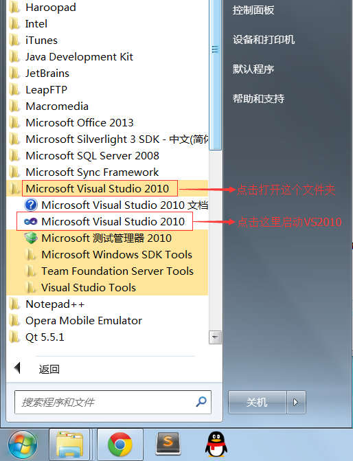
C语言编译器(C语言编程软件)完全攻略(第十二部分:VS2010下载地址和安装教程(图解))
介绍常用C语言编译器的安装、配置和使用。 十二、VS2010下载地址和安装教程(图解) 为了更好地支持 Win7 程序的开发,微软于2010年4月12日发布了 VS2010,它的界面被重新设计,变得更加简洁。需要注意的是,V…...

【VRTK】【VR开发】【Unity】18-VRTK与Unity UI控制的融合使用
课程配套学习项目源码资源下载 https://download.csdn.net/download/weixin_41697242/88485426?spm=1001.2014.3001.5503 【背景】 VRTK和Unity自身的UI控制包可以配合使用发挥效果。本篇就讨论这方面的实战内容。 之前可以互动的立体UI并不是传统的2D UI对象,在实际使用中…...
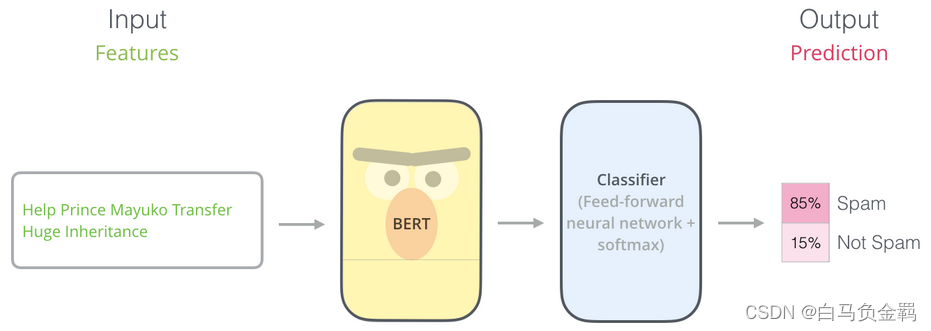
BERT(从理论到实践): Bidirectional Encoder Representations from Transformers【3】
这是本系列文章中的第3弹,请确保你已经读过并了解之前文章所讲的内容,因为对于已经解释过的概念或API,本文不会再赘述。 本文要利用BERT实现一个“垃圾邮件分类”的任务,这也是NLP中一个很常见的任务:Text Classification。我们的实验环境仍然是Python3+Tensorflow/Keras…...

静态网页设计——校园官网(HTML+CSS+JavaScript)
前言 声明:该文章只是做技术分享,若侵权请联系我删除。!! 使用技术:HTMLCSSJS 主要内容:对学校官网的结构进行模仿,对布局进行模仿。 主要内容 1、首页 首页以多个div对页面进行分割和布局…...
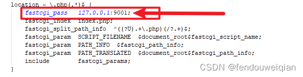
phpstudy_pro 关于多版本php的问题
我在phpstudy中安装了多个PHP版本 我希望不同的网站可以对应不同的PHP版本,则在nginx配置文件中需要知道不同的PHP版本的监听端口是多少,如下图所示 然而找遍了php.ini配置,并未对listen进行设置,好奇是怎么实现不同的PHP监听不同…...
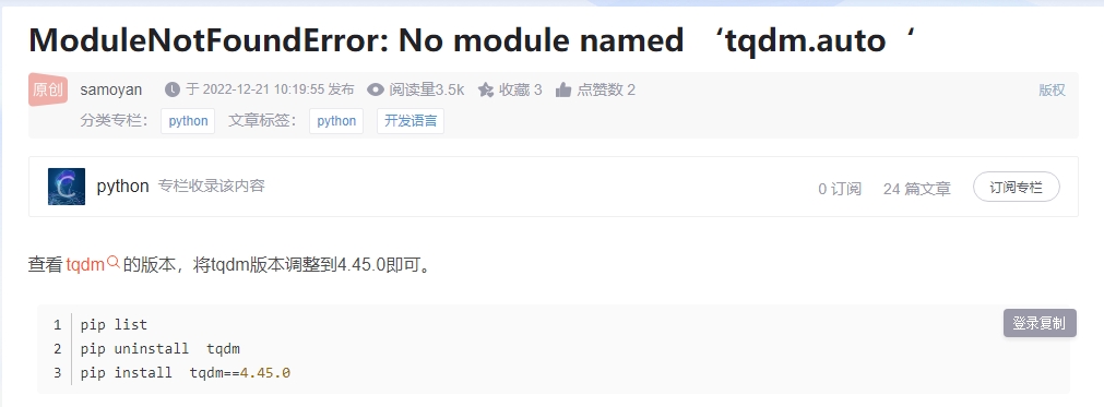
TemporalKit的纯手动安装
最近在用本地SD安装temporalkit插件 本地安装插件最常见的问题就是,GitCommandError:… 原因就是,没有科学上网,而且即使搭了ladder,在SD的“从网址上安装”或是“插件安装”都不行,都不行!!&am…...
人生重开模拟器
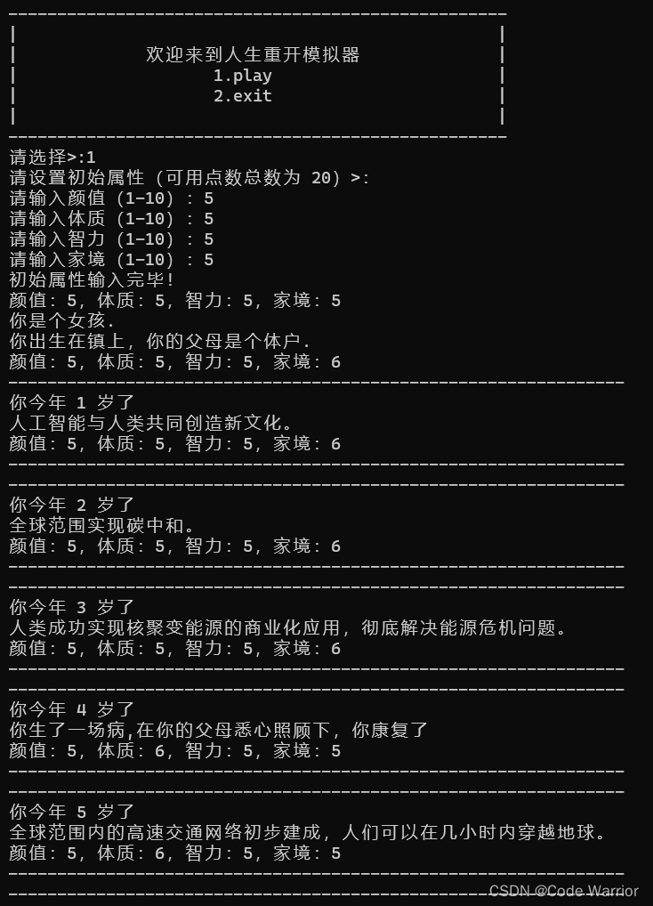
前言: 人生重开模拟器是前段时间非常火的一个小游戏,接下来我们将一起学习使用c语言写一个简易版的人生重开模拟器。 网页版游戏: 人生重开模拟器 (ytecn.com) 1.实现一个简化版的人生重开模拟器 (1) 游戏开始的时…...

优化算法3D可视化
编程实现优化算法,并3D可视化 1. 函数3D可视化 分别画出 和 的3D图 import numpy as np from matplotlib import pyplot as plt import torch# 画出x**2 class Op(object):def __init__(self):passdef __call__(self, inputs):return self.forward(inputs)def for…...
魔术表演Scratch-第14届蓝桥杯Scratch省赛真题第1题
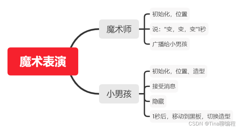
1.魔术表演(20分) 评判标准: 4分:满足"具体要求"中的1); 8分:满足"具体要求"中的2); 8分,满足"具体要求"中的3)…...
LLM 中的长文本问题
近期,随着大模型技术的发展,长文本问题逐渐成为热门且关键的问题,不妨简单梳理一下近期出现的典型的长文本模型: 10 月上旬,Moonshot AI 的 Kimi Chat 问世,这是首个支持 20 万汉字输入的智能助手产品; 10 月下旬,百川智能发布 Baichuan2-192K 长窗口大模型,相当于一次…...

深入了解Swagger注解:@ApiModel和@ApiModelProperty实用指南
在现代软件开发中,提供清晰全面的 API 文档 至关重要。ApiModel 和 ApiModelProperty 这样的代码注解在此方面表现出色,通过增强模型及其属性的元数据来丰富文档内容。它们的主要功能是为这些元素命名和描述,使生成的 API 文档更加明确。 Api…...
Linux学习第48天:Linux USB驱动试验:保持热情,保持节奏,持续学习是作为一个技术人员应有的基本素质和要求
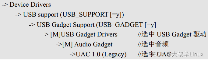
Linux版本号4.1.15 芯片I.MX6ULL 大叔学Linux 品人间百味 思文短情长 最近更新的速度和频率大不如以前,主要原因还是自己有些懈怠了。学习是一个持续努力的过程,一旦中断,再想保持以往的状态可能要…...

数据库索引简析
文章目录 前言一、索引是什么二、索引的有什么用三、索引的分类四、索引的数据结构总结 前言 在我们使用数据库的过程中,往往会碰到一个叫做索引的东西,不管是表的设计,还是数据库性能的优化往往都会涉及到索引。那么他是个什么东西ÿ…...
leetcode贪心(单调递增的数字、监控二叉树)
738.单调递增的数字 给定一个非负整数 N,找出小于或等于 N 的最大的整数,同时这个整数需要满足其各个位数上的数字是单调递增。 (当且仅当每个相邻位数上的数字 x 和 y 满足 x < y 时,我们称这个整数是单调递增的。ÿ…...

如何在win7同样支持Webview2 在 WPF 中使用本地 Webview2 ,如何不依赖系统 Runtime
项目运行环境: .Net Framework 4.5.2 Windows 7 x64 Service Pack 1 WebView2 Microsoft.WebView2.FixedVersionRuntime.120.0.2210.91.x64 考虑到很多老项目,本项目使用的是.Net Framework 4.5.2,.Net 更高版本的其实也是可以支持的。 …...

【docker】网络模式管理
目录 一、Docker网络实现原理 二、Docker的网络模式 1、host模式 1.1 host模式原理 1.2 host模式实操 2、Container模式 2.2 container模式实操 3、none模式 4、bridger模式 4.1 bridge模式的原理 4.2 bridge实操 5、overlay模式 6、自定义网络模式 6.1 为什么需要…...
实战复盘:从外网突破到域控的完整攻击链剖析)
红日靶场(vulnstack)实战复盘:从外网突破到域控的完整攻击链剖析
1. 红日靶场环境搭建与拓扑解析 红日靶场(vulnstack)是国内知名的渗透测试实战平台,模拟了真实企业网络环境中常见的漏洞场景。这个靶场特别适合想要系统学习内网渗透技术的新手,我自己第一次接触时就被它贴近实战的设计惊艳到了。…...

如何在5分钟内用Blender创建专业级分子可视化效果
如何在5分钟内用Blender创建专业级分子可视化效果 【免费下载链接】blender-chemicals Draws chemicals in Blender using common input formats (smiles, molfiles, cif files, etc.) 项目地址: https://gitcode.com/gh_mirrors/bl/blender-chemicals 还在为制作分子结…...

So-Bridge:轻量级跨语言进程通信库的设计与实践
1. 项目概述:一个连接不同世界的“桥梁” 最近在折腾一些自动化脚本和数据处理流程时,我遇到了一个挺典型的问题:手头的工具和系统五花八门,有的用Python写,有的依赖Node.js环境,还有的干脆是独立的可执行文…...

ESP32接入ChatGPT API:打造智能语音交互硬件原型
1. 项目概述:当ESP32遇见ChatGPT最近在捣鼓ESP32,想给它加点“脑子”。ESP32本身是个很棒的物联网微控制器,Wi-Fi、蓝牙、低功耗,该有的都有,但它本质上还是个执行预设逻辑的设备。我就琢磨,能不能让它接入…...

对比官方价,Taotoken活动价带来的Token成本优势感知
🚀 告别海外账号与网络限制!稳定直连全球优质大模型,限时半价接入中。 👉 点击领取海量免费额度 对比官方价,Taotoken活动价带来的Token成本优势感知 1. 引言:从固定成本到按需消耗 对于个人开发者或小型…...
)
Qt实战:用QAbstractTableModel和QTableView打造一个带复选框和下拉框的工业数据表格(附完整源码)
Qt工业级数据表格开发实战:基于模型/视图架构的高级交互实现 在工业自动化软件领域,数据表格作为人机交互的核心组件,承担着参数配置、状态监控和工艺管理等多重职责。传统QTableWidget虽然简单易用,但在处理SMT贴片机这类需要管理…...

Aider:AI结对编程实战,从原理到项目级代码编辑
1. 项目概述:当AI成为你的结对编程伙伴如果你是一名开发者,大概率经历过这样的场景:面对一个需要修改的复杂函数,你清楚地知道要做什么,但就是不想动手去敲那一行行重复或繁琐的代码;或者,在深夜…...

Python实战:利用pymodbus构建工业数据采集与监控系统
1. 工业数据采集为什么需要Modbus? 在工厂车间里,你可能见过各种钢铁巨兽般的设备——数控机床、PLC控制器、温度传感器。这些设备每天都在产生海量数据,但如何让这些"哑巴设备"开口说话?Modbus协议就是它们的通用语言。…...

Excel数据分析工具库 vs. Python手动计算:手把手教你搞定一元线性回归的全部检验
Excel与Python双视角解析:一元线性回归的实战检验指南 当市场部的同事递给你一份用户行为数据,指着"页面停留时间"和"转化率"两列问你"这两个指标到底有没有关系"时,你会选择打开Excel的回归分析工具一键生成报…...

4 个新的流行 AI 概念及其在数字产品中的潜力
原文:towardsdatascience.com/the-4-new-trendy-ai-concepts-and-their-potential-in-digital-products-cf5e1b85bff9 https://github.com/OpenDocCN/towardsdatascience-blog-zh-2024/raw/master/docs/img/79c8534a324cff796ff9200cb0207d8a.png 图片由Joshua Col…...