C2_W2_Assignment_吴恩达_中英_Pytorch
Neural Networks for Handwritten Digit Recognition, Multiclass
In this exercise, you will use a neural network to recognize the hand-written digits 0-9.
在本次练习中,您将使用神经网络来识别0-9的手写数字。
Outline
- 1 - Packages
- 2 - ReLU Activation
- 3 - Softmax Function
- Exercise 1
- 4 - Neural Networks
- 4.1 Problem Statement
- 4.2 Dataset
- 4.3 Model representation
- 4.4 Tensorflow Model Implementation
- 4.5 Softmax placement
- Exercise 2
1 - Packages
First, let’s run the cell below to import all the packages that you will need during this assignment.
首先,运行下面的单元格来导入你在这个练习中需要的所有包。
- numpy is the fundamental package for scientific computing with Python.
- matplotlib is a popular library to plot graphs in Python.
- tensorflow a popular platform for machine learning.
import numpy as np
import tensorflow as tf
from tensorflow.keras.models import Sequential
from tensorflow.keras.layers import Dense
from tensorflow.keras.activations import linear, relu, sigmoid
%matplotlib widget
import matplotlib.pyplot as plt
plt.style.use('./deeplearning.mplstyle')import logging
logging.getLogger("tensorflow").setLevel(logging.ERROR)
tf.autograph.set_verbosity(0)from public_tests import * from autils import *
from lab_utils_softmax import plt_softmax
np.set_printoptions(precision=2)
2 - ReLU Activation
This week, a new activation was introduced, the Rectified Linear Unit (ReLU).
本周,一个新的激活函数被引入,即整流线性单元(ReLU)。
a = m a x ( 0 , z ) ReLU function a = max(0,z) \quad\quad\text {ReLU function} a=max(0,z)ReLU function
plt_act_trio()


The example from the lecture on the right shows an application of the ReLU. In this example, the derived “awareness” feature is not binary but has a continuous range of values. The sigmoid is best for on/off or binary situations. The ReLU provides a continuous linear relationship. Additionally it has an ‘off’ range where the output is zero.
右边的例子展示了ReLU的一个应用。在这个例子中,派生的“意识”特征不是二元的,而是具有连续范围的值。s型最适合开/关或二进制的情况。ReLU提供了一个连续的线性关系。此外,它有一个输出为零的“关闭”范围
The “off” feature makes the ReLU a Non-Linear activation. Why is this needed? This enables multiple units to contribute to to the resulting function without interfering. This is examined more in the supporting optional lab.
“关闭”功能使ReLU成为非线性激活。为什么需要这样做?这使得多个单元能够在不干扰的情况下为最终功能做出贡献。在配套的可选实验室中对此进行了更多的研究
3 - Softmax Function
A multiclass neural network generates N outputs. One output is selected as the predicted answer. In the output layer, a vector z \mathbf{z} z is generated by a linear function which is fed into a softmax function. The softmax function converts z \mathbf{z} z into a probability distribution as described below. After applying softmax, each output will be between 0 and 1 and the outputs will sum to 1. They can be interpreted as probabilities. The larger inputs to the softmax will correspond to larger output probabilities.
一个多类神经网络产生N个输出。选择一个输出作为预测答案。在输出层,向量 z \mathbf{z} z是由一个线性函数生成的,该线性函数被馈送到一个softmax函数中。softmax函数将 z \mathbf{z} z转换为如下所述的概率分布。应用softmax后,每个输出将在0到1之间,输出之和为1。它们可以被解释为概率。softmax的较大输入将对应较大的输出概率

The softmax function can be written:
a j = e z j ∑ k = 0 N − 1 e z k (1) a_j = \frac{e^{z_j}}{ \sum_{k=0}^{N-1}{e^{z_k} }} \tag{1} aj=∑k=0N−1ezkezj(1)
Where z = w ⋅ x + b z = \mathbf{w} \cdot \mathbf{x} + b z=w⋅x+b and N is the number of feature/categories in the output layer.
Exercise 1
Let’s create a NumPy implementation:
# UNQ_C1
# GRADED CELL: my_softmaxdef my_softmax(z):  """ Softmax converts a vector of values to a probability distribution.Args:z (ndarray (N,))  : input data, N featuresReturns:a (ndarray (N,))  : softmax of z"""    ### START CODE HERE ### ez = np.exp(z)a = ez/np.sum(ez)### END CODE HERE ### return a
z = np.array([1., 2., 3., 4.])
a = my_softmax(z)
atf = tf.nn.softmax(z)
print(f"my_softmax(z):         {a}")
print(f"tensorflow softmax(z): {atf}")# BEGIN UNIT TEST
test_my_softmax(my_softmax)
# END UNIT TEST
my_softmax(z):         [0.03 0.09 0.24 0.64]
tensorflow softmax(z): [0.03 0.09 0.24 0.64]
[92m All tests passed.
def my_softmax(z): N = len(z)a = # initialize a to zeros ez_sum = # initialize sum to zerofor k in range(N): # loop over number of outputs ez_sum += # sum exp(z[k]) to build the shared denominator for j in range(N): # loop over number of outputs again a[j] = # divide each the exp of each output by the denominator return(a)
def my_softmax(z): N = len(z)a = np.zeros(N)ez_sum = 0for k in range(N): ez_sum += np.exp(z[k]) for j in range(N): a[j] = np.exp(z[j])/ez_sum return(a)Or, a vector implementation:def my_softmax(z): ez = np.exp(z) a = ez/np.sum(ez) return(a)Below, vary the values of the z inputs. Note in particular how the exponential in the numerator magnifies small differences in the values. Note as well that the output values sum to one.
下面,改变“z”输入的值。特别要注意分子中的指数如何放大值中的微小差异。还要注意,输出值和为1。
plt.close("all")
plt_softmax(my_softmax)

4 - Neural Networks
In last weeks assignment, you implemented a neural network to do binary classification. This week you will extend that to multiclass classification. This will utilize the softmax activation.
在上周的作业中,你们实现了一个神经网络来进行二值分类。本周你将把它扩展到多类分类。这将利用softmax激活。
4.1 Problem Statement
In this exercise, you will use a neural network to recognize ten handwritten digits, 0-9. This is a multiclass classification task where one of n choices is selected. Automated handwritten digit recognition is widely used today - from recognizing zip codes (postal codes) on mail envelopes to recognizing amounts written on bank checks.
在这个练习中,你将使用神经网络来识别10个手写数字,0-9。这是一个从n个选项中选择一个的多类分类任务。自动手写数字识别在今天被广泛使用——从识别邮件信封上的邮政编码到识别银行支票上的金额。
4.2 Dataset
You will start by loading the dataset for this task.
一开始你将为这个任务加载数据集。
-
The
load_data()function shown below loads the data into variablesXandy(load_data()函数将数据加载到变量X和y中) -
The data set contains 5000 training examples of handwritten digits 1 ^1 1. (数据集包含5000个手写数据的训练例子)
- Each training example is a 20-pixel x 20-pixel grayscale image of the digit.(每个训练样例是数字的20像素x 20像素灰度图像)
- Each pixel is represented by a floating-point number indicating the grayscale intensity at that location.(每个像素用一个浮点数表示,表示该位置的灰度强度。)
- The 20 by 20 grid of pixels is “unrolled” into a 400-dimensional vector.(20 × 20的像素网格被“展开”成一个400维向量。)
- Each training examples becomes a single row in our data matrix
X.(每个训练样例都成为数据矩阵X中的一行。) - This gives us a 5000 x 400 matrix
Xwhere every row is a training example of a handwritten digit image.(这给了我们一个5000 x 400矩阵x,其中每一行都是一个手写数字图像的训练示例。)
- Each training example is a 20-pixel x 20-pixel grayscale image of the digit.(每个训练样例是数字的20像素x 20像素灰度图像)
X = ( − − − ( x ( 1 ) ) − − − − − − ( x ( 2 ) ) − − − ⋮ − − − ( x ( m ) ) − − − ) X = \left(\begin{array}{cc} --- (x^{(1)}) --- \\ --- (x^{(2)}) --- \\ \vdots \\ --- (x^{(m)}) --- \end{array}\right) X= −−−(x(1))−−−−−−(x(2))−−−⋮−−−(x(m))−−−
- The second part of the training set is a 5000 x 1 dimensional vector
ythat contains labels for the training set(训练集的第二部分是一个5000 x 1维向量“y”,其中包含训练集的标签)y = 0if the image is of the digit0,y = 4if the image is of the digit4and so on.(如果图像为数字0,则为y = 0,如果图像为数字4,则为y = 4,以此类推。)
1 ^1 1 This is a subset of the MNIST handwritten digit dataset(这是MNIST手写数字数据集的一个子集) (http://yann.lecun.com/exdb/mnist/)
# load dataset
X, y = load_data()
4.2.1 View the variables
Let’s get more familiar with your dataset.(让我们更熟悉你的数据集。)
- A good place to start is to print out each variable and see what it contains.
- 一个好的开始是打印出每个变量,看看它包含什么。
The code below prints the first element in the variables X and y.
下面的代码打印变量X和y中的第一个元素。
print ('The first element of X is: ', X[0])
The first element of X is: [ 0.00e+00 0.00e+00 0.00e+00 0.00e+00 0.00e+00 0.00e+00 0.00e+000.00e+00 0.00e+00 0.00e+00 0.00e+00 0.00e+00 0.00e+00 0.00e+00...0.00e+00 0.00e+00 0.00e+00 0.00e+00 0.00e+00 0.00e+00 0.00e+000.00e+00]
print ('The first element of y is: ', y[0,0])
print ('The last element of y is: ', y[-1,0])
The first element of y is:  0
The last element of y is:  9
4.2.2 Check the dimensions of your variables(检查变量的大小)
Another way to get familiar with your data is to view its dimensions. Please print the shape of X and y and see how many training examples you have in your dataset.
另一种熟悉你的数据的方法是查看它的维度。请打印出X和y的形状,并查看你数据集中的训练示例数量。
print ('The shape of X is: ' + str(X.shape))
print ('The shape of y is: ' + str(y.shape))
The shape of X is: (5000, 400)
The shape of y is: (5000, 1)
4.2.3 Visualizing the Data(可视化数据)
You will begin by visualizing a subset of the training set.(你将从可视化训练集中的一小部分开始。)
- In the cell below, the code randomly selects 64 rows from
X, maps each row back to a 20 pixel by 20 pixel grayscale image and displays the images together.- 下面的代码从
X中随机选择64行,将每一行映射回20像素x20像素的灰度图像,并显示图像。
- 下面的代码从
- The label for each image is displayed above the image
- 每个图像的标签都显示在图像上方
import warnings
warnings.simplefilter(action='ignore', category=FutureWarning)
# You do not need to modify anything in this cellm, n = X.shapefig, axes = plt.subplots(8,8, figsize=(5,5))
fig.tight_layout(pad=0.13,rect=[0, 0.03, 1, 0.91]) #[left, bottom, right, top]#fig.tight_layout(pad=0.5)
widgvis(fig)
for i,ax in enumerate(axes.flat):# Select random indicesrandom_index = np.random.randint(m)# Select rows corresponding to the random indices and# reshape the imageX_random_reshaped = X[random_index].reshape((20,20)).T# Display the imageax.imshow(X_random_reshaped, cmap='gray')# Display the label above the imageax.set_title(y[random_index,0])ax.set_axis_off()fig.suptitle("Label, image", fontsize=14)

4.3 Model representation(模型表示)
The neural network you will use in this assignment is shown in the figure below.
你将在这个作业中使用的神经网络如下图所示。
- This has two dense layers with ReLU activations followed by an output layer with a linear activation.(它有两个具有ReLU激活的密集层,后面是一个具有线性激活的输出层。)
- Recall that our inputs are pixel values of digit images.(回想一下,我们的输入是数字图像的像素值。)
- Since the images are of size 20 × 20 20\times20 20×20, this gives us 400 400 400 inputs(由于图像的大小为 20 × 20 20 × 20 20×20,因此我们得到 400 400 400的输入)

- The parameters have dimensions that are sized for a neural network with 25 25 25 units in layer 1, 15 15 15 units in layer 2 and 10 10 10 output units in layer 3, one for each digit.
-
参数的维度是神经网络的大小,第一层为 25 25 25单位,第二层为 15 15 15单位,第三层为 10 10 10输出单位,每个数字一个
-
Recall that the dimensions of these parameters is determined as follows:(记住,这些参数的维度是按照以下方式确定的:)
- If network has s i n s_{in} sin units in a layer and s o u t s_{out} sout units in the next layer, then(如果网络在层中有 s i n s_{in} sin个单元,在下一层有 s o u t s_{out} sout个单元,则)
- W W W will be of dimension s i n × s o u t s_{in} \times s_{out} sin×sout.( W W W的维度为 s i n × s o u t s_{in} \times s_{out} sin×sout)
- b b b will be a vector with s o u t s_{out} sout elements( b b b将是一个具有 s o u t s_{out} sout个元素的向量)
- If network has s i n s_{in} sin units in a layer and s o u t s_{out} sout units in the next layer, then(如果网络在层中有 s i n s_{in} sin个单元,在下一层有 s o u t s_{out} sout个单元,则)
-
Therefore, the shapes of
W, andb, are(因此,W和b的形状是)- layer1: The shape of
W1is (400, 25) and the shape ofb1is (25,) - layer2: The shape of
W2is (25, 15) and the shape ofb2is: (15,) - layer3: The shape of
W3is (15, 10) and the shape ofb3is: (10,)
- layer1: The shape of
-
Note: The bias vector
bcould be represented as a 1-D (n,) or 2-D (n,1) array. Tensorflow utilizes a 1-D representation and this lab will maintain that convention:
注意: 偏差向量b可以表示为1-D(n,)或2-D(n,1)数组。Tensorflow使用1-D表示法,本实验将保持这种惯例:
4.4 Tensorflow Model Implementation(Tensorflow模型实现)
Tensorflow models are built layer by layer. A layer’s input dimensions ( s i n s_{in} sin above) are calculated for you. You specify a layer’s output dimensions and this determines the next layer’s input dimension. The input dimension of the first layer is derived from the size of the input data specified in the model.fit statement below.
Tensorflow模型是按层构建的。上面的 s i n s_{in} sin的输入尺寸是为你计算的。你指定一个层的输出尺寸,这决定了下一层的输入尺寸。第一层的输入尺寸由在下面的model.fit语句中指定的输入数据的大小决定。
Note: It is also possible to add an input layer that specifies the input dimension of the first layer. For example:
注意: 也可以添加一个输入层,该层指定第一层的输入尺寸。例如:
tf.keras.Input(shape=(400,)), #specify input shape
We will include that here to illuminate some model sizing.
我们将在这里包括它来说明一些模型大小。
4.5 Softmax placement(Softmax放置)
As described in the lecture and the optional softmax lab, numerical stability is improved if the softmax is grouped with the loss function rather than the output layer during training. This has implications when building the model and using the model.
正如在讲座和可选的softmax实验室中所描述的,如果softmax在训练期间与损失函数一起而不是输出层分组,则数值稳定性会得到改善。这在“构建”模型和“使用”模型时具有隐含意义。
Building:
- The final Dense layer should use a ‘linear’ activation. This is effectively no activation.
- 最后的致密层应该使用“线性”激活。这实际上是没有激活。
- The
model.compilestatement will indicate this by includingfrom_logits=True.(model.compile语句将通过包含from_logits=True来表明这一点。)
loss=tf.keras.losses.SparseCategoricalCrossentropy(from_logits=True) - This does not impact the form of the target. In the case of SparseCategorialCrossentropy, the target is the expected digit, 0-9.
- 这不会影响目标的形状。在SparseCategorialCrossentropy的情况下,目标是期望的数字0-9。
Using the model(运用该模型):
- The outputs are not probabilities. If output probabilities are desired, apply a softmax function.
- 输出不是概率。如果需要输出概率,则应用softmax函数。
Exercise 2
Below, using Keras Sequential model and Dense Layer with a ReLU activation to construct the three layer network described above.
下面,使用Keras Sequential model和Dense Layer与ReLU激活来构建上面描述的三层网络。
# UNQ_C2
# GRADED CELL: Sequential model
tf.random.set_seed(1234) # for consistent results
model = Sequential([               ### START CODE HERE ### tf.keras.Input(shape=(400,)),Dense(25,activation='relu'),Dense(15,activation='relu'),Dense(10,activation='linear')### END CODE HERE ### ], name = "my_model"
)
model.summary()
Model: "my_model"
_________________________________________________________________
Layer (type)                 Output Shape              Param #
=================================================================
dense (Dense)                (None, 25)                10025
_________________________________________________________________
dense_1 (Dense)              (None, 15)                390
_________________________________________________________________
dense_2 (Dense)              (None, 10)                160
=================================================================
Total params: 10,575
Trainable params: 10,575
Non-trainable params: 0
_________________________________________________________________
Model: "my_model"
_________________________________________________________________
Layer (type)                 Output Shape              Param #
=================================================================
L1 (Dense)                   (None, 25)                10025
_________________________________________________________________
L2 (Dense)                   (None, 15)                390
_________________________________________________________________
L3 (Dense)                   (None, 10)                160
=================================================================
Total params: 10,575
Trainable params: 10,575
Non-trainable params: 0
_________________________________________________________________
tf.random.set_seed(1234)
model = Sequential([               ### START CODE HERE ### tf.keras.Input(shape=(400,)),     # @REPLACE Dense(25, activation='relu', name = "L1"), # @REPLACE Dense(15, activation='relu',  name = "L2"), # @REPLACE  Dense(10, activation='linear', name = "L3"),  # @REPLACE ### END CODE HERE ### ], name = "my_model"
)
# BEGIN UNIT TEST
test_model(model, 10, 400)
# END UNIT TEST
[92mAll tests passed!
The parameter counts shown in the summary correspond to the number of elements in the weight and bias arrays as shown below.
摘要中显示的参数计数对应于权重和偏置数组中的元素数量,如下所示。
Let’s further examine the weights to verify that tensorflow produced the same dimensions as we calculated above.
让我们进一步检查权重,以验证tensorflow产生的维度与我们上面计算的相同。
[layer1, layer2, layer3] = model.layers
#### Examine Weights shapes
W1,b1 = layer1.get_weights()
W2,b2 = layer2.get_weights()
W3,b3 = layer3.get_weights()
print(f"W1 shape = {W1.shape}, b1 shape = {b1.shape}")
print(f"W2 shape = {W2.shape}, b2 shape = {b2.shape}")
print(f"W3 shape = {W3.shape}, b3 shape = {b3.shape}")
W1 shape = (400, 25), b1 shape = (25,)
W2 shape = (25, 15), b2 shape = (15,)
W3 shape = (15, 10), b3 shape = (10,)
Expected Output
W1 shape = (400, 25), b1 shape = (25,)
W2 shape = (25, 15), b2 shape = (15,)
W3 shape = (15, 1), b3 shape = (10,)
The following code:
- defines a loss function,
SparseCategoricalCrossentropyand indicates the softmax should be included with the loss calculation by adding (from_logits=True)- 定义一个损失函数,
SparseCategoricalCrossentropy,通过添加(from_logits=True)来指示损失计算中包含softmax
- 定义一个损失函数,
- defines an optimizer. A popular choice is Adaptive Moment (Adam) which was described in lecture.
- 定义一个优化器。一个流行的选择是自适应矩(Adam),这在讲座中描述过。
model.compile(loss=tf.keras.losses.SparseCategoricalCrossentropy(from_logits=True),optimizer=tf.keras.optimizers.Adam(learning_rate=0.001),
)history = model.fit(X,y,epochs=40
)
Epoch 1/40
157/157 [==============================] - 2s 1ms/step - loss: 1.7107
Epoch 2/40
157/157 [==============================] - 0s 1ms/step - loss: 0.7461
...
Epoch 40/40
157/157 [==============================] - 0s 847us/step - loss: 0.0329
Epochs and batches
In the compile statement above, the number of epochs was set to 100. This specifies that the entire data set should be applied during training 100 times. During training, you see output describing the progress of training that looks like this:
在上面的’ compile ‘语句中,’ epoch '的数目被设置为100。这指定整个数据集应该在训练期间应用100次。在训练过程中,你会看到描述训练进度的输出,如下所示:
Epoch 1/100
157/157 [==============================] - 0s 1ms/step - loss: 2.2770
The first line, Epoch 1/100, describes which epoch the model is currently running. For efficiency, the training data set is broken into ‘batches’. The default size of a batch in Tensorflow is 32. There are 5000 examples in our data set or roughly 157 batches. The notation on the 2nd line 157/157 [==== is describing which batch has been executed.
第一行“Epoch 1/100”描述了模型当前运行的Epoch。为了提高效率,训练数据集被分成“批次”。Tensorflow中批处理的默认大小是32。我们的数据集中有5000个例子,大约157批。第二行’ 157/157[====]的符号描述了执行了哪个批处理。
Loss (cost)
In course 1, we learned to track the progress of gradient descent by monitoring the cost. Ideally, the cost will decrease as the number of iterations of the algorithm increases. Tensorflow refers to the cost as loss. Above, you saw the loss displayed each epoch as model.fit was executing. The .fit method returns a variety of metrics including the loss. This is captured in the history variable above. This can be used to examine the loss in a plot as shown below.
在课程1中,我们学习了通过监测cost来跟踪梯度下降的进度。理想情况下,成本会随着算法迭代次数的增加而降低。Tensorflow将成本称为“损失”。在上面,您可以看到每个epoch的损失显示为“模型”。他在执行死刑。.fit方法返回各种指标,包括损失。这是在上面的“history”变量中捕获的。这可以用来检查如下图所示的损失。
plot_loss_tf(history)

Prediction
To make a prediction, use Keras predict. Below, X[1015] contains an image of a two.
要进行预测,请使用Keras ’ predict '。下面,X[1015]包含一个2的图像。
image_of_two = X[1015]
display_digit(image_of_two)prediction = model.predict(image_of_two.reshape(1,400))  # predictionprint(f" predicting a Two: \n{prediction}")
print(f" Largest Prediction index: {np.argmax(prediction)}")

 predicting a Two:
[[ -8.45  -3.27   1.03  -2.2  -10.83  -9.65  -9.07  -2.18  -4.75  -6.29]]Largest Prediction index: 2
The largest output is prediction[2], indicating the predicted digit is a ‘2’. If the problem only requires a selection, that is sufficient. Use NumPy argmax to select it. If the problem requires a probability, a softmax is required:
最大的输出是prediction[2],表示预测的数字是“2”。如果问题只需要一个选择,那就足够了。使用NumPy argmax来选择它。如果问题需要一个概率,则需要一个softmax:
prediction_p = tf.nn.softmax(prediction)print(f" predicting a Two. Probability vector: \n{prediction_p}")
print(f"Total of predictions: {np.sum(prediction_p):0.3f}")
 predicting a Two. Probability vector:
[[6.92e-05 1.24e-02 9.12e-01 3.58e-02 6.41e-06 2.10e-05 3.74e-05 3.67e-022.79e-03 6.01e-04]]
Total of predictions: 1.000
To return an integer representing the predicted target, you want the index of the largest probability. This is accomplished with the Numpy argmax function.
要返回一个表示预测目标的整数,您需要最大概率的索引。这是通过Numpy argmax函数完成的。
yhat = np.argmax(prediction_p)print(f"np.argmax(prediction_p): {yhat}")
np.argmax(prediction_p): 2
Let’s compare the predictions vs the labels for a random sample of 64 digits. This takes a moment to run.
让我们比较64位随机样本的预测和标签。这需要一点时间来运行。
import warnings
warnings.simplefilter(action='ignore', category=FutureWarning)
# You do not need to modify anything in this cellm, n = X.shapefig, axes = plt.subplots(8,8, figsize=(5,5))
fig.tight_layout(pad=0.13,rect=[0, 0.03, 1, 0.91]) #[left, bottom, right, top]
widgvis(fig)
for i,ax in enumerate(axes.flat):# Select random indicesrandom_index = np.random.randint(m)# Select rows corresponding to the random indices and# reshape the imageX_random_reshaped = X[random_index].reshape((20,20)).T# Display the imageax.imshow(X_random_reshaped, cmap='gray')# Predict using the Neural Networkprediction = model.predict(X[random_index].reshape(1,400))prediction_p = tf.nn.softmax(prediction)yhat = np.argmax(prediction_p)# Display the label above the imageax.set_title(f"{y[random_index,0]},{yhat}",fontsize=10)ax.set_axis_off()
fig.suptitle("Label, yhat", fontsize=14)
plt.show()

Let’s look at some of the errors.
让我们看看一些错误。
Note: increasing the number of training epochs can eliminate the errors on this data set.
注意:增加训练轮数可以消除这个数据集上的错误。
print( f"{display_errors(model,X,y)} errors out of {len(X)} images")
14 errors out of 5000 images

Congratulations!
You have successfully built and utilized a neural network to do multiclass classification.
你已经成功构建并利用了神经网络来进行多类分类。
Pytorch实现Minist(手写数字)数据集的分类
import torch
import torchvision
from torch.utils.tensorboard import SummaryWriter
from torch.utils.data import DataLoader , TensorDataset
from torch import nn在开始搭建模型之前我们先了解两个包SummaryWriter和torchvision.
SummaryWriter:官方解释:将条目直接写入 log_dir 中的事件文件以供 TensorBoard 使用。SummaryWriter提供了一个高级 API,用于在给定目录中创建事件文件,并向其中添加摘要和事件。 该类异步更新文件内容。 这允许训练程序调用方法以直接从训练循环将数据添加到文件中,而不会减慢训练速度。
简单来说:用来记录训练过程中的数据,比如损失函数,准确率并将其可视化等。
torchvision:官方解释:torchvision 是一个用于构建计算机视觉模型和数据加载的库。它包括数据集,模型架构,数据转换等。torchvision
这里我们将使用torchvision下载Minist数据集,并使用torchvision.transforms对数据进行预处理。在之前的实验中我们是通过TensorDDataset来自己构建数据集.
# 定义训练设备
device = torch.device("cuda" if torch.cuda.is_available() else "cpu")#下载数据集
train_dataset = torchvision.datasets.MNIST(root='./data',train=True,transform=torchvision.transforms.ToTensor(),download=True)
test_dataset = torchvision.datasets.MNIST(root='./data',train=False,transform=torchvision.transforms.ToTensor(),download=True)#数据集长度
train_data_size = len(train_dataset)
test_data_size = len(test_dataset)
train=True将数据集作为训练集,False将数据集作为测试集。transform将数据转化为Tensor类型。
接下来让我们来看一下数据集的形状
print(train_dataset.data.shape)
print(train_dataset.targets.shape)
torch.Size([60000, 28, 28])
torch.Size([60000])
从输出我们可以知道Minist数据集的训练集有6000个样本,每个样本有28*28个像素点,每个像素点的值在0-1之间。下面我们利用DataLoader加载数据集。
#载入训练集和测试集。
train_dataloader_in = DataLoader(train_dataset,64)
test_dataloader = DataLoader(test_dataset,64)
print(train_dataloader_in.dataset.data.shape)
print(train_dataloader_in.dataset.targets.shape)
torch.Size([60000, 28, 28])
torch.Size([60000])
我们使用的数据集与上面的数据集不一样它是60000张28像素*28像素的图片,在导入Minist数据集中到这一步数据集的搭建就已经完成了。因为我们模型的输入要求的是2维的数据集所以我们在下面将reshape数据集的形状成(-1, 28 * 28) 。这里的-1会根据数据自动计算。
X = train_dataloader_in.dataset.data.reshape(-1,28*28)
y = train_dataloader_in.dataset.targets
Xt = test_dataloader.dataset.data.reshape(-1,28*28)
yt = test_dataloader.dataset.targets
#更改数据类型,避免喂入神经网络的时候报错
X = torch.tensor(X,dtype=torch.float32)
y = torch.tensor(y,dtype=torch.long)
Xt = torch.tensor(Xt,dtype=torch.float32)
yt = torch.tensor(yt,dtype=torch.long)
C:\Users\10766\AppData\Local\Temp\ipykernel_20736\1033584978.py:7: UserWarning: To copy construct from a tensor, it is recommended to use sourceTensor.clone().detach() or sourceTensor.clone().detach().requires_grad_(True), rather than torch.tensor(sourceTensor).X = torch.tensor(X,dtype=torch.float32)
C:\Users\10766\AppData\Local\Temp\ipykernel_20736\1033584978.py:8: UserWarning: To copy construct from a tensor, it is recommended to use sourceTensor.clone().detach() or sourceTensor.clone().detach().requires_grad_(True), rather than torch.tensor(sourceTensor).y = torch.tensor(y,dtype=torch.long)
C:\Users\10766\AppData\Local\Temp\ipykernel_20736\1033584978.py:9: UserWarning: To copy construct from a tensor, it is recommended to use sourceTensor.clone().detach() or sourceTensor.clone().detach().requires_grad_(True), rather than torch.tensor(sourceTensor).Xt = torch.tensor(Xt,dtype=torch.float32)
C:\Users\10766\AppData\Local\Temp\ipykernel_20736\1033584978.py:10: UserWarning: To copy construct from a tensor, it is recommended to use sourceTensor.clone().detach() or sourceTensor.clone().detach().requires_grad_(True), rather than torch.tensor(sourceTensor).yt = torch.tensor(yt,dtype=torch.long)
print(X.shape)
print(y.shape)
torch.Size([60000, 784])
torch.Size([60000])
使用TensorDataset和DataLoader,来构建数据集。之前提到过:
TensorDataset:对数据进行打包整合(数据格式为Tensor),与python中zip方法类似,
DataLoader:用来分批次向模型中传入数据
train_dataset_re = TensorDataset(X,y)
train_dataloader = DataLoader(train_dataset_re,batch_size=64,shuffle=False)test_dataloader_re = TensorDataset(Xt,yt)
test_dataloader = DataLoader(test_dataloader_re,batch_size=64,shuffle=False)
构建网络模型
注意:tensorboard在终端使用,
tensorboard --logdir=path
class MinistNet(nn.Module):def __init__(self):super(MinistNet,self).__init__()self.model = nn.Sequential(nn.Linear(784,25),nn.ReLU(),nn.Linear(25,15),nn.ReLU(),nn.Linear(15,10))def forward(self,x):x = self.model(x)return x
神经网络模型搭建完成,请注意代码中对SummaryWriter的使用。将在训练开始,梯度更新后以及测试完成后。
MinistNet = MinistNet()
MinistNet = MinistNet.to(device)#损失函数
loss_fn = nn.CrossEntropyLoss()
loss_fn = loss_fn.to(device)#优化器
learning_rate = 1e-3
optimizer = torch.optim.Adam(MinistNet.parameters(),lr=learning_rate)#训练次数
total_train_step = 0
total_test_step = 0#训练轮数
epoch = 10#添加tensorboard
writer = SummaryWriter("./logs_train")for i in range(epoch):print("--------第{}轮训练开始--------".format(i+1))# 训练步骤开始MinistNet.train()    for data in train_dataloader:imgs,targets = dataimgs = imgs.to(device)targets = targets.to(device)outputs = MinistNet(imgs)loss = loss_fn(outputs,targets)optimizer.zero_grad()loss.backward()optimizer.step()total_train_step += 1if total_train_step % 100 == 0:print("训练次数:{},loss:{}".format(total_train_step,loss.item()))writer.add_scalar("train_loss",loss.item(),total_train_step)writer.flush()#测试步骤开始MinistNet.eval()#测试损失和准确率total_test_loss = 0total_accuracy = 0with torch.no_grad():#与训练步骤一样只是数据集变为测试集for data in test_dataloader:imgs,targets = dataimgs = imgs.to(device)targets = targets.to(device)outputs = MinistNet(imgs)#计算损失loss = loss_fn(outputs,targets)#计算总损失total_test_loss += loss.item()#准确次数accuracy = (outputs.argmax(1) == targets).sum()total_accuracy += accuracyprint("整体测试集上的Loss:{}".format(total_test_loss))print("整体测试集上的正确率:{}".format(total_accuracy/test_data_size))writer.add_scalar("test_loss",total_test_loss,total_train_step)writer.add_scalar("test_accuracy",total_accuracy/test_data_size,total_train_step)total_test_step += 1if i == 5:torch.save(MinistNet.state_dict(),"model_dict{}.pth".format(i+1))print("模型已保存")#千万别忘记
writer.close()
--------第1轮训练开始--------
训练次数:100,loss:1.4312055110931396
训练次数:200,loss:1.2895567417144775
训练次数:300,loss:1.1959021091461182
...
训练次数:8900,loss:0.1826225370168686
训练次数:9000,loss:0.06963329017162323
训练次数:9100,loss:0.07875239849090576
训练次数:9200,loss:0.10090328007936478
训练次数:9300,loss:0.22011485695838928
整体测试集上的Loss:42.02128033316694
整体测试集上的正确率:0.932699978351593


上述图就是tensorboard中记录的损失以及准确率的改变。通过图像我们可以判断模型收敛情况。上述图中模型的损失在不断减小,准确率在不断提高,模型良好。接下来我们来验证一下。
# 测试
X_test = X[0]
print(X_test)
print(y[0])
tensor([  0.,   0.,   0.,   0.,   0.,   0.,   0.,   0.,   0.,   0.,   ...0.,   0.,   0.,   0.])
tensor(5)
model = MinistNet()
model.load_state_dict(torch.load("model_dict6.pth",map_location=torch.device("cpu")))
model.eval()prediction = model(X[0].reshape(1,-1))
print("预测的值为:",prediction)
print("预测类别为:",prediction.argmax(dim=1))
print("真实类别是:",y[0])
预测的值为: tensor([[17.8051,  2.4538, 11.3420, 31.7410,  3.3992, 40.8306,  5.0347, 23.3100,0.6284, 26.4911]], grad_fn=<AddmmBackward0>)
预测类别为: tensor([5])
真实类别是: tensor(5)
结果与实际一直,nice。
恭喜,你使用Pytorch实现了Minist数据集手写字数字分类的问题!
有更好的实现方法以及更正确、简洁的解释,欢迎在评论区讨论。希望对大家的学习有所帮助!
相关文章:
C2_W2_Assignment_吴恩达_中英_Pytorch
Neural Networks for Handwritten Digit Recognition, Multiclass In this exercise, you will use a neural network to recognize the hand-written digits 0-9. 在本次练习中,您将使用神经网络来识别0-9的手写数字。 Outline 1 - Packages 2 - ReLU Activatio…...

C语言实现航班管理
航班管理系统,用C语言实现,可以作为课程设计,代码如下: #include<iostream> #include<fstream> #include<vector> #include<string> #include<stdlib.h> using namespace std; //信息基类 clas…...

【Java面试题】SpringBoot与Spring的区别
主要区别体现几个方面: 1.操作简便性 SpringBoot提供极其快速和简化的操作,使得Spring开发者能更快速上手。它通过提供spring的运行配置,以及为通用spring项目提供许多非功能性特性,进一步简化了开发过程。 2.框架扩展性 Spri…...
网络编程(IP、端口、协议、UDP、TCP)【详解】
目录 1.什么是网络编程? 2.基本的通信架构 3.网络通信三要素 4.UDP通信-快速入门 5.UDP通信-多发多收 6.TCP通信-快速入门 7.TCP通信-多发多收 8.TCP通信-同时接收多个客户端 9.TCP通信-综合案例 1.什么是网络编程? 网络编程是可以让设…...
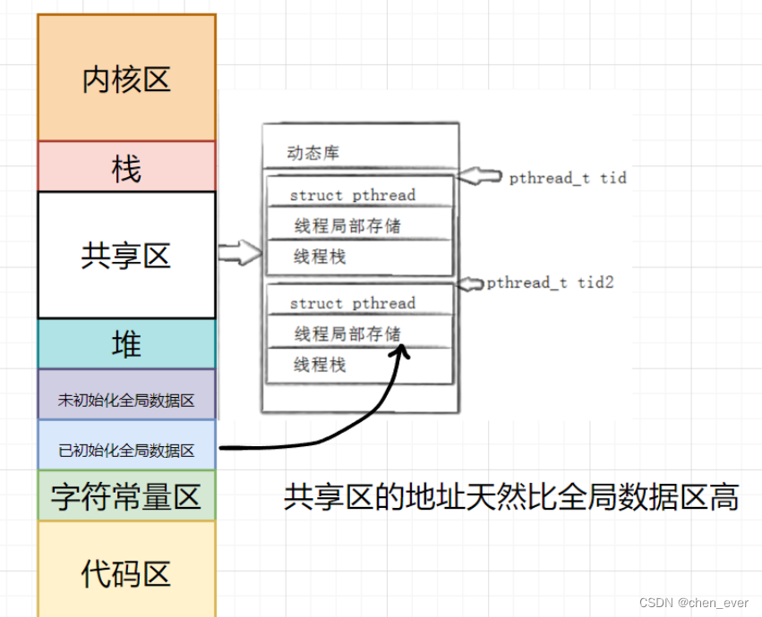
Linux线程(二)----- 线程控制
目录 前言 一、线程资源区 1.1 线程私有资源 1.2 线程共享资源 1.3 原生线程库 二、线程控制接口 2.1 线程创建 2.1.1 创建一批线程 2.2 线程等待 2.3 终止线程 2.4 线程实战 2.5 其他接口 2.5.1 关闭线程 2.5.2 获取线程ID 2.5.3 线程分离 三、深入理解线程 …...

Linux 内核irq_stack遍历
环境Centos 4.18.0-80.el8.x86_64 一、x86架构堆栈类型说明 https://www.kernel.org/doc/Documentation/x86/kernel-stacks int get_stack_info(unsigned long *stack, struct task_struct *task,struct stack_info *info, unsigned long *visit_mask) {if (!stack)goto unk…...

GIT问题记录
一、 1.Gitee相关 复现步骤:自己在gitee上使用WEB解决冲突,本地未拉取最新的origin分支,然后本地也做了其他的修改,然后commit并且push,push时候报错,本地分支不干净 尝试拉取origin的最新内容ÿ…...

AzerothCore安装记录
尝试在FreeBSD系统下安装AzerothCore 首先安装相关软件 pkg install cmake mysql80-server boost-all装完mysql之后提示: MySQL80 has a default /usr/local/etc/mysql/my.cnf, remember to replace it with your own or set mysql_optfile"$YOUR_CNF_FILE i…...

Infineon_TC264智能车代码初探及C语言深度学习(一)
本篇文章记录我在智能车竞赛中,对 Infineon_TC264 这款芯片的底层库函数的学习分析。通过深入地对其库函数进行分析,C语言深入的知识得以再次在编程中呈现和运用。故觉得很有必要在此进行记录一下。 目录 编辑 一、代码段 1、枚举类型 2、结构体 …...
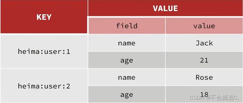
[Redis]——初识Redis
一、Redis为非关系型数据库 ❓我们常见的MySQL、SQLServer都是关系型数据库,那他们之间有什么区别与联系呢? 📕关系型数据库与非关系型数据库的区别(面试题) 解释: SQL数据库中的表是有结构的,包…...

YTM32的同步串行通信外设SPI外设详解(Master Part)
YTM32的同步串行通信外设SPI外设详解(Master Part) 文章目录 YTM32的同步串行通信外设SPI外设详解(Master Part)IntroductionFeatures引脚信号时钟源其它不常用功能 Pricinple & Mechinism基于FIFO的命令和数据管理机制锁定配…...
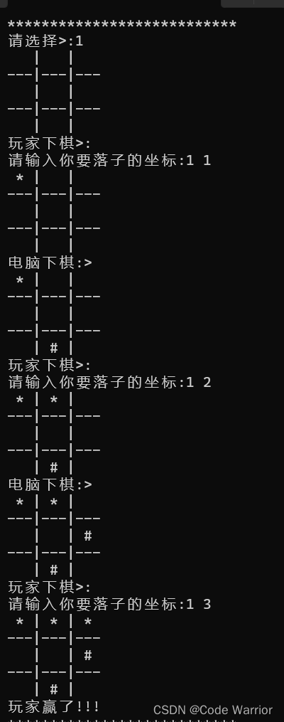
【C语言】三子棋
前言: 三子棋是一种民间传统游戏,又叫九宫棋、圈圈叉叉棋、一条龙、井字棋等。游戏规则是双方对战,双方依次在9宫格棋盘上摆放棋子,率先将自己的三个棋子走成一条线就视为胜利。但因棋盘太小,三子棋在很多时候会出现和…...
Web组态可视化编辑器 快速绘制组态
随着工业智能制造的发展,工业企业对设备可视化、远程运维的需求日趋强烈,传统的单机版组态软件已经不能满足越来越复杂的控制需求,那么实现Web组态可视化界面成为了主要的技术路径。 行业痛点 对于软件服务商来说,将单机版软件转变…...
WebServer -- 注册登录
目录 🍉整体内容 🌼流程图 🎂载入数据库表 提取用户名和密码 🚩同步线程登录注册 补充解释 代码 😘页面跳转 补充解释 代码 🍉整体内容 概述 TinyWebServer 中,使用数据库连接池实现…...

C3_W2_Collaborative_RecSys_Assignment_吴恩达_中英_Pytorch
Practice lab: Collaborative Filtering Recommender Systems(实践实验室:协同过滤推荐系统) In this exercise, you will implement collaborative filtering to build a recommender system for movies. 在本次实验中,你将实现协同过滤来构建一个电影推荐系统。 …...

Elasticsearch使用function_score查询酒店和排序
需求 基于用户地理位置,对酒店做简单的排序,非个性化的推荐。酒店评分包含以下: 酒店类型(依赖用户历史订单数据):希望匹配出更加符合用户使用的酒店类型酒店评分:评分高的酒店用户体验感好ge…...
iOS消息发送流程
Objc的方法调用基于消息发送机制。即Objc中的方法调用,在底层实际都是通过调用objc_msgSend方法向对象消息发送消息来实现的。在iOS中, 实例对象的方法主要存储在类的方法列表中,类方法则是主要存储在原类中。 向对象发送消息,核心…...
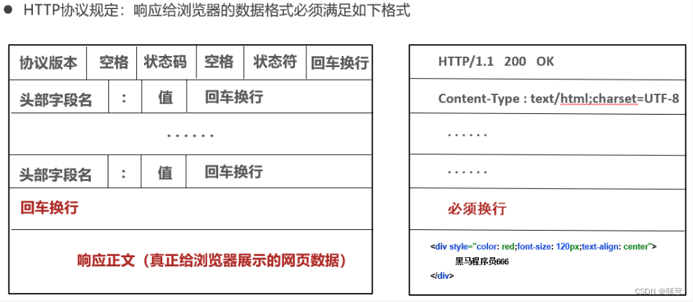
【接口测试】常见HTTP面试题
目录 HTTP GET 和 POST 的区别 GET 和 POST 方法都是安全和幂等的吗 接口幂等实现方式 说说 post 请求的几种参数格式是什么样的? HTTP特性 HTTP(1.1) 的优点有哪些? HTTP(1.1) 的缺点有哪些&#x…...
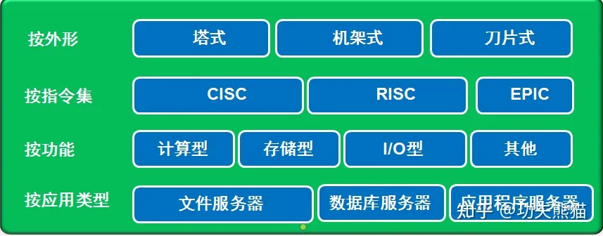
服务器硬件基础知识
1. 服务器分类 服务器分类 服务器的分类没有一个统一的标准。 从多个多个维度来看服务器的分类可以加深我们对各种服务器的认识。 N.B. CISC: complex instruction set computing 复杂指令集计算 RISC: reduced instruction set computer 精简指令集计算 EPIC: explicitly p…...
matlab实现层次聚类与k-均值聚类算法
1. 原理 1.层次聚类:通过计算两类数据点间的相似性,对所有数据点中最为相似的两个数据点进行组合,并反复迭代这一过程并生成聚类树 2.k-means聚类:在数据集中根据一定策略选择K个点作为每个簇的初始中心,然后将数据划…...

FastbootEnhance 专业指南:掌握Windows平台Android设备底层管理核心技术
FastbootEnhance 专业指南:掌握Windows平台Android设备底层管理核心技术 【免费下载链接】FastbootEnhance A user-friendly Fastboot ToolBox & Payload Dumper for Windows 项目地址: https://gitcode.com/gh_mirrors/fa/FastbootEnhance FastbootEnha…...

利用LFM2.5-1.2B-Thinking-GGUF构建智能知识库问答:基于本地文档的精准回答
利用LFM2.5-1.2B-Thinking-GGUF构建智能知识库问答:基于本地文档的精准回答 1. 企业知识管理的痛点与解决方案 在日常工作中,企业员工经常需要查阅大量内部文档——产品手册、技术规范、公司制度等。传统的关键词搜索往往效率低下,要么返回…...
)
OpenStack Dashboard安装后访问不了?排查这5个坑(从ALLOWED_HOSTS到WSGI配置)
OpenStack Dashboard安装后访问不了?排查这5个坑(从ALLOWED_HOSTS到WSGI配置) 刚部署完OpenStack Dashboard,却发现浏览器始终打不开页面?这种挫败感我太熟悉了。去年在客户现场部署时,我也曾对着404错误页…...

Vibe Coding:用“氛围感”重塑编程
Vibe Coding(氛围编程)是由OpenAI联合创始人Andrej Karpathy于2025年初提出的编程新范式,核心是通过自然语言描述需求,由AI生成代码,开发者角色从"编码者"转变为"需求引导者"和"结果优化者&q…...

千问3.5-2B部署案例:CSDN GPU平台一键启用,7860端口服务管理全命令解析
千问3.5-2B部署案例:CSDN GPU平台一键启用,7860端口服务管理全命令解析 1. 千问3.5-2B模型简介 千问3.5-2B是Qwen系列中的小型视觉语言模型,它能够同时理解图片内容和处理自然语言。这个模型特别适合需要结合视觉和语言理解的应用场景。 与…...

字符串拼接用“+”还是 StringBuilder?别再凭感觉写了辜
前言 Kubernetes 本身并不复杂,是我们把它搞复杂的。无论是刻意为之还是那种虽然出于好意却将优雅的原语堆砌成 鲁布戈德堡机械 的狂热。平台最初提供的 ReplicaSets、Services、ConfigMaps,这些基础组件简单直接,甚至显得有些枯燥。但后来我…...

AI软件研发成本飙升的真相:3个被忽视的隐性成本源,今天不查明天多烧47%预算!
第一章:AI原生软件研发成本优化实战技巧 2026奇点智能技术大会(https://ml-summit.org) AI原生软件的研发成本常被模型训练开销主导,但实际可观测的浪费更多来自推理服务冗余、提示工程低效、以及缺乏细粒度资源编排。聚焦可落地的降本路径,…...

N20 设备驱动程序
一、驱动程序驱动 内核的一部分,操作系统把硬件 “关起来”,只让驱动碰,应用程序只能通过系统调用访问。因为硬件不能直接给应用程序用,必须由操作系统统一管理,驱动就是操作系统跟硬件之间的翻译官。为应用层提供设备的操作方法…...

第三十三课:LIF神经元模型与SpikingJelly实战解析
1. LIF神经元模型:从生物启发的数学原理说起 第一次看到LIF(Leaky Integrate-and-Fire)神经元时,我脑海中浮现的是中学物理课上那个总在漏电的电容器。这种神经元模型之所以被称为"漏电积分放电",正是因为它…...

从0到1打造完美PRD:这10个细节让你的需求文档更专业
从0到1打造完美PRD:这10个细节让你的需求文档更专业 在跨部门协作的产品开发中,一份优秀的PRD(产品需求文档)如同航海图,既能指引团队方向,又能规避潜在风险。但现实中,许多产品经理的文档常陷入…...