C3_W2_Collaborative_RecSys_Assignment_吴恩达_中英_Pytorch
 Practice lab: Collaborative Filtering Recommender Systems(实践实验室:协同过滤推荐系统)
In this exercise, you will implement collaborative filtering to build a recommender system for movies.
在本次实验中,你将实现协同过滤来构建一个电影推荐系统。
 Outline
- 1 - Notation(注释)
- 2 - Recommender Systems(推荐系统)
- 3 - Movie ratings dataset(电影评分数据集)
- 4 - Collaborative filtering learning algorithm(协同过滤学习算法)
- 4.1 Collaborative filtering cost function(协同过滤代价函数)
- Exercise 1
- 4.1 Collaborative filtering cost function(协同过滤代价函数)
- 5 - Learning movie recommendations(学习电影推荐)
- 6 - Recommendations(推荐)
- 7 - Congratulations!
 Packages
We will use the now familiar NumPy and Tensorflow Packages.
我们将使用熟悉的NumPy和Tensorflow包。
import numpy as np
import tensorflow as tf
from tensorflow import keras
from recsys_utils import *
1 - Notation(注释)
| General Notation | Description | Python (if any) |
|---|---|---|
| r ( i , j ) r(i,j) r(i,j) | scalar; = 1 if user j rated game i = 0 otherwise | |
| y ( i , j ) y(i,j) y(i,j) | scalar; = rating given by user j on game i (if r(i,j) = 1 is defined) | |
| w ( j ) \mathbf{w}^{(j)} w(j) | vector; parameters for user j | |
| b ( j ) b^{(j)} b(j) | scalar; parameter for user j | |
| x ( i ) \mathbf{x}^{(i)} x(i) | vector; feature ratings for movie i | |
| n u n_u nu | number of users | num_users |
| n m n_m nm | number of movies | num_movies |
| n n n | number of features | num_features |
| X \mathbf{X} X | matrix of vectors x ( i ) \mathbf{x}^{(i)} x(i) | X |
| W \mathbf{W} W | matrix of vectors w ( j ) \mathbf{w}^{(j)} w(j) | W |
| b \mathbf{b} b | vector of bias parameters b ( j ) b^{(j)} b(j) | b |
| R \mathbf{R} R | matrix of elements r ( i , j ) r(i,j) r(i,j) | R |
 2 - Recommender Systems(推荐系统)
In this lab, you will implement the collaborative filtering learning algorithm and apply it to a dataset of movie ratings.
The goal of a collaborative filtering recommender system is to generate two vectors: For each user, a parameter vector that embodies the movie tastes of a user. For each movie, a feature vector of the same size which embodies some description of the movie. The dot product of the two vectors plus the bias term should produce an estimate of the rating the user might give to that movie.
在此实验中,您将实现协同过滤学习算法,并将其应用于电影评分的数据集。
协同过滤推荐系统的目标是生成两个向量:对于每个用户,一个参数向量,它表达了用户的观影喜好。对于每部电影,一个特征向量的大小相同,它表达了有关电影的一些描述。两个向量的点积加上偏置项应该产生一个估计值,即用户可能会给该电影打多少分。
The diagram below details how these vectors are learned.
下图详细说明了如何学习这些向量。

Existing ratings are provided in matrix form as shown. Y Y Y contains ratings; 0.5 to 5 inclusive in 0.5 steps. 0 if the movie has not been rated. R R R has a 1 where movies have been rated. Movies are in rows, users in columns. Each user has a parameter vector w u s e r w^{user} wuser and bias. Each movie has a feature vector x m o v i e x^{movie} xmovie. These vectors are simultaneously learned by using the existing user/movie ratings as training data. One training example is shown above: w ( 1 ) ⋅ x ( 1 ) + b ( 1 ) = 4 \mathbf{w}^{(1)} \cdot \mathbf{x}^{(1)} + b^{(1)} = 4 w(1)⋅x(1)+b(1)=4. It is worth noting that the feature vector x m o v i e x^{movie} xmovie must satisfy all the users while the user vector w u s e r w^{user} wuser must satisfy all the movies. This is the source of the name of this approach - all the users collaborate to generate the rating set.
现有额定值以矩阵形式提供,如下所示。 Y Y Y包含评级;0.5到5,包括0.5个步骤。0表示如果电影没有评级。 R R R有一个1表示电影的评级。电影以行表示,用户以列表示。每个用户都有一个参数向量 w u s e r w^{user} wuser和偏差。每部电影有一个特征向量 x m o v i e x^{movie} xmovie。这些向量通过使用现有的用户/电影评分作为训练数据来同时学习。上面显示了一个训练示例: w ( 1 ) ⋅ x ( 1 ) + b ( 1 ) = 4 \mathbf{w}^{(1)} \cdot \mathbf{x}^{(1)} + b^{(1)} = 4 w(1)⋅x(1)+b(1)=4。值得注意的是,特征向量 x m o v i e x^{movie} xmovie必须满足所有用户,而用户向量 w u s e r w^{user} wuser必须满足所有电影。这是该方法名称的来源——所有用户协作生成评级集。

Once the feature vectors and parameters are learned, they can be used to predict how a user might rate an unrated movie. This is shown in the diagram above. The equation is an example of predicting a rating for user one on movie zero.
一旦学习了特征向量和参数,就可以用来预测用户对未评级的电影的评分。这在上面给出的图表中显示。方程是一个预测用户对电影0的评分的示例。
In this exercise, you will implement the function cofiCostFunc that computes the collaborative filtering
objective function. After implementing the objective function, you will use a TensorFlow custom training loop to learn the parameters for collaborative filtering. The first step is to detail the data set and data structures that will be used in the lab.
在本次练习中,您将实现函数cofiCostFunc,该函数计算协同过滤的目标函数。实现目标函数后,您将使用TensorFlow自定义训练循环来学习协同过滤的参数。第一步是详细说明将在实验室中使用的数据集和数据结构。
 3 - Movie ratings dataset(电影评分数据集)
The data set is derived from the MovieLens “ml-latest-small” dataset.
[F. Maxwell Harper and Joseph A. Konstan. 2015. The MovieLens Datasets: History and Context. ACM Transactions on Interactive Intelligent Systems (TiiS) 5, 4: 19:1–19:19. https://doi.org/10.1145/2827872]
The original dataset has 9000 movies rated by 600 users. The dataset has been reduced in size to focus on movies from the years since 2000. This dataset consists of ratings on a scale of 0.5 to 5 in 0.5 step increments. The reduced dataset has n u = 443 n_u = 443 nu=443 users, and n m = 4778 n_m= 4778 nm=4778 movies.
原始数据集有600个用户评分的9000部电影。该数据集的大小已经缩小,以关注2000年以来的电影。该数据集由0.5到5的评分组成,以0.5步为增量。约简后的数据集 n u = 443 n_u = 443 nu=443 users, n m = 4778 n_m= 4778 nm=4778 movies。
Below, you will load the movie dataset into the variables Y Y Y and R R R.
下面,你将加载电影数据集到变量 Y Y Y和 R R R中。
The matrix Y Y Y (a n m × n u n_m \times n_u nm×nu matrix) stores the ratings y ( i , j ) y^{(i,j)} y(i,j). The matrix R R R is an binary-valued indicator matrix, where R ( i , j ) = 1 R(i,j) = 1 R(i,j)=1 if user j j j gave a rating to movie i i i, and R ( i , j ) = 0 R(i,j)=0 R(i,j)=0 otherwise.
矩阵 Y Y Y(一个 n m × n u n_m \times n_u nm×nu矩阵)存储评分 y ( i , j ) y^{(i,j)} y(i,j)。矩阵 R R R是一个二进制值的指示矩阵,其中 R ( i , j ) = 1 R(i,j) = 1 R(i,j)=1如果用户 j j j给电影 i i i评分,否则 R ( i , j ) = 0 R(i,j)=0 R(i,j)=0。
Throughout this part of the exercise, you will also be working with the
在本部分练习中,您还将使用
matrices, X \mathbf{X} X, W \mathbf{W} W and b \mathbf{b} b:
X = [ − − − ( x ( 0 ) ) T − − − − − − ( x ( 1 ) ) T − − − ⋮ − − − ( x ( n m − 1 ) ) T − − − ] , W = [ − − − ( w ( 0 ) ) T − − − − − − ( w ( 1 ) ) T − − − ⋮ − − − ( w ( n u − 1 ) ) T − − − ] , b = [ b ( 0 ) b ( 1 ) ⋮ b ( n u − 1 ) ] \mathbf{X} = \begin{bmatrix} --- (\mathbf{x}^{(0)})^T --- \\ --- (\mathbf{x}^{(1)})^T --- \\ \vdots \\ --- (\mathbf{x}^{(n_m-1)})^T --- \\ \end{bmatrix} , \quad \mathbf{W} = \begin{bmatrix} --- (\mathbf{w}^{(0)})^T --- \\ --- (\mathbf{w}^{(1)})^T --- \\ \vdots \\ --- (\mathbf{w}^{(n_u-1)})^T --- \\ \end{bmatrix},\quad \mathbf{ b} = \begin{bmatrix} b^{(0)} \\ b^{(1)} \\ \vdots \\ b^{(n_u-1)} \\ \end{bmatrix}\quad X= −−−(x(0))T−−−−−−(x(1))T−−−⋮−−−(x(nm−1))T−−− ,W= −−−(w(0))T−−−−−−(w(1))T−−−⋮−−−(w(nu−1))T−−− ,b= b(0)b(1)⋮b(nu−1)
The i i i-th row of X \mathbf{X} X corresponds to thefeature vector x ( i ) x^{(i)} x(i) for the i i i-th movie, and the j j j-th row of W \mathbf{W} W corresponds to one parameter vector w ( j ) \mathbf{w}^{(j)} w(j), for the j j j -th user. Both x ( i ) x^{(i)} x(i) and w ( j ) \mathbf{w}^{(j)} w(j) are n n n-dimensional vectors. For the purposes of this exercise, you will use n = 10 n=10 n=10, and therefore, x ( i ) \mathbf{x}^{(i)} x(i) and w ( j ) \mathbf{w}^{(j)} w(j) have 10 elements. Correspondingly, X \mathbf{X} X is a n m × 10 n_m \times 10 nm×10 matrix and W \mathbf{W} W is a n u × 10 n_u \times 10 nu×10 matrix.
X \mathbf{X} X的 i i i-第一行对应于特征向量 x ( i ) x^{(i)} x(i)表示第i部电影, j j j表示第j行 W \mathbf{W} W 对应一个参数向量 w ( j ) \mathbf{w}^{(j)} w(j),对于第j个用户。 x ( i ) x^{(i)} x(i)和 w ( j ) \mathbf{w}^{(j)} w(j)都是 n n n维向量。为了本练习的目的,您将使用 n = 10 n=10 n=10,因此, x ( i ) \mathbf{x}^{(i)} x(i)和 w ( j ) \mathbf{w}^{(j)} w(j)有10个元素。相应地, X \mathbf{X} X是一个 n m × 10 n_m \times 10 nm×10矩阵, W \mathbf{W} W是一个 n u × 10 n_u \times 10 nu×10矩阵。
We will start by loading the movie ratings dataset to understand the structure of the data.
我们将从加载电影评分数据集开始,以了解数据结构。
We will load Y Y Y and R R R with the movie dataset.
我们将使用电影数据集加载 Y Y Y和 R R R。
We’ll also load X \mathbf{X} X, W \mathbf{W} W, and b \mathbf{b} b with pre-computed values. These values will be learned later in the lab, but we’ll use pre-computed values to develop the cost model.
我们还会加载 X \mathbf{X} X, W \mathbf{W} W和 b \mathbf{b} b,使用预先计算的值。这些值将在实验后期学习,但我们使用预先计算的值来发展成本模型。
#Load data
X, W, b, num_movies, num_features, num_users = load_precalc_params_small()
Y, R = load_ratings_small()print("Y", Y.shape, "R", R.shape)
print("X", X.shape)
print("W", W.shape)
print("b", b.shape)
print("num_features", num_features)
print("num_movies",   num_movies)
print("num_users",    num_users)
Y (4778, 443) R (4778, 443)
X (4778, 10)
W (443, 10)
b (1, 443)
num_features 10
num_movies 4778
num_users 443
#  From the matrix, we can compute statistics like average rating.
tsmean =  np.mean(Y[0, R[0, :].astype(bool)])
print(f"Average rating for movie 1 : {tsmean:0.3f} / 5" )
Average rating for movie 1 : 3.400 / 5
 4 - Collaborative filtering learning algorithm(协同过滤算法)
Now, you will begin implementing the collaborative filtering learning
algorithm. You will start by implementing the objective function.
现在,你将开始实现协同过滤学习算法。你将从实现目标函数开始。
The collaborative filtering algorithm in the setting of movie recommendations considers a set of n n n-dimensional parameter vectors
电影推荐设置中的协同过滤算法考虑一组n维参数向量
x ( 0 ) , . . . , x ( n m − 1 ) \mathbf{x}^{(0)},...,\mathbf{x}^{(n_m-1)} x(0),...,x(nm−1), w ( 0 ) , . . . , w ( n u − 1 ) \mathbf{w}^{(0)},...,\mathbf{w}^{(n_u-1)} w(0),...,w(nu−1) and b ( 0 ) , . . . , b ( n u − 1 ) b^{(0)},...,b^{(n_u-1)} b(0),...,b(nu−1)
where the model predicts the rating for movie i i i by user j j j as
该模型预测用户 j j j as对电影 i i i的评分
y ( i , j ) = w ( j ) ⋅ x ( i ) + b ( i ) y^{(i,j)} = \mathbf{w}^{(j)}\cdot \mathbf{x}^{(i)} + b^{(i)} y(i,j)=w(j)⋅x(i)+b(i)
Given a dataset that consists of a set of ratings produced by some users on some movies, you wish to learn the parameter vectors x ( 0 ) , . . . , x ( n m − 1 ) , w ( 0 ) , . . . , w ( n u − 1 ) \mathbf{x}^{(0)},...,\mathbf{x}^{(n_m-1)}, \mathbf{w}^{(0)},...,\mathbf{w}^{(n_u-1)} x(0),...,x(nm−1),w(0),...,w(nu−1) and b ( 0 ) , . . . , b ( n u − 1 ) b^{(0)},...,b^{(n_u-1)} b(0),...,b(nu−1) that produce the best fit (minimizes
the squared error).
给定一个数据集,它由一些用户对一些电影给出的评分组成,你希望学习参数向量 x ( 0 ) , . . . , x ( n m − 1 ) , w ( 0 ) , . . . , w ( n u − 1 ) \mathbf{x}^{(0)},...,\mathbf{x}^{(n_m-1)}, \mathbf{w}^{(0)},...,\mathbf{w}^{(n_u-1)} x(0),...,x(nm−1),w(0),...,w(nu−1) 和 b ( 0 ) , . . . , b ( n u − 1 ) b^{(0)},...,b^{(n_u-1)} b(0),...,b(nu−1),以产生最佳拟合(最小化平方误差)。
You will complete the code in cofiCostFunc to compute the cost function for collaborative filtering.
你将在cofiCostFunc中完成代码以计算协同过滤的成本函数。
4.1 Collaborative filtering cost function(协同过滤代价函数)
The collaborative filtering cost function is given by
协同过滤代价函数由以下公式给出:
$$J({\mathbf{x}{(0)},…,\mathbf{x}{(n_m-1)},\mathbf{w}{(0)},b{(0)},…,\mathbf{w}{(n_u-1)},b{(n_u-1)}})= \frac{1}{2}\sum_{(i,j):r(i,j)=1}(\mathbf{w}^{(j)} \cdot \mathbf{x}^{(i)} + b^{(j)} - y{(i,j)})2
+\underbrace{
\frac{\lambda}{2}
\sum_{j=0}{n_u-1}\sum_{k=0}{n-1}(\mathbf{w}{(j)}_k)2
- \frac{\lambda}{2}\sum_{i=0}{n_m-1}\sum_{k=0}{n-1}(\mathbf{x}k{(i)})2
}{regularization}
\tag{1}$$
The first summation in (1) is “for all i i i, j j j where r ( i , j ) r(i,j) r(i,j) equals 1 1 1” and could be written:
(1)中的第一个求和是“对于所有 i i i, j j j,其中 r ( i , j ) r(i,j) r(i,j)等于 1 1 1”,可以写成:
= 1 2 ∑ j = 0 n u − 1 ∑ i = 0 n m − 1 r ( i , j ) ∗ ( w ( j ) ⋅ x ( i ) + b ( j ) − y ( i , j ) ) 2 + regularization = \frac{1}{2}\sum_{j=0}^{n_u-1} \sum_{i=0}^{n_m-1}r(i,j)*(\mathbf{w}^{(j)} \cdot \mathbf{x}^{(i)} + b^{(j)} - y^{(i,j)})^2 +\text{regularization} =21j=0∑nu−1i=0∑nm−1r(i,j)∗(w(j)⋅x(i)+b(j)−y(i,j))2+regularization
You should now write cofiCostFunc (collaborative filtering cost function) to return this cost.
你现在应该编写cofiCostFunc(协同过滤代价函数)来返回这个代价。
Exercise 1
For loop Implementation(for循环实现):
Start by implementing the cost function using for loops.
首先使用for循环实现代价函数。
Consider developing the cost function in two steps. First, develop the cost function without regularization. A test case that does not include regularization is provided below to test your implementation. Once that is working, add regularization and run the tests that include regularization. Note that you should be accumulating the cost for user j j j and movie i i i only if R ( i , j ) = 1 R(i,j) = 1 R(i,j)=1.
考虑在两个步骤中实现代价函数。首先,在不包含正则化的代价函数。一个不包含正则化的测试用例是提供的,以测试你的实现。一旦它工作正常,添加正则化并运行包含正则化的测试用例。请注意,您应该只累积用户 j j j和电影 i i i的成本,如果 R ( i , j ) = 1 R(i,j)=1 R(i,j)=1。
# GRADED FUNCTION: cofi_cost_func
# UNQ_C1def cofi_cost_func(X, W, b, Y, R, lambda_):"""Returns the cost for the content-based filteringArgs:X (ndarray (num_movies,num_features)): matrix of item featuresW (ndarray (num_users,num_features)) : matrix of user parametersb (ndarray (1, num_users)            : vector of user parametersY (ndarray (num_movies,num_users)    : matrix of user ratings of moviesR (ndarray (num_movies,num_users)    : matrix, where R(i, j) = 1 if the i-th movies was rated by the j-th userlambda_ (float): regularization parameterReturns:J (float) : Cost"""nm, nu = Y.shapeJ = 0### START CODE HERE ###  for j in range(nu):w = W[j,:]b_j = b[0,j]for i in range(nm):x = X[i,:]r = R[i,j]y = Y[i,j]J += np.square(r * (np.dot(w,x) + b_j - y))  J +=lambda_ * (np.sum(np.square(W)) + np.sum(np.square(X)))J = J/2   ### END CODE HERE ### return J
# Public tests
from public_tests import *
test_cofi_cost_func(cofi_cost_func);
[92mAll tests passed!
### START CODE HERE ### for j in range(nu):for i in range(nm):### END CODE HERE ###
Here is some more details. The code below pulls out each element from the matrix before using it.
One could also reference the matrix directly.
This code does not contain regularization.
nm,nu = Y.shapeJ = 0### START CODE HERE ### for j in range(nu):w = W[j,:]b_j = b[0,j]for i in range(nm):x = y = r =J += J = J/2### END CODE HERE ### nm,nu = Y.shapeJ = 0### START CODE HERE ### for j in range(nu):w = W[j,:]b_j = b[0,j]for i in range(nm):x = X[i,:]y = Y[i,j]r = R[i,j]J += np.square(r * (np.dot(w,x) + b_j - y ) )J = J/2### END CODE HERE ###
J += lambda_* (np.sum(np.square(W)) + np.sum(np.square(X)))
# Reduce the data set size so that this runs faster
num_users_r = 4
num_movies_r = 5
num_features_r = 3X_r = X[:num_movies_r, :num_features_r]
W_r = W[:num_users_r,  :num_features_r]
b_r = b[0, :num_users_r].reshape(1,-1)
Y_r = Y[:num_movies_r, :num_users_r]
R_r = R[:num_movies_r, :num_users_r]# Evaluate cost function
J = cofi_cost_func(X_r, W_r, b_r, Y_r, R_r, 0);
print(f"Cost: {J:0.2f}")
Cost: 13.67
Expected Output (lambda = 0):
13.67 13.67 13.67.
# Evaluate cost function with regularization
J = cofi_cost_func(X_r, W_r, b_r, Y_r, R_r, 1.5)
print(f"Cost (with regularization): {J:0.2f}")
Cost (with regularization): 28.09
Expected Output:
28.09
Vectorized Implementation(向量化实现)
It is important to create a vectorized implementation to compute J J J, since it will later be called many times during optimization. The linear algebra utilized is not the focus of this series, so the implementation is provided. If you are an expert in linear algebra, feel free to create your version without referencing the code below.
创建一个矢量化实现来计算 J J J是很重要的,因为它将在优化过程中被多次调用。所使用的线性代数不是本系列的重点,因此提供了实现。如果您是线性代数方面的专家,可以随意创建自己的版本,而无需引用下面的代码。
Run the code below and verify that it produces the same results as the non-vectorized version.
运行下面的代码,并验证它产生了与非矢量化版本相同的结果。
def cofi_cost_func_v(X, W, b, Y, R, lambda_):"""Returns the cost for the content-based filteringVectorized for speed. Uses tensorflow operations to be compatible with custom training loop.Args:X (ndarray (num_movies,num_features)): matrix of item featuresW (ndarray (num_users,num_features)) : matrix of user parametersb (ndarray (1, num_users) : vector of user parametersY (ndarray (num_movies,num_users) : matrix of user ratings of moviesR (ndarray (num_movies,num_users) : matrix, where R(i, j) = 1 if the i-th movies was rated by the j-th userlambda_ (float): regularization parameterReturns:J (float) : Cost"""j = (tf.linalg.matmul(X, tf.transpose(W)) + b - Y)*RJ = 0.5 * tf.reduce_sum(j**2) + (lambda_/2) * (tf.reduce_sum(X**2) + tf.reduce_sum(W**2))return J
# Evaluate cost function
J = cofi_cost_func_v(X_r, W_r, b_r, Y_r, R_r, 0);
print(f"Cost: {J:0.2f}")# Evaluate cost function with regularization
J = cofi_cost_func_v(X_r, W_r, b_r, Y_r, R_r, 1.5);
print(f"Cost (with regularization): {J:0.2f}")
Cost: 13.67
Cost (with regularization): 28.09
Expected Output:
Cost: 13.67
Cost (with regularization): 28.09
 5 - Learning movie recommendations(学习电影推荐)
After you have finished implementing the collaborative filtering cost function, you can start training your algorithm to make movie recommendations for yourself.
在你完成协同过滤成本函数的实现后,你可以开始训练你的算法来为你制作电影推荐。
In the cell below, you can enter your own movie choices. The algorithm will then make recommendations for you! We have filled out some values according to our preferences, but after you have things working with our choices, you should change this to match your tastes.
A list of all movies in the dataset is in the file movie list.
在下面的单元格中,你可以输入你自己的电影选择。然后,算法将为你制作推荐!我们已经根据我们的喜好填写了一些值,但当你使用我们的选择时,你应该改变这些来匹配你的品味。
数据集中所有电影的列表在文件电影列表中。
movieList, movieList_df = load_Movie_List_pd()my_ratings = np.zeros(num_movies)          #  Initialize my ratings# Check the file small_movie_list.csv for id of each movie in our dataset
# For example, Toy Story 3 (2010) has ID 2700, so to rate it "5", you can set
my_ratings[2700] = 5 #Or suppose you did not enjoy Persuasion (2007), you can set
my_ratings[2609] = 2# We have selected a few movies we liked / did not like and the ratings we
# gave are as follows:
my_ratings[929]  = 5   # Lord of the Rings: The Return of the King, The
my_ratings[246]  = 3   # Shrek (2001)
my_ratings[2716] = 4   # Inception
my_ratings[1150] = 3   # Incredibles, The (2004)
my_ratings[382]  = 2   # Amelie (Fabuleux destin d'Amélie Poulain, Le)
my_ratings[366]  = 5   # Harry Potter and the Sorcerer's Stone (a.k.a. Harry Potter and the Philosopher's Stone) (2001)
my_ratings[622]  = 5   # Harry Potter and the Chamber of Secrets (2002)
my_ratings[988]  = 3   # Eternal Sunshine of the Spotless Mind (2004)
my_ratings[2925] = 1   # Louis Theroux: Law & Disorder (2008)
my_ratings[2937] = 1   # Nothing to Declare (Rien à déclarer)
my_ratings[793]  = 5   # Pirates of the Caribbean: The Curse of the Black Pearl (2003)
my_rated = [i for i in range(len(my_ratings)) if my_ratings[i] > 0]print('\nNew user ratings:\n')
for i in range(len(my_ratings)):if my_ratings[i] > 0 :print(f'Rated {my_ratings[i]} for  {movieList_df.loc[i,"title"]}')
New user ratings:Rated 3.0 for  Shrek (2001)
Rated 5.0 for  Harry Potter and the Sorcerer's Stone (a.k.a. Harry Potter and the Philosopher's Stone) (2001)
Rated 2.0 for  Amelie (Fabuleux destin d'Amélie Poulain, Le) (2001)
Rated 5.0 for  Harry Potter and the Chamber of Secrets (2002)
Rated 5.0 for  Pirates of the Caribbean: The Curse of the Black Pearl (2003)
Rated 5.0 for  Lord of the Rings: The Return of the King, The (2003)
Rated 3.0 for  Eternal Sunshine of the Spotless Mind (2004)
Rated 3.0 for  Incredibles, The (2004)
Rated 2.0 for  Persuasion (2007)
Rated 5.0 for  Toy Story 3 (2010)
Rated 4.0 for  Inception (2010)
Rated 1.0 for  Louis Theroux: Law & Disorder (2008)
Rated 1.0 for  Nothing to Declare (Rien à déclarer) (2010)
Now, let’s add these reviews to Y Y Y and R R R and normalize the ratings.
现在,让我们将这些评论添加到 Y Y Y和 R R R中,并标准化评分。
# Reload ratings and add new ratings
Y, R = load_ratings_small()
Y    = np.c_[my_ratings, Y]
R    = np.c_[(my_ratings != 0).astype(int), R]# Normalize the Dataset
Ynorm, Ymean = normalizeRatings(Y, R)
Let’s prepare to train the model. Initialize the parameters and select the Adam optimizer.
让我们准备训练模型。初始化参数并选择Adam优化器。
#  Useful Values
num_movies, num_users = Y.shape
num_features = 100# Set Initial Parameters (W, X), use tf.Variable to track these variables
tf.random.set_seed(1234) # for consistent results
W = tf.Variable(tf.random.normal((num_users,  num_features),dtype=tf.float64),  name='W')
X = tf.Variable(tf.random.normal((num_movies, num_features),dtype=tf.float64),  name='X')
b = tf.Variable(tf.random.normal((1,          num_users),   dtype=tf.float64),  name='b')# Instantiate an optimizer.
optimizer = keras.optimizers.Adam(learning_rate=1e-1)
Let’s now train the collaborative filtering model. This will learn the parameters X \mathbf{X} X, W \mathbf{W} W, and b \mathbf{b} b.
让我们现在训练协同过滤模型。这将学习参数 X , W \mathbf{X},\mathbf{W} X,W和 b \mathbf{b} b。
The operations involved in learning w w w, b b b, and x x x simultaneously do not fall into the typical ‘layers’ offered in the TensorFlow neural network package. Consequently, the flow used in Course 2: Model, Compile(), Fit(), Predict(), are not directly applicable. Instead, we can use a custom training loop.
同时学习 w w w, b b b和 x x x所涉及的操作不属于TensorFlow神经网络包中提供的典型“层”。因此,课程2中使用的流程:Model、Compile()、Fit()、Predict()并不直接适用。相反,我们可以使用定制的训练循环。
Recall from earlier labs the steps of gradient descent.
回想一下之前的实验中关于梯度下降的步骤。
- repeat until convergence(重复直到收敛):
- compute forward pass(计算前向传播)
- compute the derivatives of the loss relative to parameters(计算相对于参数的损失函数的导数)
- update the parameters using the learning rate and the computed derivatives(使用学习率和计算出的导数更新参数)
TensorFlow has the marvelous capability of calculating the derivatives for you. This is shown below. Within the tf.GradientTape() section, operations on Tensorflow Variables are tracked. When tape.gradient() is later called, it will return the gradient of the loss relative to the tracked variables. The gradients can then be applied to the parameters using an optimizer.
TensorFlow具有神奇的 capability,可以为您计算导数。这是下面显示的。在tf.GradientTape()部分,跟踪Tensorflow Variables的操作。当稍后的tape.gradient()被调用时,它将返回相对于跟踪变量的损失函数的梯度。这些梯度可以随后应用于使用优化器的参数。
This is a very brief introduction to a useful feature of TensorFlow and other machine learning frameworks. Further information can be found by investigating “custom training loops” within the framework of interest.
这是对TensorFlow和其他机器学习框架的一个有用特性的非常简短的介绍。通过在感兴趣的框架内调查“自定义训练循环”可以找到进一步的信息。。
iterations = 200
lambda_ = 1
for iter in range(iterations):# Use TensorFlow’s GradientTape# to record the operations used to compute the cost with tf.GradientTape() as tape:# Compute the cost (forward pass included in cost)cost_value = cofi_cost_func_v(X, W, b, Ynorm, R, lambda_)# Use the gradient tape to automatically retrieve# the gradients of the trainable variables with respect to the lossgrads = tape.gradient( cost_value, [X,W,b] )# Run one step of gradient descent by updating# the value of the variables to minimize the loss.optimizer.apply_gradients( zip(grads, [X,W,b]) )# Log periodically.if iter % 20 == 0:print(f"Training loss at iteration {iter}: {cost_value:0.1f}")
Training loss at iteration 0: 2321158.0
Training loss at iteration 20: 136165.9
Training loss at iteration 40: 51862.0
Training loss at iteration 60: 24597.9
Training loss at iteration 80: 13629.8
Training loss at iteration 100: 8487.3
Training loss at iteration 120: 5807.5
Training loss at iteration 140: 4311.5
Training loss at iteration 160: 3435.2
Training loss at iteration 180: 2902.1
6 - Recommendations(推荐)
Below, we compute the ratings for all the movies and users and display the movies that are recommended. These are based on the movies and ratings entered as my_ratings[] above. To predict the rating of movie i i i for user j j j, you compute w ( j ) ⋅ x ( i ) + b ( j ) \mathbf{w}^{(j)} \cdot \mathbf{x}^{(i)} + b^{(j)} w(j)⋅x(i)+b(j). This can be computed for all ratings using matrix multiplication.
下面,我们计算所有电影的评分,并显示推荐的电影。这些是基于上面输入的my_ratings[]的电影和评分。为了预测用户 j j j对电影 i i i的评分,你可以计算 w ( j ) ⋅ x ( i ) + b ( j ) \mathbf{w}^{(j)} \cdot \mathbf{x}^{(i)} + b^{(j)} w(j)⋅x(i)+b(j)。可以使用矩阵乘法计算所有评分的预测。
# Make a prediction using trained weights and biases
p = np.matmul(X.numpy(), np.transpose(W.numpy())) + b.numpy()#restore the mean
pm = p + Ymeanmy_predictions = pm[:,0]# sort predictions
ix = tf.argsort(my_predictions, direction='DESCENDING')for i in range(17):j = ix[i]if j not in my_rated:print(f'Predicting rating {my_predictions[j]:0.2f} for movie {movieList[j]}')print('\n\nOriginal vs Predicted ratings:\n')
for i in range(len(my_ratings)):if my_ratings[i] > 0:print(f'Original {my_ratings[i]}, Predicted {my_predictions[i]:0.2f} for {movieList[i]}')
Predicting rating 4.51 for movie Lord of the Rings: The Two Towers, The (2002)
Predicting rating 4.44 for movie Dark Knight Rises, The (2012)
Predicting rating 4.39 for movie Particle Fever (2013)
Predicting rating 4.39 for movie Eichmann (2007)
Predicting rating 4.39 for movie Battle Royale 2: Requiem (Batoru rowaiaru II: Chinkonka) (2003)
Predicting rating 4.39 for movie Into the Abyss (2011)
Predicting rating 4.37 for movie My Sassy Girl (Yeopgijeogin geunyeo) (2001)
Predicting rating 4.37 for movie Bitter Lake (2015)
Predicting rating 4.37 for movie L.A. Slasher (2015)
Predicting rating 4.36 for movie Rivers and Tides (2001)
Predicting rating 4.36 for movie Loving Vincent (2017)
Predicting rating 4.36 for movie My Love (2006)Original vs Predicted ratings:Original 3.0, Predicted 3.05 for Shrek (2001)
Original 5.0, Predicted 4.80 for Harry Potter and the Sorcerer's Stone (a.k.a. Harry Potter and the Philosopher's Stone) (2001)
Original 2.0, Predicted 2.10 for Amelie (Fabuleux destin d'Amélie Poulain, Le) (2001)
Original 5.0, Predicted 4.83 for Harry Potter and the Chamber of Secrets (2002)
Original 5.0, Predicted 4.84 for Pirates of the Caribbean: The Curse of the Black Pearl (2003)
Original 5.0, Predicted 4.86 for Lord of the Rings: The Return of the King, The (2003)
Original 3.0, Predicted 3.02 for Eternal Sunshine of the Spotless Mind (2004)
Original 3.0, Predicted 3.10 for Incredibles, The (2004)
Original 2.0, Predicted 2.09 for Persuasion (2007)
Original 5.0, Predicted 4.73 for Toy Story 3 (2010)
Original 4.0, Predicted 3.94 for Inception (2010)
Original 1.0, Predicted 1.38 for Louis Theroux: Law & Disorder (2008)
Original 1.0, Predicted 1.24 for Nothing to Declare (Rien à déclarer) (2010)
In practice, additional information can be utilized to enhance our predictions. Above, the predicted ratings for the first few hundred movies lie in a small range. We can augment the above by selecting from those top movies, movies that have high average ratings and movies with more than 20 ratings. This section uses a Pandas data frame which has many handy sorting features.
在实践中,可以利用额外的信息来增强我们的预测。上面,对前几百部电影的预测评分在一个小范围内。我们可以通过从那些顶级电影、平均评分高的电影和评分超过20的电影中选择电影来增强上述内容。本节使用一个Pandas数据框架,它有许多方便的排序特性。
filter=(movieList_df["number of ratings"] > 20)
movieList_df["pred"] = my_predictions
movieList_df = movieList_df.reindex(columns=["title", "number of ratings","mean rating",  "pred"])
movieList_df.loc[ix[:300]].loc[filter].sort_values("mean rating", ascending=False)
| title | number of ratings | mean rating | pred | |
|---|---|---|---|---|
| 929 | Lord of the Rings: The Return of the King, The... | 185 | 4.118919 | 4.856171 |
| 2700 | Toy Story 3 (2010) | 55 | 4.109091 | 4.726026 |
| 393 | Lord of the Rings: The Fellowship of the Ring,... | 198 | 4.106061 | 4.171893 |
| 2716 | Inception (2010) | 143 | 4.066434 | 3.940508 |
| 848 | Lost in Translation (2003) | 74 | 4.033784 | 3.915533 |
| 653 | Lord of the Rings: The Two Towers, The (2002) | 188 | 4.021277 | 4.505254 |
| 1122 | Shaun of the Dead (2004) | 77 | 4.006494 | 4.066710 |
| 3083 | Dark Knight Rises, The (2012) | 76 | 3.993421 | 4.439322 |
| 2804 | Harry Potter and the Deathly Hallows: Part 1 (... | 47 | 3.989362 | 4.096199 |
| 1771 | Casino Royale (2006) | 81 | 3.944444 | 3.966460 |
| 2649 | How to Train Your Dragon (2010) | 53 | 3.943396 | 4.303658 |
| 174 | Traffic (2000) | 70 | 3.900000 | 4.001369 |
| 2455 | Harry Potter and the Half-Blood Prince (2009) | 58 | 3.887931 | 4.062298 |
| 2523 | Zombieland (2009) | 53 | 3.877358 | 4.025288 |
| 361 | Monsters, Inc. (2001) | 132 | 3.871212 | 3.967351 |
| 3014 | Avengers, The (2012) | 69 | 3.869565 | 4.022406 |
| 1930 | Harry Potter and the Order of the Phoenix (2007) | 58 | 3.862069 | 4.000611 |
| 151 | Crouching Tiger, Hidden Dragon (Wo hu cang lon... | 110 | 3.836364 | 3.875230 |
| 793 | Pirates of the Caribbean: The Curse of the Bla... | 149 | 3.778523 | 4.838517 |
| 366 | Harry Potter and the Sorcerer's Stone (a.k.a. ... | 107 | 3.761682 | 4.803115 |
| 622 | Harry Potter and the Chamber of Secrets (2002) | 102 | 3.598039 | 4.831402 |
 7 - Congratulations!
You have implemented a useful recommender system!
你已经实现了一个有用的推荐系统!
使用Pytorch实现梯度更新,获得更好推荐
首先导入我们需要的包
import torch
import numpy as np
from torch.autograd import Variable
from recsys_utils import *
加载数据集
movieList, movieList_df = load_Movie_List_pd()
X, W, b, num_movies, num_features, num_users = load_precalc_params_small()
定义协同过滤代价函数
def cofi_cost_func_v(X,W,b,Y,R,lambda_):j = (torch.matmul(X,torch.transpose(W,0,1)) + b - Y)*Rj = 0.5 * torch.sum(j**2) + (lambda_/2) * (torch.sum(W**2) + torch.sum(X**2))return j
my_ratings = np.zeros(num_movies)          # 初始化我的喜好程度# 检查文件small_movie_list.csv以获取数据集中每部电影的id
# 例如,《玩具总动员3》(2010)的ID为2700,所以你可以设置为“5”
my_ratings[2700] = 5 #或者假设你不喜欢劝导(2007),你可以设置
my_ratings[2609] = 2# 我们选择了一些我们喜欢/不喜欢的电影和我们的评级
# gave are as follows:
my_ratings[929]  = 5   # Lord of the Rings: The Return of the King, The
my_ratings[246]  = 3   # Shrek (2001)
my_ratings[2716] = 4   # Inception
my_ratings[1150] = 3   # Incredibles, The (2004)
my_ratings[382]  = 2   # Amelie (Fabuleux destin d'Amélie Poulain, Le)
my_ratings[366]  = 5   # Harry Potter and the Sorcerer's Stone (a.k.a. Harry Potter and the Philosopher's Stone) (2001)
my_ratings[622]  = 5   # Harry Potter and the Chamber of Secrets (2002)
my_ratings[988]  = 3   # Eternal Sunshine of the Spotless Mind (2004)
my_ratings[2925] = 1   # Louis Theroux: Law & Disorder (2008)
my_ratings[2937] = 1   # Nothing to Declare (Rien à déclarer)
my_ratings[793]  = 5   # Pirates of the Caribbean: The Curse of the Black Pearl (2003)
my_rated = [i for i in range(len(my_ratings)) if my_ratings[i] > 0]print('\nNew user ratings:\n')
for i in range(len(my_ratings)):if my_ratings[i] > 0 :print(f'Rated {my_ratings[i]} for  {movieList_df.loc[i,"title"]}')
New user ratings:Rated 3.0 for  Shrek (2001)
Rated 5.0 for  Harry Potter and the Sorcerer's Stone (a.k.a. Harry Potter and the Philosopher's Stone) (2001)
Rated 2.0 for  Amelie (Fabuleux destin d'Amélie Poulain, Le) (2001)
Rated 5.0 for  Harry Potter and the Chamber of Secrets (2002)
Rated 5.0 for  Pirates of the Caribbean: The Curse of the Black Pearl (2003)
Rated 5.0 for  Lord of the Rings: The Return of the King, The (2003)
Rated 3.0 for  Eternal Sunshine of the Spotless Mind (2004)
Rated 3.0 for  Incredibles, The (2004)
Rated 2.0 for  Persuasion (2007)
Rated 5.0 for  Toy Story 3 (2010)
Rated 4.0 for  Inception (2010)
Rated 1.0 for  Louis Theroux: Law & Disorder (2008)
Rated 1.0 for  Nothing to Declare (Rien à déclarer) (2010)
我们先介绍如下的函数:
torch.randn: 产生一个服从标准整正态分布的张量,张量内数据均值为0,方差为1,即为高斯白噪声。- torch.normal:torch.randn(mean=0, std=1, size): 产生一个服从离散正态分布的张量随机数,可以指定均值和标准差。其中,标准差std是一个张量包含每个输出元素相关的正态分布标准差
autograd.Variable: 是包的核心类,包装张量,支持几乎所有操作,并且能够跟踪和计算梯度。可以通过调用.backword()方法来自动计算所有梯度,并且可以通过.data属性访问原始张量。该变量的梯度会被累计到.grad上去requires_grad = True该函数的作用是设置一个变量,当该变量被设置为True时,该变量将自动跟踪梯度。
Y,R = load_ratings_small()
Y    = np.c_[my_ratings,Y]
R    = np.c_[(my_ratings != 0).astype(int) ,R]print(num_users,num_movies)Ynorm , Ymean = normalizeRatings(Y,R)Ynorm_1 = Ynorm[:,:-1]
R = R[:,:-1]#设置初始的参数(W,X)
W = Variable(torch.randn((num_users,num_features),dtype=torch.float32 ), requires_grad=True)
X = Variable(torch.randn((num_movies,num_features),dtype=torch.float32), requires_grad=True)
b = Variable(torch.randn((1,num_users),dtype=torch.float32), requires_grad=True)
443 4778
这里的grad如果想要深入了解autograd.grad
X,W,b,Ynorm_1,R = torch.tensor(X,dtype=torch.float32,requires_grad=True),torch.tensor(W,dtype=torch.float32,requires_grad=True),torch.tensor(b,dtype=torch.float32,requires_grad=True),torch.tensor(Ynorm_1,dtype=torch.float32,requires_grad=True),torch.tensor(R,dtype=torch.float32,requires_grad=True)# 定义一个函数,用于计算梯度
W.grad = torch.ones((num_users,num_features))
X.grad = torch.ones((num_movies,num_features))
b.grad = torch.ones((1,num_users))#设置优化器
learning_rate = 1e-1
optimizer = torch.optim.Adam([W,X,b], lr=learning_rate)
C:\Users\10766\AppData\Local\Temp\ipykernel_12960\1395874218.py:1: UserWarning: To copy construct from a tensor, it is recommended to use sourceTensor.clone().detach() or sourceTensor.clone().detach().requires_grad_(True), rather than torch.tensor(sourceTensor).X,W,b,Ynorm_1,R = torch.tensor(X,dtype=torch.float32,requires_grad=True),torch.tensor(W,dtype=torch.float32,requires_grad=True),torch.tensor(b,dtype=torch.float32,requires_grad=True),torch.tensor(Ynorm_1,dtype=torch.float32,requires_grad=True),torch.tensor(R,dtype=torch.float32,requires_grad=True)
在上面的实验中tensorflow使用tf.GradientTape用来计算梯度。这里进行简单介绍:
TensorFlow会把tf.GradientTape上下文中执行的所有操作都记录在一个tape上(tape),然后基于这个磁带和每次操作产生的导数,用反向微分法来计算梯度。
在Pytorch中对应的就是:
optimizer.zero_grad():清除优化器中所有变量的梯度,避免梯度爆炸optimizer.step():执行梯度下降更新参数loss.backwarod():反向传播计算得到每个参数的梯度值
Pytorch实现如下。
iterations = 200
lambda_ = 1
for iter in range(iterations):cost_value = cofi_cost_func_v(X,W,b,Ynorm_1,R,lambda_)optimizer.zero_grad()cost_value.backward()optimizer.step()if iter % 20 == 0:print(f"迭代时的训练损失{iter}:{cost_value:.1f}")
迭代时的训练损失0:268189.8
迭代时的训练损失20:15754.9
迭代时的训练损失40:9339.7
迭代时的训练损失60:7042.8
迭代时的训练损失80:6067.2
迭代时的训练损失100:5589.9迭代时的训练损失120:5330.3
迭代时的训练损失140:5172.5
迭代时的训练损失160:5069.0
迭代时的训练损失180:4997.7
tensor.detach(): 从计算图中脱离出来,返回一个新的tensor,新的tensor和原tensor共享内存(修改一个tensor的值,另一个也会改变),但是不会进行梯度计算。在从tensor转换成numpy时,如果转换前面的tensor在计算图里面(requires_grad=True),只能先进行detach操作,再转换成numpy。
X = X.detach().numpy()
W = W.detach().numpy()
b = b.detach().numpy()
p = np.matmul(X, np.transpose(W)) + b#restore the mean
pm = p + Ymeanmy_predictions = pm[:,0]
my_predictions = torch.tensor(my_predictions,dtype=torch.float32)print(my_predictions.dtype)# sort predictions
ix = my_predictions.argsort(descending=True)for i in range(17):j = ix[i]if j not in my_rated:print(f'Predicting rating {my_predictions[j]:0.2f} for movie {movieList[j]}')print('\n\nOriginal vs Predicted ratings:\n')
for i in range(len(my_ratings)):if my_ratings[i] > 0:print(f'Original {my_ratings[i]}, Predicted {my_predictions[i]:0.2f} for {movieList[i]}')
torch.float32
Predicting rating 5.12 for movie Doctor Who: The Time of the Doctor (2013)
Predicting rating 5.09 for movie Black Mirror: White Christmas (2014)
Predicting rating 5.04 for movie Day of the Doctor, The (2013)
Predicting rating 5.00 for movie Harry Potter and the Order of the Phoenix (2007)
Predicting rating 5.00 for movie Harry Potter and the Deathly Hallows: Part 1 (2010)
Predicting rating 5.00 for movie John Wick (2014)
Predicting rating 4.92 for movie Dr. Horrible's Sing-Along Blog (2008)
Predicting rating 4.88 for movie Colourful (Karafuru) (2010)
Predicting rating 4.87 for movie Zombieland (2009)
Predicting rating 4.86 for movie Into the Forest of Fireflies' Light (2011)
Predicting rating 4.86 for movie Ponyo (Gake no ue no Ponyo) (2008)
Predicting rating 4.81 for movie Yi Yi (2000)
Predicting rating 4.80 for movie Deathgasm (2015)
Predicting rating 4.79 for movie Harry Potter and the Prisoner of Azkaban (2004)
Predicting rating 4.78 for movie Particle Fever (2013)
Predicting rating 4.76 for movie Indignation (2016)
Predicting rating 4.76 for movie I Am Not Your Negro (2017)Original vs Predicted ratings:Original 3.0, Predicted 3.32 for Shrek (2001)
Original 5.0, Predicted 4.44 for Harry Potter and the Sorcerer's Stone (a.k.a. Harry Potter and the Philosopher's Stone) (2001)
Original 2.0, Predicted 2.60 for Amelie (Fabuleux destin d'Amélie Poulain, Le) (2001)
Original 5.0, Predicted 4.76 for Harry Potter and the Chamber of Secrets (2002)
Original 5.0, Predicted 4.48 for Pirates of the Caribbean: The Curse of the Black Pearl (2003)
Original 5.0, Predicted 4.56 for Lord of the Rings: The Return of the King, The (2003)
Original 3.0, Predicted 3.17 for Eternal Sunshine of the Spotless Mind (2004)
Original 3.0, Predicted 3.74 for Incredibles, The (2004)
Original 2.0, Predicted 2.12 for Persuasion (2007)
Original 5.0, Predicted 4.46 for Toy Story 3 (2010)
Original 4.0, Predicted 3.88 for Inception (2010)
Original 1.0, Predicted 1.32 for Louis Theroux: Law & Disorder (2008)
Original 1.0, Predicted 1.17 for Nothing to Declare (Rien à déclarer) (2010)
恭喜完成了Pytorch
相关文章:
C3_W2_Collaborative_RecSys_Assignment_吴恩达_中英_Pytorch
Practice lab: Collaborative Filtering Recommender Systems(实践实验室:协同过滤推荐系统) In this exercise, you will implement collaborative filtering to build a recommender system for movies. 在本次实验中,你将实现协同过滤来构建一个电影推荐系统。 …...

Elasticsearch使用function_score查询酒店和排序
需求 基于用户地理位置,对酒店做简单的排序,非个性化的推荐。酒店评分包含以下: 酒店类型(依赖用户历史订单数据):希望匹配出更加符合用户使用的酒店类型酒店评分:评分高的酒店用户体验感好ge…...
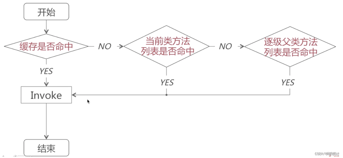
iOS消息发送流程
Objc的方法调用基于消息发送机制。即Objc中的方法调用,在底层实际都是通过调用objc_msgSend方法向对象消息发送消息来实现的。在iOS中, 实例对象的方法主要存储在类的方法列表中,类方法则是主要存储在原类中。 向对象发送消息,核心…...
【接口测试】常见HTTP面试题
目录 HTTP GET 和 POST 的区别 GET 和 POST 方法都是安全和幂等的吗 接口幂等实现方式 说说 post 请求的几种参数格式是什么样的? HTTP特性 HTTP(1.1) 的优点有哪些? HTTP(1.1) 的缺点有哪些&#x…...
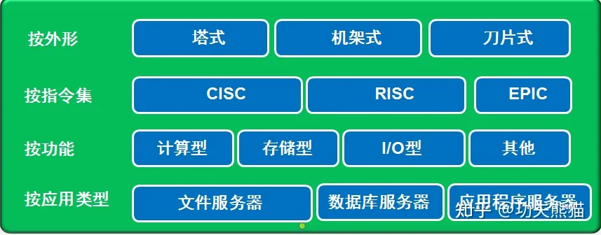
服务器硬件基础知识
1. 服务器分类 服务器分类 服务器的分类没有一个统一的标准。 从多个多个维度来看服务器的分类可以加深我们对各种服务器的认识。 N.B. CISC: complex instruction set computing 复杂指令集计算 RISC: reduced instruction set computer 精简指令集计算 EPIC: explicitly p…...
matlab实现层次聚类与k-均值聚类算法
1. 原理 1.层次聚类:通过计算两类数据点间的相似性,对所有数据点中最为相似的两个数据点进行组合,并反复迭代这一过程并生成聚类树 2.k-means聚类:在数据集中根据一定策略选择K个点作为每个簇的初始中心,然后将数据划…...

【机器学习】包裹式特征选择之递归特征消除法
🎈个人主页:豌豆射手^ 🎉欢迎 👍点赞✍评论⭐收藏 🤗收录专栏:机器学习 🤝希望本文对您有所裨益,如有不足之处,欢迎在评论区提出指正,让我们共同学习、交流进…...

【ArcGIS】重采样栅格像元匹配问题:不同空间分辨率栅格数据统一
重采样栅格像元匹配问题:不同空间分辨率栅格数据统一 原始数据数据1:GDP分布数据2.1:人口密度数据2.2:人口总数数据3:土地利用类型 数据处理操作1:将人口密度数据投影至GDP数据(栅格数据的投影变…...

Qt 简约又简单的加载动画 第七季 音量柱风格
今天和大家分享两个音量柱风格的加载动画,这次的加载动画的最大特点就是简单,只有几行代码. 效果如下: 一共三个文件,可以直接编译运行 //main.cpp #include "LoadingAnimWidget.h" #include <QApplication> #include <QGridLayout> int main(int argc…...

【JS】数值精度缺失问题解决方案
方法一: 保留字符串类型,传给后端 方法二: 如果涉及到计算,用以下方法 // 核心思想 在计算前,将数字乘以相同倍数,让他没有小数位,然后再进行计算,然后再除以相同的倍数࿰…...
c++基础知识补充4
单独使用词汇 using std::cout; 隐式类型转换型初始化:如A a1,,此时可以形象地理解为int i1;double ji;,此时1可以认为创建了一个值为1的临时对象,然后对目标对象进行赋值,当对象为多参数时,使用(1…...

leetcode230. 二叉搜索树中第K小的元素
lletcode 230. 二叉搜索树中第K小的元素,链接:https://leetcode.cn/problems/kth-smallest-element-in-a-bst 题目描述 给定一个二叉搜索树的根节点 root ,和一个整数 k ,请你设计一个算法查找其中第 k 个最小元素(从 …...

医学大数据|文献阅读|有关“肠癌+机器学习”的研究记录
目录 1.机器学习算法识别结直肠癌中的免疫相关lncRNA signature 2.基于机器学习的糖酵解相关分子分类揭示了结直肠癌癌症患者预后、TME和免疫疗法的差异,2区7 3.整合深度学习-病理组学、放射组学和免疫评分预测结直肠癌肺转移患者术后结局 4.最新7.4分纯生信&am…...
Linux信号【systemV】
目录 前言 正文: 1消息队列 1.1什么是消息队列? 1.2消息队列的数据结构 1.3消息队列的相关接口 1.3.1创建 1.3.2释放 1.3.3发送 1.3.4接收 1.4消息队列补充 2.信号量 2.1什么是信号量 2.2互斥相关概念 2.3信号量的数据结构 2.4…...

node.js最准确历史版本下载
先进入官网:Node.js https://nodejs.org/en 嫌其他博客多可以到/release下载:Node.js,在blog后面加/release https://nodejs.org/en/blog/release/ 点击next翻页,同样的道理...

UE5 C++ 单播 多播代理 动态多播代理
一. 代理机制,代理也叫做委托,其作用就是提供一种消息机制。 发送方 ,接收方 分别叫做 触发点和执行点。就是软件中的观察者模式的原理。 创建一个C Actor作为练习 二.单播代理 创建一个C Actor MyDeligateActor作为练习 在MyDeligateAc…...

前端学习、CSS
CSS可以嵌入到HTML中使用。 每个CSS语法包含两部分,选择器和应用的属性。 div用来声明针对页面上的哪些元素生效。 具体设置的属性以键值对形式表示,属性都在{}里,属性之间用;分割,键和值之间用:分割。 因为CSS的特殊命名风格…...
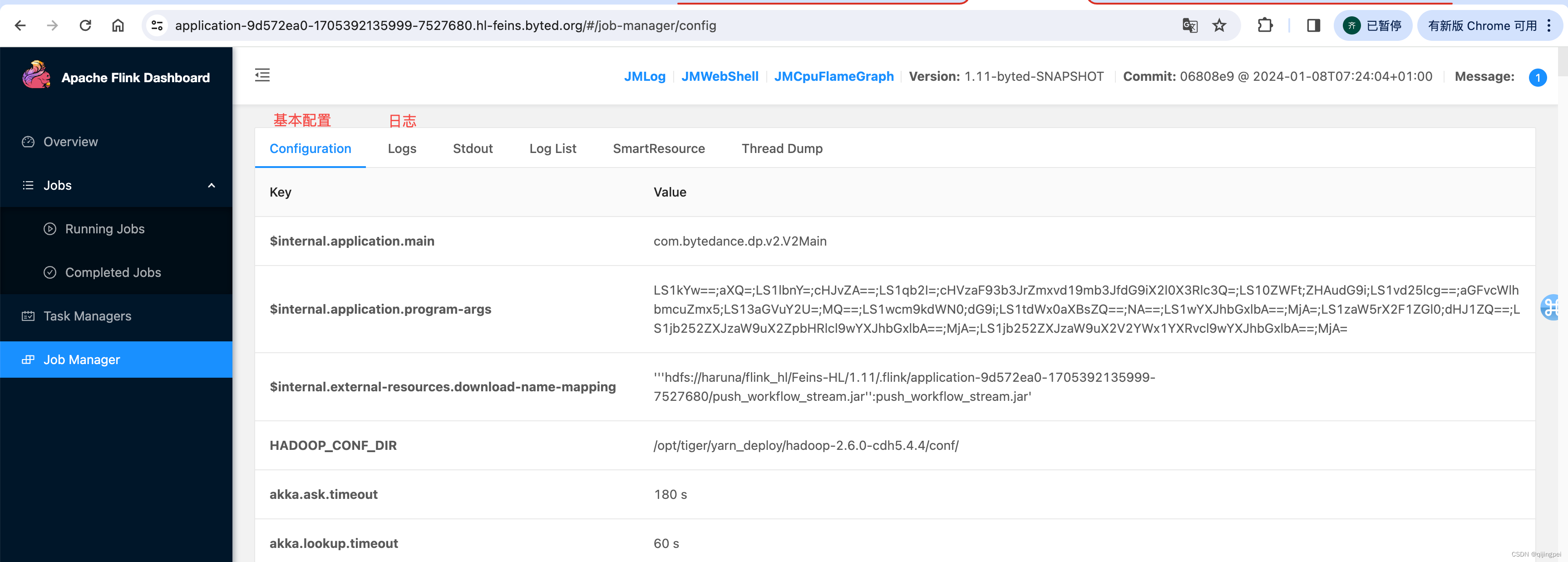
Flink基本原理 + WebUI说明 + 常见问题分析
Flink 概述 Flink 是一个用于进行大规模数据处理的开源框架,它提供了一个流式的数据处理 API,支持多种编程语言和运行时环境。Flink 的核心优点包括: 低延迟:Flink 可以在毫秒级的时间内处理数据,提供了低延迟的数据…...
)
3. 文档概述(Documentation Overview)
3. 文档概述(Documentation Overview) 本章节简要介绍一下Spring Boot参考文档。它包含本文档其它部分的链接。 本文档的最新版本可在 docs.spring.io/spring-boot/docs/current/reference/ 上获取。 3.1 第一步(First Steps) …...

【vue3 路由使用与讲解】vue-router : 简洁直观的全面介绍
# 核心内容介绍 路由跳转有两种方式: 声明式导航:<router-link :to"...">编程式导航:router.push(...) 或 router.replace(...) ;两者的规则完全一致。 push(to: RouteLocationRaw): Promise<NavigationFailur…...

本地Cookie导出工具:解决Web开发中的认证数据管理难题
本地Cookie导出工具:解决Web开发中的认证数据管理难题 【免费下载链接】Get-cookies.txt-LOCALLY Get cookies.txt, NEVER send information outside. 项目地址: https://gitcode.com/gh_mirrors/ge/Get-cookies.txt-LOCALLY 在Web开发和数据采集领域&#x…...

Happy Island Designer终极指南:从零开始打造梦想岛屿的完整教程
Happy Island Designer终极指南:从零开始打造梦想岛屿的完整教程 【免费下载链接】HappyIslandDesigner "Happy Island Designer (Alpha)",是一个在线工具,它允许用户设计和定制自己的岛屿。这个工具是受游戏《动物森友会》(Animal…...

CC工具箱实战:SHP转TXT通用版,从数据到自定义描述的完整流程
1. 为什么需要SHP转TXT工具? 在日常的GIS数据处理工作中,我们经常会遇到需要将SHP格式的地块数据转换为特定格式的TXT文件的需求。比如在土地调查项目中,上级部门可能要求提交包含地块坐标和属性的文本文件;在数据上报时ÿ…...

如何用Cyberbrain在5分钟内调试复杂的Python循环问题
如何用Cyberbrain在5分钟内调试复杂的Python循环问题 【免费下载链接】Cyberbrain Python debugging, redefined. 项目地址: https://gitcode.com/gh_mirrors/cy/Cyberbrain 调试Python循环问题常常让开发者头疼,尤其是面对多层嵌套或复杂逻辑时,…...

从PCI到PCIe:一次Read请求的‘分家’之旅,以及超时机制为何成了‘必要之恶’
从PCI到PCIe:一次Read请求的‘分家’之旅,以及超时机制为何成了‘必要之恶’ 在计算机体系结构的演进长河中,总线协议的设计始终面临着效率与可靠性的永恒博弈。想象一下,当CPU需要从外设读取数据时,如果必须像排队买奶…...

LabVIEW网络通讯:TCP连接三菱PLC FX3U ENET-ADP的MC协议网络通讯与程序开发
LabVIEW网络网口TCP通讯三菱PLC FX3U ENET-ADP,MC协议网络通讯FX3U网络通讯。 官方MC协议,报文读取,安全稳定。 程序代开发,代写程序。 通讯配置,辅助测试。 FX3U无程序网络通讯实现。 常用功能一网打尽。 1.命令帧读写…...

智能Agent核心组件:基于BERT文本分割的任务指令分解模块
智能Agent核心组件:基于BERT文本分割的任务指令分解模块 你有没有遇到过这种情况?对着一个智能助手说:“帮我查一下明天北京的天气,然后告诉我穿什么衣服合适,再推荐几个室内的活动。” 然后,它要么只回答…...
)
Axure疑难杂症:利用中继器制作三级下拉菜单(逻辑判断进阶)
亲爱的小伙伴,在您浏览之前,烦请关注一下,在此深表感谢! Axure产品经理精品视频课已登录CSDN可点击学习https://edu.csdn.net/course/detail/40420 课程主题:三级下拉菜单 主要内容:条件筛选时的逻辑判断思维,中继器使用 应用场景:复合条件下的下拉列表制作 案例展…...

【算法优化】基于网格划分的高效DBSCAN改进策略
1. 为什么需要优化DBSCAN算法? 第一次接触DBSCAN算法时,我被它的聚类能力惊艳到了——不需要预先指定簇数量,还能识别任意形状的簇。但当我用真实数据集测试时,电脑直接卡死,这才发现传统DBSCAN的O(n)时间复杂度有多可…...
FDE会被AI完全替代吗?)
Palantir:两个不确定的问题(2)FDE会被AI完全替代吗?
从上一篇的分析可以得知,Palantir的整套系统,就是一个有机的企业级数字孪生体: 本体Ontology灵魂/主宰 它定义世界“是什么、有什么、彼此关系如何”,是客观现实与人类主观认识的统一,是整个系统的 “道”。 AIP心与…...