从零开始学习Diffusion Models: Sharon Zhou
How Diffusion Models Work
本文是 https://www.deeplearning.ai/short-courses/how-diffusion-models-work/ 这门课程的学习笔记。
文章目录
- How Diffusion Models Work
- What you’ll learn in this course
- [1] Intuition
- [2] Sampling
- Setting Things Up
- Sampling
- Demonstrate incorrectly sample without adding the 'extra noise'
- Acknowledgments
- [3] Neural Network
- [4] Training
- Setting Things Up
- Training
- Sampling
- View Epoch 0
- View Epoch 4
- View Epoch 8
- View Epoch 31
- [5] Controlling
- Setting Things Up
- Context
- Sampling with context
- [6] Speeding up
- Setting Things Up
- Fast Sampling
- Compare DDPM, DDIM speed
- 后记
How Diffusion Models Work:Sharon Zhou
What you’ll learn in this course
In How Diffusion Models Work, you will gain a deep familiarity with the diffusion process and the models which carry it out. More than simply pulling in a pre-built model or using an API, this course will teach you to build a diffusion model from scratch.
In this course you will:
- Explore the cutting-edge world of diffusion-based generative AI and create your own diffusion model from scratch.
- Gain deep familiarity with the diffusion process and the models driving it, going beyond pre-built models and APIs.
- Acquire practical coding skills by working through labs on sampling, training diffusion models, building neural networks for noise prediction, and adding context for personalized image generation.
At the end of the course, you will have a model that can serve as a starting point for your own exploration of diffusion models for your applications.
This one-hour course, taught by Sharon Zhou will expand your generative AI capabilities to include building, training, and optimizing diffusion models.
Hands-on examples make the concepts easy to understand and build upon. Built-in Jupyter notebooks allow you to seamlessly experiment with the code and labs presented in the course.
[1] Intuition
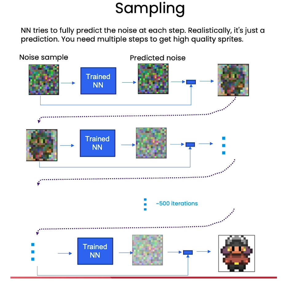
[2] Sampling
from typing import Dict, Tuple
from tqdm import tqdm
import torch
import torch.nn as nn
import torch.nn.functional as F
from torch.utils.data import DataLoader
from torchvision import models, transforms
from torchvision.utils import save_image, make_grid
import matplotlib.pyplot as plt
from matplotlib.animation import FuncAnimation, PillowWriter
import numpy as np
from IPython.display import HTML
from diffusion_utilities import *
Setting Things Up
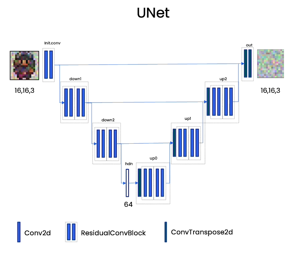
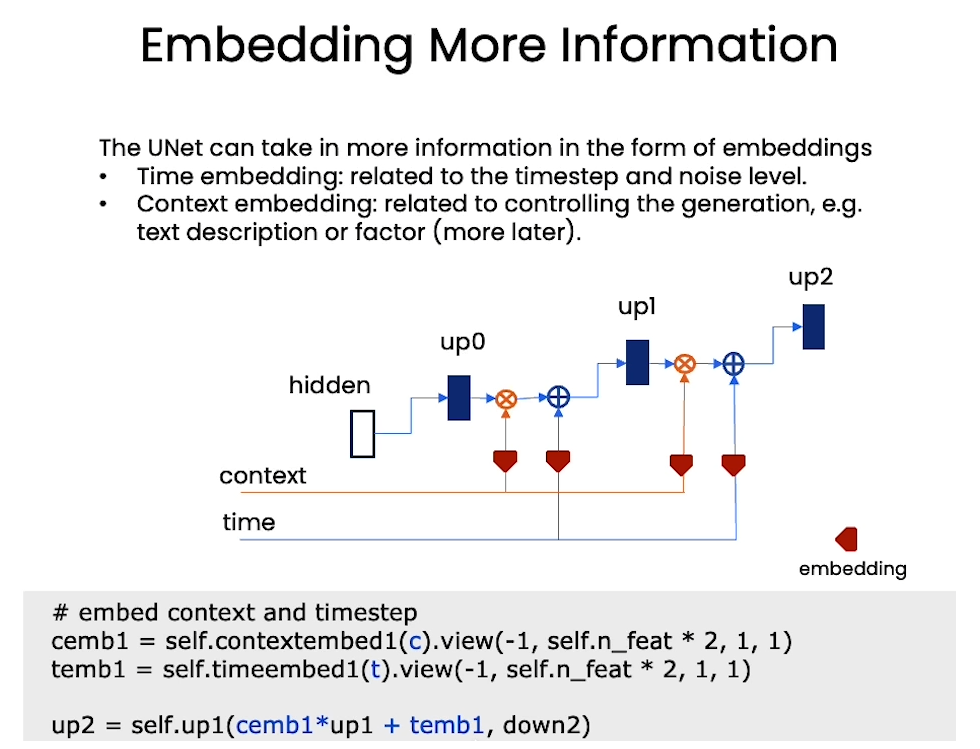
class ContextUnet(nn.Module):def __init__(self, in_channels, n_feat=256, n_cfeat=10, height=28): # cfeat - context featuressuper(ContextUnet, self).__init__()# number of input channels, number of intermediate feature maps and number of classesself.in_channels = in_channelsself.n_feat = n_featself.n_cfeat = n_cfeatself.h = height #assume h == w. must be divisible by 4, so 28,24,20,16...# Initialize the initial convolutional layerself.init_conv = ResidualConvBlock(in_channels, n_feat, is_res=True)# Initialize the down-sampling path of the U-Net with two levelsself.down1 = UnetDown(n_feat, n_feat) # down1 #[10, 256, 8, 8]self.down2 = UnetDown(n_feat, 2 * n_feat) # down2 #[10, 256, 4, 4]# original: self.to_vec = nn.Sequential(nn.AvgPool2d(7), nn.GELU())self.to_vec = nn.Sequential(nn.AvgPool2d((4)), nn.GELU())# Embed the timestep and context labels with a one-layer fully connected neural networkself.timeembed1 = EmbedFC(1, 2*n_feat)self.timeembed2 = EmbedFC(1, 1*n_feat)self.contextembed1 = EmbedFC(n_cfeat, 2*n_feat)self.contextembed2 = EmbedFC(n_cfeat, 1*n_feat)# Initialize the up-sampling path of the U-Net with three levelsself.up0 = nn.Sequential(nn.ConvTranspose2d(2 * n_feat, 2 * n_feat, self.h//4, self.h//4), # up-sample nn.GroupNorm(8, 2 * n_feat), # normalize nn.ReLU(),)self.up1 = UnetUp(4 * n_feat, n_feat)self.up2 = UnetUp(2 * n_feat, n_feat)# Initialize the final convolutional layers to map to the same number of channels as the input imageself.out = nn.Sequential(nn.Conv2d(2 * n_feat, n_feat, 3, 1, 1), # reduce number of feature maps #in_channels, out_channels, kernel_size, stride=1, padding=0nn.GroupNorm(8, n_feat), # normalizenn.ReLU(),nn.Conv2d(n_feat, self.in_channels, 3, 1, 1), # map to same number of channels as input)def forward(self, x, t, c=None):"""x : (batch, n_feat, h, w) : input imaget : (batch, n_cfeat) : time stepc : (batch, n_classes) : context label"""# x is the input image, c is the context label, t is the timestep, context_mask says which samples to block the context on# pass the input image through the initial convolutional layerx = self.init_conv(x)# pass the result through the down-sampling pathdown1 = self.down1(x) #[10, 256, 8, 8]down2 = self.down2(down1) #[10, 256, 4, 4]# convert the feature maps to a vector and apply an activationhiddenvec = self.to_vec(down2) # hiddenvec 的维度应该为 [10, 256, 1, 1]# AvgPool2d((4)) 操作:#这个操作是一个平均池化(Average Pooling)层,将特征图的每个 4x4 区域的值取平均。由于特征图 down2 的维度为 [10, 256, 4, 4],经过 #AvgPool2d((4)) 操作后,每个特征图将被降采样为一个单一的值。因此,输出的形状将变为 [10, 256, 1, 1]。# mask out context if context_mask == 1if c is None:c = torch.zeros(x.shape[0], self.n_cfeat).to(x)# embed context and timestepcemb1 = self.contextembed1(c).view(-1, self.n_feat * 2, 1, 1) # (batch, 2*n_feat, 1,1)temb1 = self.timeembed1(t).view(-1, self.n_feat * 2, 1, 1)cemb2 = self.contextembed2(c).view(-1, self.n_feat, 1, 1)temb2 = self.timeembed2(t).view(-1, self.n_feat, 1, 1)print(f"uunet forward: cemb1 {cemb1.shape}. temb1 {temb1.shape}, cemb2 {cemb2.shape}. temb2 {temb2.shape}")# uunet forward: cemb1 torch.Size([32, 128, 1, 1]). # temb1 torch.Size([1, 128, 1, 1]), # cemb2 torch.Size([32, 64, 1, 1]). # temb2 torch.Size([1, 64, 1, 1])up1 = self.up0(hiddenvec) # hiddenvec 的维度应该为 [10, 256, 1, 1]up2 = self.up1(cemb1*up1 + temb1, down2) # add and multiply embeddingsup3 = self.up2(cemb2*up2 + temb2, down1)out = self.out(torch.cat((up3, x), 1))return out根据代码和已知信息,我们可以推断 up1, up2, up3 和 out 的输出维度如下:
-
对于
up1:- 输入是
hiddenvec,其形状为(batch_size, n_feat, 1, 1)。 up0中的转置卷积操作会将输入进行上采样,输出的形状将与down2的特征图相同,即(batch_size, 2*n_feat, h/4, w/4)。
- 输入是
-
对于
up2:- 输入是
cemb1 * up1 + temb1,其中cemb1的形状为(batch_size, 2*n_feat, 1, 1),up1的形状为(batch_size, 2*n_feat, h/4, w/4),temb1的形状为(batch_size, 2*n_feat, 1, 1)。 - 这些张量相加后,其形状应该仍然是
(batch_size, 2*n_feat, h/4, w/4)。 up1中的上采样操作将输出的特征图大小恢复为原来的一半,因此,up2的输出形状将是(batch_size, n_feat, h/2, w/2)。
- 输入是
-
对于
up3:- 输入是
cemb2 * up2 + temb2,其中cemb2的形状为(batch_size, n_feat, 1, 1),up2的形状为(batch_size, n_feat, h/2, w/2),temb2的形状为(batch_size, n_feat, 1, 1)。 - 这些张量相加后,其形状应该仍然是
(batch_size, n_feat, h/2, w/2)。 up2中的上采样操作将输出的特征图大小恢复为原来的一半,因此,up3的输出形状将是(batch_size, n_feat, h, w)。
- 输入是
-
对于
out:- 输入是将
up3和原始输入x拼接在一起,up3的形状为(batch_size, n_feat, h, w),x的形状为(batch_size, in_channels, h, w)。 - 因此,拼接后输入通道的数量为
n_feat + in_channels。 out的输出形状应该是(batch_size, in_channels, h, w),与原始输入的图像大小相同。
- 输入是将
综上所述,up1 的输出形状为 (batch_size, 2*n_feat, h/4, w/4),up2 的输出形状为 (batch_size, n_feat, h/2, w/2),up3 的输出形状为 (batch_size, n_feat, h, w),而 out 的输出形状应该是 (batch_size, in_channels, h, w)。
有用的函数:diffusion_utilities.py文件如下
import torch
import torch.nn as nn
import numpy as np
from torchvision.utils import save_image, make_grid
import matplotlib.pyplot as plt
from matplotlib.animation import FuncAnimation, PillowWriter
import os
import torchvision.transforms as transforms
from torch.utils.data import Dataset
from PIL import Imageclass ResidualConvBlock(nn.Module):def __init__(self, in_channels: int, out_channels: int, is_res: bool = False) -> None:super().__init__()# Check if input and output channels are the same for the residual connectionself.same_channels = in_channels == out_channels# Flag for whether or not to use residual connectionself.is_res = is_res# First convolutional layerself.conv1 = nn.Sequential(nn.Conv2d(in_channels, out_channels, 3, 1, 1),   # 3x3 kernel with stride 1 and padding 1nn.BatchNorm2d(out_channels),   # Batch normalizationnn.GELU(),   # GELU activation function)# Second convolutional layerself.conv2 = nn.Sequential(nn.Conv2d(out_channels, out_channels, 3, 1, 1),   # 3x3 kernel with stride 1 and padding 1nn.BatchNorm2d(out_channels),   # Batch normalizationnn.GELU(),   # GELU activation function)def forward(self, x: torch.Tensor) -> torch.Tensor:# If using residual connectionif self.is_res:# Apply first convolutional layerx1 = self.conv1(x)# Apply second convolutional layerx2 = self.conv2(x1)# If input and output channels are the same, add residual connection directlyif self.same_channels:out = x + x2else:# If not, apply a 1x1 convolutional layer to match dimensions before adding residual connectionshortcut = nn.Conv2d(x.shape[1], x2.shape[1], kernel_size=1, stride=1, padding=0).to(x.device)out = shortcut(x) + x2#print(f"resconv forward: x {x.shape}, x1 {x1.shape}, x2 {x2.shape}, out {out.shape}")# Normalize output tensorreturn out / 1.414# If not using residual connection, return output of second convolutional layerelse:x1 = self.conv1(x)x2 = self.conv2(x1)return x2# Method to get the number of output channels for this blockdef get_out_channels(self):return self.conv2[0].out_channels# Method to set the number of output channels for this blockdef set_out_channels(self, out_channels):self.conv1[0].out_channels = out_channelsself.conv2[0].in_channels = out_channelsself.conv2[0].out_channels = out_channelsclass UnetUp(nn.Module):def __init__(self, in_channels, out_channels):super(UnetUp, self).__init__()# Create a list of layers for the upsampling block# The block consists of a ConvTranspose2d layer for upsampling, followed by two ResidualConvBlock layerslayers = [nn.ConvTranspose2d(in_channels, out_channels, 2, 2),ResidualConvBlock(out_channels, out_channels),ResidualConvBlock(out_channels, out_channels),]# Use the layers to create a sequential modelself.model = nn.Sequential(*layers)def forward(self, x, skip):# Concatenate the input tensor x with the skip connection tensor along the channel dimensionx = torch.cat((x, skip), 1)# Pass the concatenated tensor through the sequential model and return the outputx = self.model(x)return xclass UnetDown(nn.Module):def __init__(self, in_channels, out_channels):super(UnetDown, self).__init__()# Create a list of layers for the downsampling block# Each block consists of two ResidualConvBlock layers, followed by a MaxPool2d layer for downsamplinglayers = [ResidualConvBlock(in_channels, out_channels), ResidualConvBlock(out_channels, out_channels), nn.MaxPool2d(2)]# Use the layers to create a sequential modelself.model = nn.Sequential(*layers)def forward(self, x):# Pass the input through the sequential model and return the outputreturn self.model(x)class EmbedFC(nn.Module):def __init__(self, input_dim, emb_dim):super(EmbedFC, self).__init__()'''This class defines a generic one layer feed-forward neural network for embedding input data ofdimensionality input_dim to an embedding space of dimensionality emb_dim.'''self.input_dim = input_dim# define the layers for the networklayers = [nn.Linear(input_dim, emb_dim),nn.GELU(),nn.Linear(emb_dim, emb_dim),]# create a PyTorch sequential model consisting of the defined layersself.model = nn.Sequential(*layers)def forward(self, x):# flatten the input tensorx = x.view(-1, self.input_dim)# apply the model layers to the flattened tensorreturn self.model(x)
测试ResidualConvBlock类
import torch
import torch.nn as nn# 创建一个ResidualConvBlock实例
residual_block = ResidualConvBlock(in_channels=3, out_channels=3, is_res=True)# 创建一个测试输入张量
x = torch.randn(1, 3, 32, 32)  # 假设输入张量的形状为(batch_size, in_channels, height, width)# 使用ResidualConvBlock进行前向传播
output = residual_block(x)print(output.shape)
这个例子假设输入张量的形状是 (1, 3, 32, 32),即一个 3 通道、高度和宽度均为 32 像素的图像。在这个例子中,我们使用了残差连接,并且输入和输出通道数量相同。我们预期输出应该与输入张量的形状相同 (1, 3, 32, 32)。
# hyperparameters# diffusion hyperparameters
timesteps = 500
beta1 = 1e-4
beta2 = 0.02# network hyperparameters
device = torch.device("cuda:0" if torch.cuda.is_available() else torch.device('cpu'))
n_feat = 64 # 64 hidden dimension feature
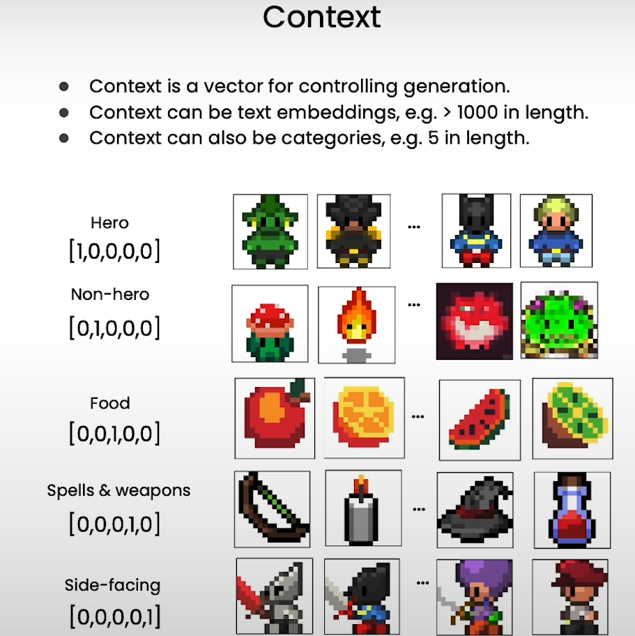
n_cfeat = 5 # context vector is of size 5
height = 16 # 16x16 image
save_dir = './weights/'
# construct DDPM noise schedule
b_t = (beta2 - beta1) * torch.linspace(0, 1, timesteps + 1, device=device) + beta1
a_t = 1 - b_t
ab_t = torch.cumsum(a_t.log(), dim=0).exp()
ab_t[0] = 1
# construct model
nn_model = ContextUnet(in_channels=3, n_feat=n_feat, n_cfeat=n_cfeat, height=height).to(device)
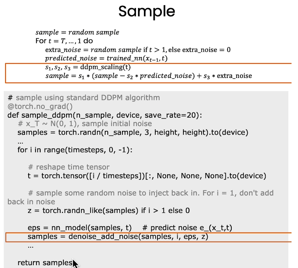
Sampling
# helper function; removes the predicted noise (but adds some noise back in to avoid collapse)
def denoise_add_noise(x, t, pred_noise, z=None):if z is None:z = torch.randn_like(x)noise = b_t.sqrt()[t] * zmean = (x - pred_noise * ((1 - a_t[t]) / (1 - ab_t[t]).sqrt())) / a_t[t].sqrt()return mean + noise
# load in model weights and set to eval mode
nn_model.load_state_dict(torch.load(f"{save_dir}/model_trained.pth", map_location=device))
nn_model.eval()
print("Loaded in Model")
# sample using standard algorithm
@torch.no_grad()
def sample_ddpm(n_sample, save_rate=20):# x_T ~ N(0, 1), sample initial noisesamples = torch.randn(n_sample, 3, height, height).to(device)  # array to keep track of generated steps for plottingintermediate = [] for i in range(timesteps, 0, -1):print(f'sampling timestep {i:3d}', end='\r')# reshape time tensort = torch.tensor([i / timesteps])[:, None, None, None].to(device)# sample some random noise to inject back in. For i = 1, don't add back in noisez = torch.randn_like(samples) if i > 1 else 0eps = nn_model(samples, t)    # predict noise e_(x_t,t)samples = denoise_add_noise(samples, i, eps, z)if i % save_rate ==0 or i==timesteps or i<8:intermediate.append(samples.detach().cpu().numpy())intermediate = np.stack(intermediate)return samples, intermediate
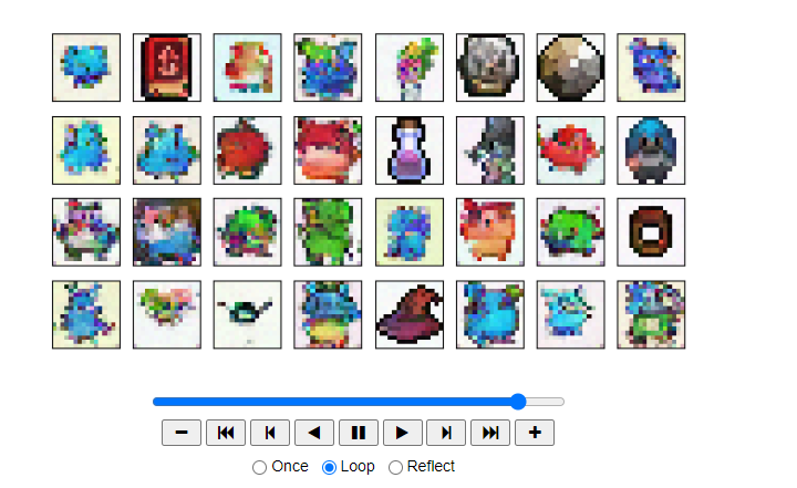
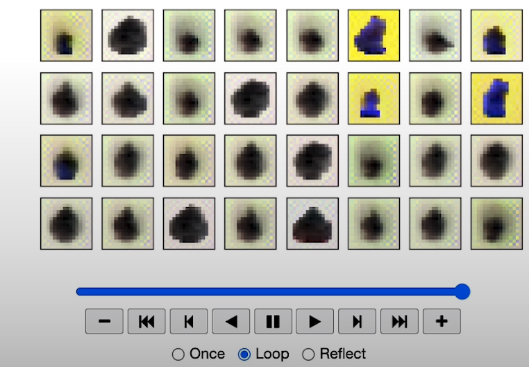
# visualize samples
plt.clf()
samples, intermediate_ddpm = sample_ddpm(32)
animation_ddpm = plot_sample(intermediate_ddpm,32,4,save_dir, "ani_run", None, save=False)
HTML(animation_ddpm.to_jshtml())
Output
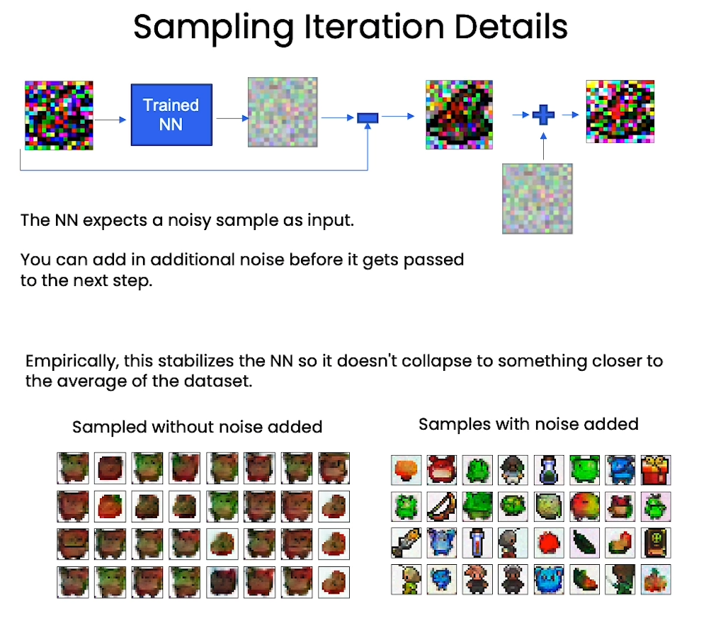
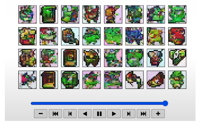
Demonstrate incorrectly sample without adding the ‘extra noise’
# incorrectly sample without adding in noise
@torch.no_grad()
def sample_ddpm_incorrect(n_sample):# x_T ~ N(0, 1), sample initial noisesamples = torch.randn(n_sample, 3, height, height).to(device)  # array to keep track of generated steps for plottingintermediate = [] for i in range(timesteps, 0, -1):print(f'sampling timestep {i:3d}', end='\r')# reshape time tensor# [:, None, None, None] 是一种广播操作,用于在 PyTorch 中扩展张量的维度。# 这段代码的作用是创建一个时间张量 t,该张量的形状为 (1, 1, 1, 1)t = torch.tensor([i / timesteps])[:, None, None, None].to(device)# don't add back in noisez = 0eps = nn_model(samples, t)    # predict noise e_(x_t,t)samples = denoise_add_noise(samples, i, eps, z)if i%20==0 or i==timesteps or i<8:intermediate.append(samples.detach().cpu().numpy())intermediate = np.stack(intermediate)return samples, intermediate
# visualize samples
plt.clf()
samples, intermediate = sample_ddpm_incorrect(32)
animation = plot_sample(intermediate,32,4,save_dir, "ani_run", None, save=False)
HTML(animation.to_jshtml())
Output
Acknowledgments
Sprites by ElvGames, FrootsnVeggies and kyrise
This code is modified from, https://github.com/cloneofsimo/minDiffusion
Diffusion model is based on Denoising Diffusion Probabilistic Models and Denoising Diffusion Implicit Models
[3] Neural Network
[4] Training
from typing import Dict, Tuple
from tqdm import tqdm
import torch
import torch.nn as nn
import torch.nn.functional as F
from torch.utils.data import DataLoader
from torchvision import models, transforms
from torchvision.utils import save_image, make_grid
import matplotlib.pyplot as plt
from matplotlib.animation import FuncAnimation, PillowWriter
import numpy as np
from IPython.display import HTML
from diffusion_utilities import *
Setting Things Up
class ContextUnet(nn.Module):def __init__(self, in_channels, n_feat=256, n_cfeat=10, height=28): # cfeat - context featuressuper(ContextUnet, self).__init__()# number of input channels, number of intermediate feature maps and number of classesself.in_channels = in_channelsself.n_feat = n_featself.n_cfeat = n_cfeatself.h = height #assume h == w. must be divisible by 4, so 28,24,20,16...# Initialize the initial convolutional layerself.init_conv = ResidualConvBlock(in_channels, n_feat, is_res=True)# Initialize the down-sampling path of the U-Net with two levelsself.down1 = UnetDown(n_feat, n_feat) # down1 #[10, 256, 8, 8]self.down2 = UnetDown(n_feat, 2 * n_feat) # down2 #[10, 256, 4, 4]# original: self.to_vec = nn.Sequential(nn.AvgPool2d(7), nn.GELU())self.to_vec = nn.Sequential(nn.AvgPool2d((4)), nn.GELU())# Embed the timestep and context labels with a one-layer fully connected neural networkself.timeembed1 = EmbedFC(1, 2*n_feat)self.timeembed2 = EmbedFC(1, 1*n_feat)self.contextembed1 = EmbedFC(n_cfeat, 2*n_feat)self.contextembed2 = EmbedFC(n_cfeat, 1*n_feat)# Initialize the up-sampling path of the U-Net with three levelsself.up0 = nn.Sequential(nn.ConvTranspose2d(2 * n_feat, 2 * n_feat, self.h//4, self.h//4), # up-sample nn.GroupNorm(8, 2 * n_feat), # normalize nn.ReLU(),)self.up1 = UnetUp(4 * n_feat, n_feat)self.up2 = UnetUp(2 * n_feat, n_feat)# Initialize the final convolutional layers to map to the same number of channels as the input imageself.out = nn.Sequential(nn.Conv2d(2 * n_feat, n_feat, 3, 1, 1), # reduce number of feature maps #in_channels, out_channels, kernel_size, stride=1, padding=0nn.GroupNorm(8, n_feat), # normalizenn.ReLU(),nn.Conv2d(n_feat, self.in_channels, 3, 1, 1), # map to same number of channels as input)def forward(self, x, t, c=None):"""x : (batch, n_feat, h, w) : input imaget : (batch, n_cfeat) : time stepc : (batch, n_classes) : context label"""# x is the input image, c is the context label, t is the timestep, context_mask says which samples to block the context on# pass the input image through the initial convolutional layerx = self.init_conv(x)# pass the result through the down-sampling pathdown1 = self.down1(x) #[10, 256, 8, 8]down2 = self.down2(down1) #[10, 256, 4, 4]# convert the feature maps to a vector and apply an activationhiddenvec = self.to_vec(down2)# mask out context if context_mask == 1if c is None:c = torch.zeros(x.shape[0], self.n_cfeat).to(x)# embed context and timestepcemb1 = self.contextembed1(c).view(-1, self.n_feat * 2, 1, 1) # (batch, 2*n_feat, 1,1)temb1 = self.timeembed1(t).view(-1, self.n_feat * 2, 1, 1)cemb2 = self.contextembed2(c).view(-1, self.n_feat, 1, 1)temb2 = self.timeembed2(t).view(-1, self.n_feat, 1, 1)#print(f"uunet forward: cemb1 {cemb1.shape}. temb1 {temb1.shape}, cemb2 {cemb2.shape}. temb2 {temb2.shape}")up1 = self.up0(hiddenvec)up2 = self.up1(cemb1*up1 + temb1, down2) # add and multiply embeddingsup3 = self.up2(cemb2*up2 + temb2, down1)out = self.out(torch.cat((up3, x), 1))return out# hyperparameters# diffusion hyperparameters
timesteps = 500
beta1 = 1e-4
beta2 = 0.02# network hyperparameters
device = torch.device("cuda:0" if torch.cuda.is_available() else torch.device('cpu'))
n_feat = 64 # 64 hidden dimension feature
n_cfeat = 5 # context vector is of size 5
height = 16 # 16x16 image
save_dir = './weights/'# training hyperparameters
batch_size = 100
n_epoch = 32
lrate=1e-3
# construct DDPM noise schedule
b_t = (beta2 - beta1) * torch.linspace(0, 1, timesteps + 1, device=device) + beta1
a_t = 1 - b_t
ab_t = torch.cumsum(a_t.log(), dim=0).exp()
ab_t[0] = 1# construct model
nn_model = ContextUnet(in_channels=3, n_feat=n_feat, n_cfeat=n_cfeat, height=height).to(device)
Training
# load dataset and construct optimizer
dataset = CustomDataset("./sprites_1788_16x16.npy", "./sprite_labels_nc_1788_16x16.npy", transform, null_context=False)
dataloader = DataLoader(dataset, batch_size=batch_size, shuffle=True, num_workers=1)
optim = torch.optim.Adam(nn_model.parameters(), lr=lrate)
Output
sprite shape: (89400, 16, 16, 3)
labels shape: (89400, 5)
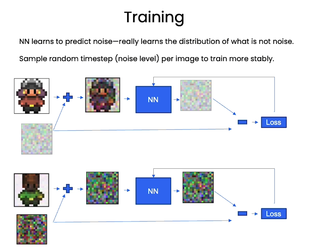
# helper function: perturbs an image to a specified noise level
def perturb_input(x, t, noise):return ab_t.sqrt()[t, None, None, None] * x + (1 - ab_t[t, None, None, None]) * noise
This code will take hours to run on a CPU. We recommend you skip this step here and check the intermediate results below.
If you decide to try it, you could download to your own machine. Be sure to change the cell type.
Note, the CPU run time in the course is limited so you will not be able to fully train the network using the class platform.
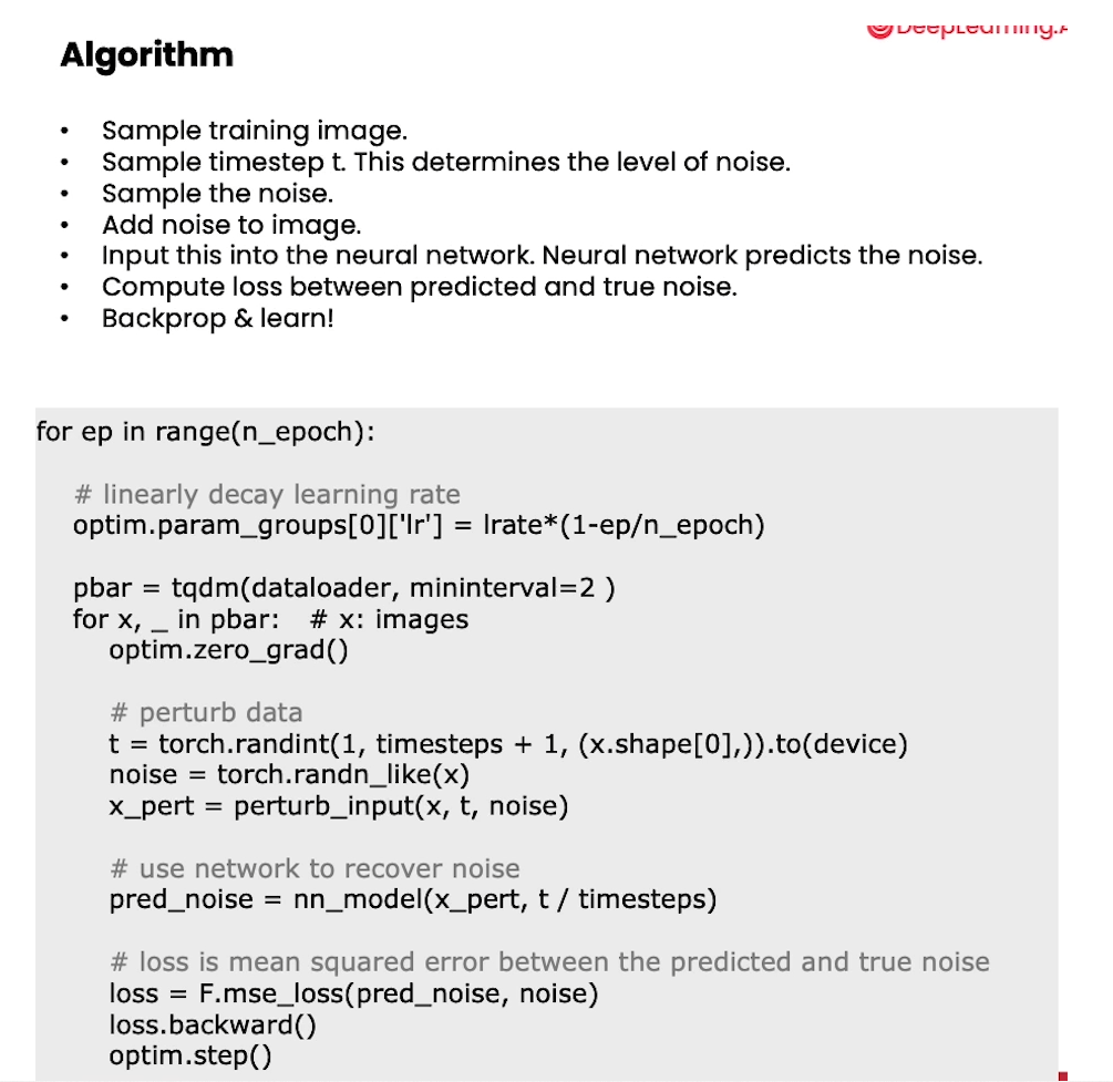
# training without context code# set into train mode
nn_model.train()for ep in range(n_epoch):print(f'epoch {ep}')# linearly decay learning rateoptim.param_groups[0]['lr'] = lrate*(1-ep/n_epoch)pbar = tqdm(dataloader, mininterval=2 )for x, _ in pbar:   # x: imagesoptim.zero_grad()x = x.to(device)# perturb datanoise = torch.randn_like(x)t = torch.randint(1, timesteps + 1, (x.shape[0],)).to(device) x_pert = perturb_input(x, t, noise)# use network to recover noisepred_noise = nn_model(x_pert, t / timesteps)# loss is mean squared error between the predicted and true noiseloss = F.mse_loss(pred_noise, noise)loss.backward()optim.step()# save model periodicallyif ep%4==0 or ep == int(n_epoch-1):if not os.path.exists(save_dir):os.mkdir(save_dir)torch.save(nn_model.state_dict(), save_dir + f"model_{ep}.pth")print('saved model at ' + save_dir + f"model_{ep}.pth")
Sampling
# helper function; removes the predicted noise (but adds some noise back in to avoid collapse)
def denoise_add_noise(x, t, pred_noise, z=None):if z is None:z = torch.randn_like(x)noise = b_t.sqrt()[t] * zmean = (x - pred_noise * ((1 - a_t[t]) / (1 - ab_t[t]).sqrt())) / a_t[t].sqrt()return mean + noise
# sample using standard algorithm
@torch.no_grad()
def sample_ddpm(n_sample, save_rate=20):# x_T ~ N(0, 1), sample initial noisesamples = torch.randn(n_sample, 3, height, height).to(device)  # array to keep track of generated steps for plottingintermediate = [] for i in range(timesteps, 0, -1):print(f'sampling timestep {i:3d}', end='\r')# reshape time tensort = torch.tensor([i / timesteps])[:, None, None, None].to(device)# sample some random noise to inject back in. For i = 1, don't add back in noisez = torch.randn_like(samples) if i > 1 else 0eps = nn_model(samples, t)    # predict noise e_(x_t,t)samples = denoise_add_noise(samples, i, eps, z)if i % save_rate ==0 or i==timesteps or i<8:intermediate.append(samples.detach().cpu().numpy())intermediate = np.stack(intermediate)return samples, intermediate
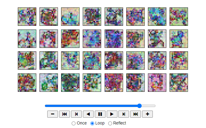
View Epoch 0
# load in model weights and set to eval mode
nn_model.load_state_dict(torch.load(f"{save_dir}/model_0.pth", map_location=device))
nn_model.eval()
print("Loaded in Model")
# visualize samples
plt.clf()
samples, intermediate_ddpm = sample_ddpm(32)
animation_ddpm = plot_sample(intermediate_ddpm,32,4,save_dir, "ani_run", None, save=False)
HTML(animation_ddpm.to_jshtml())
Output
View Epoch 4
# load in model weights and set to eval mode
nn_model.load_state_dict(torch.load(f"{save_dir}/model_4.pth", map_location=device))
nn_model.eval()
print("Loaded in Model")# visualize samples
plt.clf()
samples, intermediate_ddpm = sample_ddpm(32)
animation_ddpm = plot_sample(intermediate_ddpm,32,4,save_dir, "ani_run", None, save=False)
HTML(animation_ddpm.to_jshtml())
Output
View Epoch 8
# load in model weights and set to eval mode
nn_model.load_state_dict(torch.load(f"{save_dir}/model_8.pth", map_location=device))
nn_model.eval()
print("Loaded in Model")# visualize samples
plt.clf()
samples, intermediate_ddpm = sample_ddpm(32)
animation_ddpm = plot_sample(intermediate_ddpm,32,4,save_dir, "ani_run", None, save=False)
HTML(animation_ddpm.to_jshtml())
Output
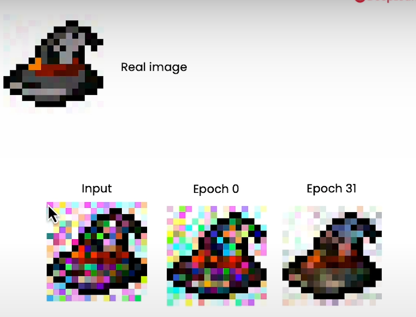
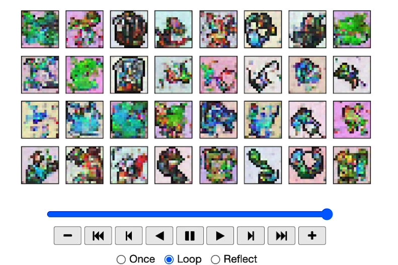
View Epoch 31
# load in model weights and set to eval mode
nn_model.load_state_dict(torch.load(f"{save_dir}/model_31.pth", map_location=device))
nn_model.eval()
print("Loaded in Model")# visualize samples
plt.clf()
samples, intermediate_ddpm = sample_ddpm(32)
animation_ddpm = plot_sample(intermediate_ddpm,32,4,save_dir, "ani_run", None, save=False)
HTML(animation_ddpm.to_jshtml())
Output
[5] Controlling
from typing import Dict, Tuple
from tqdm import tqdm
import torch
import torch.nn as nn
import torch.nn.functional as F
from torch.utils.data import DataLoader
from torchvision import models, transforms
from torchvision.utils import save_image, make_grid
import matplotlib.pyplot as plt
from matplotlib.animation import FuncAnimation, PillowWriter
import numpy as np
from IPython.display import HTML
from diffusion_utilities import *
Setting Things Up
class ContextUnet(nn.Module):def __init__(self, in_channels, n_feat=256, n_cfeat=10, height=28): # cfeat - context featuressuper(ContextUnet, self).__init__()# number of input channels, number of intermediate feature maps and number of classesself.in_channels = in_channelsself.n_feat = n_featself.n_cfeat = n_cfeatself.h = height #assume h == w. must be divisible by 4, so 28,24,20,16...# Initialize the initial convolutional layerself.init_conv = ResidualConvBlock(in_channels, n_feat, is_res=True)# Initialize the down-sampling path of the U-Net with two levelsself.down1 = UnetDown(n_feat, n_feat) # down1 #[10, 256, 8, 8]self.down2 = UnetDown(n_feat, 2 * n_feat) # down2 #[10, 256, 4, 4]# original: self.to_vec = nn.Sequential(nn.AvgPool2d(7), nn.GELU())self.to_vec = nn.Sequential(nn.AvgPool2d((4)), nn.GELU())# Embed the timestep and context labels with a one-layer fully connected neural networkself.timeembed1 = EmbedFC(1, 2*n_feat)self.timeembed2 = EmbedFC(1, 1*n_feat)self.contextembed1 = EmbedFC(n_cfeat, 2*n_feat)self.contextembed2 = EmbedFC(n_cfeat, 1*n_feat)# Initialize the up-sampling path of the U-Net with three levelsself.up0 = nn.Sequential(nn.ConvTranspose2d(2 * n_feat, 2 * n_feat, self.h//4, self.h//4), # up-sample nn.GroupNorm(8, 2 * n_feat), # normalize nn.ReLU(),)self.up1 = UnetUp(4 * n_feat, n_feat)self.up2 = UnetUp(2 * n_feat, n_feat)# Initialize the final convolutional layers to map to the same number of channels as the input imageself.out = nn.Sequential(nn.Conv2d(2 * n_feat, n_feat, 3, 1, 1), # reduce number of feature maps #in_channels, out_channels, kernel_size, stride=1, padding=0nn.GroupNorm(8, n_feat), # normalizenn.ReLU(),nn.Conv2d(n_feat, self.in_channels, 3, 1, 1), # map to same number of channels as input)def forward(self, x, t, c=None):"""x : (batch, n_feat, h, w) : input imaget : (batch, n_cfeat) : time stepc : (batch, n_classes) : context label"""# x is the input image, c is the context label, t is the timestep, context_mask says which samples to block the context on# pass the input image through the initial convolutional layerx = self.init_conv(x)# pass the result through the down-sampling pathdown1 = self.down1(x) #[10, 256, 8, 8]down2 = self.down2(down1) #[10, 256, 4, 4]# convert the feature maps to a vector and apply an activationhiddenvec = self.to_vec(down2)# mask out context if context_mask == 1if c is None:c = torch.zeros(x.shape[0], self.n_cfeat).to(x)# embed context and timestepcemb1 = self.contextembed1(c).view(-1, self.n_feat * 2, 1, 1) # (batch, 2*n_feat, 1,1)temb1 = self.timeembed1(t).view(-1, self.n_feat * 2, 1, 1)cemb2 = self.contextembed2(c).view(-1, self.n_feat, 1, 1)temb2 = self.timeembed2(t).view(-1, self.n_feat, 1, 1)#print(f"uunet forward: cemb1 {cemb1.shape}. temb1 {temb1.shape}, cemb2 {cemb2.shape}. temb2 {temb2.shape}")up1 = self.up0(hiddenvec)up2 = self.up1(cemb1*up1 + temb1, down2) # add and multiply embeddingsup3 = self.up2(cemb2*up2 + temb2, down1)out = self.out(torch.cat((up3, x), 1))return out# hyperparameters# diffusion hyperparameters
timesteps = 500
beta1 = 1e-4
beta2 = 0.02# network hyperparameters
device = torch.device("cuda:0" if torch.cuda.is_available() else torch.device('cpu'))
n_feat = 64 # 64 hidden dimension feature
n_cfeat = 5 # context vector is of size 5
height = 16 # 16x16 image
save_dir = './weights/'# training hyperparameters
batch_size = 100
n_epoch = 32
lrate=1e-3
# construct DDPM noise schedule
b_t = (beta2 - beta1) * torch.linspace(0, 1, timesteps + 1, device=device) + beta1
a_t = 1 - b_t
ab_t = torch.cumsum(a_t.log(), dim=0).exp()
ab_t[0] = 1# construct model
nn_model = ContextUnet(in_channels=3, n_feat=n_feat, n_cfeat=n_cfeat, height=height).to(device)
Context
# reset neural network
nn_model = ContextUnet(in_channels=3, n_feat=n_feat, n_cfeat=n_cfeat, height=height).to(device)# re setup optimizer
optim = torch.optim.Adam(nn_model.parameters(), lr=lrate)
# training with context code
# set into train mode
nn_model.train()for ep in range(n_epoch):print(f'epoch {ep}')# linearly decay learning rateoptim.param_groups[0]['lr'] = lrate*(1-ep/n_epoch)pbar = tqdm(dataloader, mininterval=2 )for x, c in pbar:   # x: images  c: contextoptim.zero_grad()x = x.to(device)c = c.to(x)# randomly mask out ccontext_mask = torch.bernoulli(torch.zeros(c.shape[0]) + 0.9).to(device)c = c * context_mask.unsqueeze(-1)# perturb datanoise = torch.randn_like(x)t = torch.randint(1, timesteps + 1, (x.shape[0],)).to(device) x_pert = perturb_input(x, t, noise)# use network to recover noisepred_noise = nn_model(x_pert, t / timesteps, c=c)# loss is mean squared error between the predicted and true noiseloss = F.mse_loss(pred_noise, noise)loss.backward()optim.step()# save model periodicallyif ep%4==0 or ep == int(n_epoch-1):if not os.path.exists(save_dir):os.mkdir(save_dir)torch.save(nn_model.state_dict(), save_dir + f"context_model_{ep}.pth")print('saved model at ' + save_dir + f"context_model_{ep}.pth")
# load in pretrain model weights and set to eval mode
nn_model.load_state_dict(torch.load(f"{save_dir}/context_model_trained.pth", map_location=device))
nn_model.eval()
print("Loaded in Context Model")
Sampling with context
# helper function; removes the predicted noise (but adds some noise back in to avoid collapse)
def denoise_add_noise(x, t, pred_noise, z=None):if z is None:z = torch.randn_like(x)noise = b_t.sqrt()[t] * zmean = (x - pred_noise * ((1 - a_t[t]) / (1 - ab_t[t]).sqrt())) / a_t[t].sqrt()return mean + noise
# sample with context using standard algorithm
@torch.no_grad()
def sample_ddpm_context(n_sample, context, save_rate=20):# x_T ~ N(0, 1), sample initial noisesamples = torch.randn(n_sample, 3, height, height).to(device)  # array to keep track of generated steps for plottingintermediate = [] for i in range(timesteps, 0, -1):print(f'sampling timestep {i:3d}', end='\r')# reshape time tensort = torch.tensor([i / timesteps])[:, None, None, None].to(device)# sample some random noise to inject back in. For i = 1, don't add back in noisez = torch.randn_like(samples) if i > 1 else 0eps = nn_model(samples, t, c=context)    # predict noise e_(x_t,t, ctx)samples = denoise_add_noise(samples, i, eps, z)if i % save_rate==0 or i==timesteps or i<8:intermediate.append(samples.detach().cpu().numpy())intermediate = np.stack(intermediate)return samples, intermediate
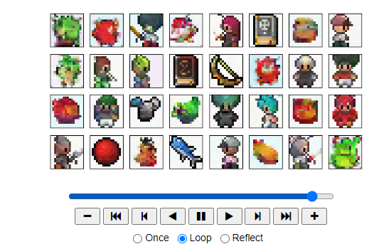
# visualize samples with randomly selected context
plt.clf()
ctx = F.one_hot(torch.randint(0, 5, (32,)), 5).to(device=device).float()
samples, intermediate = sample_ddpm_context(32, ctx)
animation_ddpm_context = plot_sample(intermediate,32,4,save_dir, "ani_run", None, save=False)
HTML(animation_ddpm_context.to_jshtml())
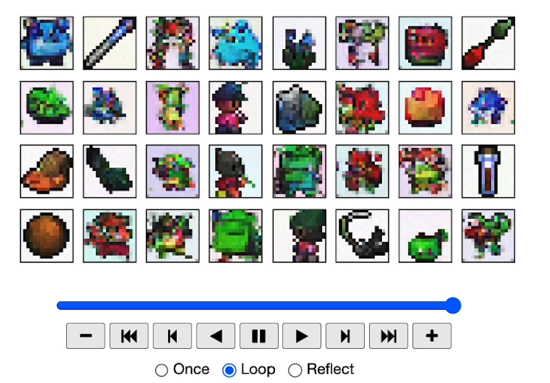
Output
def show_images(imgs, nrow=2):_, axs = plt.subplots(nrow, imgs.shape[0] // nrow, figsize=(4,2 ))axs = axs.flatten()for img, ax in zip(imgs, axs):img = (img.permute(1, 2, 0).clip(-1, 1).detach().cpu().numpy() + 1) / 2ax.set_xticks([])ax.set_yticks([])ax.imshow(img)plt.show()
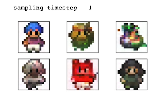
# user defined context
ctx = torch.tensor([# hero, non-hero, food, spell, side-facing[1,0,0,0,0],  [1,0,0,0,0],    [0,0,0,0,1],[0,0,0,0,1],    [0,1,0,0,0],[0,1,0,0,0],[0,0,1,0,0],[0,0,1,0,0],
]).float().to(device)
samples, _ = sample_ddpm_context(ctx.shape[0], ctx)
show_images(samples)
Output
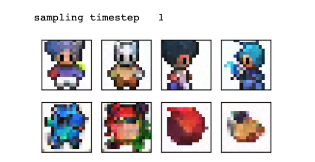
# mix of defined context
ctx = torch.tensor([# hero, non-hero, food, spell, side-facing[1,0,0,0,0],      #human[1,0,0.6,0,0],    [0,0,0.6,0.4,0],  [1,0,0,0,1],  [1,1,0,0,0],[1,0,0,1,0]
]).float().to(device)
samples, _ = sample_ddpm_context(ctx.shape[0], ctx)
show_images(samples)
Output
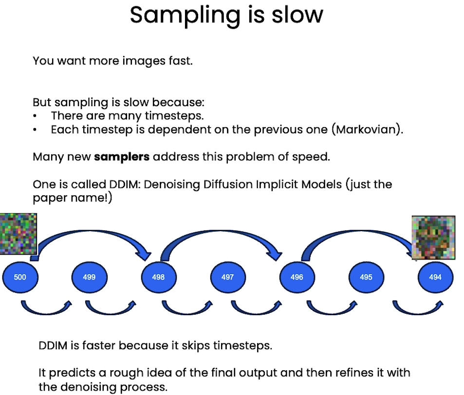
[6] Speeding up
DDIM
DDIM: Denoising Diffusion Implicit Models
from typing import Dict, Tuple
from tqdm import tqdm
import torch
import torch.nn as nn
import torch.nn.functional as F
from torch.utils.data import DataLoader
from torchvision import models, transforms
from torchvision.utils import save_image, make_grid
import matplotlib.pyplot as plt
from matplotlib.animation import FuncAnimation, PillowWriter
import numpy as np
from IPython.display import HTML
from diffusion_utilities import *
Setting Things Up
class ContextUnet(nn.Module):def __init__(self, in_channels, n_feat=256, n_cfeat=10, height=28): # cfeat - context featuressuper(ContextUnet, self).__init__()# number of input channels, number of intermediate feature maps and number of classesself.in_channels = in_channelsself.n_feat = n_featself.n_cfeat = n_cfeatself.h = height #assume h == w. must be divisible by 4, so 28,24,20,16...# Initialize the initial convolutional layerself.init_conv = ResidualConvBlock(in_channels, n_feat, is_res=True)# Initialize the down-sampling path of the U-Net with two levelsself.down1 = UnetDown(n_feat, n_feat) # down1 #[10, 256, 8, 8]self.down2 = UnetDown(n_feat, 2 * n_feat) # down2 #[10, 256, 4, 4]# original: self.to_vec = nn.Sequential(nn.AvgPool2d(7), nn.GELU())self.to_vec = nn.Sequential(nn.AvgPool2d((4)), nn.GELU())# Embed the timestep and context labels with a one-layer fully connected neural networkself.timeembed1 = EmbedFC(1, 2*n_feat)self.timeembed2 = EmbedFC(1, 1*n_feat)self.contextembed1 = EmbedFC(n_cfeat, 2*n_feat)self.contextembed2 = EmbedFC(n_cfeat, 1*n_feat)# Initialize the up-sampling path of the U-Net with three levelsself.up0 = nn.Sequential(nn.ConvTranspose2d(2 * n_feat, 2 * n_feat, self.h//4, self.h//4), nn.GroupNorm(8, 2 * n_feat), # normalize nn.ReLU(),)self.up1 = UnetUp(4 * n_feat, n_feat)self.up2 = UnetUp(2 * n_feat, n_feat)# Initialize the final convolutional layers to map to the same number of channels as the input imageself.out = nn.Sequential(nn.Conv2d(2 * n_feat, n_feat, 3, 1, 1), # reduce number of feature maps #in_channels, out_channels, kernel_size, stride=1, padding=0nn.GroupNorm(8, n_feat), # normalizenn.ReLU(),nn.Conv2d(n_feat, self.in_channels, 3, 1, 1), # map to same number of channels as input)def forward(self, x, t, c=None):"""x : (batch, n_feat, h, w) : input imaget : (batch, n_cfeat) : time stepc : (batch, n_classes) : context label"""# x is the input image, c is the context label, t is the timestep, context_mask says which samples to block the context on# pass the input image through the initial convolutional layerx = self.init_conv(x)# pass the result through the down-sampling pathdown1 = self.down1(x) #[10, 256, 8, 8]down2 = self.down2(down1) #[10, 256, 4, 4]# convert the feature maps to a vector and apply an activationhiddenvec = self.to_vec(down2)# mask out context if context_mask == 1if c is None:c = torch.zeros(x.shape[0], self.n_cfeat).to(x)# embed context and timestepcemb1 = self.contextembed1(c).view(-1, self.n_feat * 2, 1, 1) # (batch, 2*n_feat, 1,1)temb1 = self.timeembed1(t).view(-1, self.n_feat * 2, 1, 1)cemb2 = self.contextembed2(c).view(-1, self.n_feat, 1, 1)temb2 = self.timeembed2(t).view(-1, self.n_feat, 1, 1)#print(f"uunet forward: cemb1 {cemb1.shape}. temb1 {temb1.shape}, cemb2 {cemb2.shape}. temb2 {temb2.shape}")up1 = self.up0(hiddenvec)up2 = self.up1(cemb1*up1 + temb1, down2) # add and multiply embeddingsup3 = self.up2(cemb2*up2 + temb2, down1)out = self.out(torch.cat((up3, x), 1))return out# hyperparameters# diffusion hyperparameters
timesteps = 500
beta1 = 1e-4
beta2 = 0.02# network hyperparameters
device = torch.device("cuda:0" if torch.cuda.is_available() else torch.device('cpu'))
n_feat = 64 # 64 hidden dimension feature
n_cfeat = 5 # context vector is of size 5
height = 16 # 16x16 image
save_dir = './weights/'# training hyperparameters
batch_size = 100
n_epoch = 32
lrate=1e-3
# construct DDPM noise schedule
b_t = (beta2 - beta1) * torch.linspace(0, 1, timesteps + 1, device=device) + beta1
a_t = 1 - b_t
ab_t = torch.cumsum(a_t.log(), dim=0).exp()
ab_t[0] = 1
# construct model
nn_model = ContextUnet(in_channels=3, n_feat=n_feat, n_cfeat=n_cfeat, height=height).to(device)
Fast Sampling
# define sampling function for DDIM
# removes the noise using ddim
def denoise_ddim(x, t, t_prev, pred_noise):ab = ab_t[t]ab_prev = ab_t[t_prev]x0_pred = ab_prev.sqrt() / ab.sqrt() * (x - (1 - ab).sqrt() * pred_noise)dir_xt = (1 - ab_prev).sqrt() * pred_noisereturn x0_pred + dir_xt
# load in model weights and set to eval mode
nn_model.load_state_dict(torch.load(f"{save_dir}/model_31.pth", map_location=device))
nn_model.eval()
print("Loaded in Model without context")
# sample quickly using DDIM
@torch.no_grad()
def sample_ddim(n_sample, n=20):# x_T ~ N(0, 1), sample initial noisesamples = torch.randn(n_sample, 3, height, height).to(device)  # array to keep track of generated steps for plottingintermediate = [] step_size = timesteps // nfor i in range(timesteps, 0, -step_size):print(f'sampling timestep {i:3d}', end='\r')# reshape time tensort = torch.tensor([i / timesteps])[:, None, None, None].to(device)eps = nn_model(samples, t)    # predict noise e_(x_t,t)samples = denoise_ddim(samples, i, i - step_size, eps)intermediate.append(samples.detach().cpu().numpy())intermediate = np.stack(intermediate)return samples, intermediate
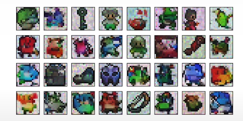
# visualize samples
plt.clf()
samples, intermediate = sample_ddim(32, n=25)
animation_ddim = plot_sample(intermediate,32,4,save_dir, "ani_run", None, save=False)
HTML(animation_ddim.to_jshtml())
Output
# load in model weights and set to eval mode
nn_model.load_state_dict(torch.load(f"{save_dir}/context_model_31.pth", map_location=device))
nn_model.eval()
print("Loaded in Context Model")
# fast sampling algorithm with context
@torch.no_grad()
def sample_ddim_context(n_sample, context, n=20):# x_T ~ N(0, 1), sample initial noisesamples = torch.randn(n_sample, 3, height, height).to(device)  # array to keep track of generated steps for plottingintermediate = [] step_size = timesteps // nfor i in range(timesteps, 0, -step_size):print(f'sampling timestep {i:3d}', end='\r')# reshape time tensort = torch.tensor([i / timesteps])[:, None, None, None].to(device)eps = nn_model(samples, t, c=context)    # predict noise e_(x_t,t)samples = denoise_ddim(samples, i, i - step_size, eps)intermediate.append(samples.detach().cpu().numpy())intermediate = np.stack(intermediate)return samples, intermediate
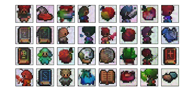
# visualize samples
plt.clf()
ctx = F.one_hot(torch.randint(0, 5, (32,)), 5).to(device=device).float()
samples, intermediate = sample_ddim_context(32, ctx)
animation_ddpm_context = plot_sample(intermediate,32,4,save_dir, "ani_run", None, save=False)
HTML(animation_ddpm_context.to_jshtml())
Output
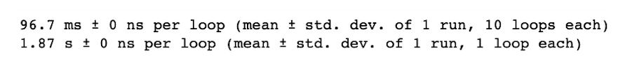
Compare DDPM, DDIM speed
# helper function; removes the predicted noise (but adds some noise back in to avoid collapse)
def denoise_add_noise(x, t, pred_noise, z=None):if z is None:z = torch.randn_like(x)noise = b_t.sqrt()[t] * zmean = (x - pred_noise * ((1 - a_t[t]) / (1 - ab_t[t]).sqrt())) / a_t[t].sqrt()return mean + noise
# sample using standard algorithm
@torch.no_grad()
def sample_ddpm(n_sample, save_rate=20):# x_T ~ N(0, 1), sample initial noisesamples = torch.randn(n_sample, 3, height, height).to(device)  # array to keep track of generated steps for plottingintermediate = [] for i in range(timesteps, 0, -1):print(f'sampling timestep {i:3d}', end='\r')# reshape time tensort = torch.tensor([i / timesteps])[:, None, None, None].to(device)# sample some random noise to inject back in. For i = 1, don't add back in noisez = torch.randn_like(samples) if i > 1 else 0eps = nn_model(samples, t)    # predict noise e_(x_t,t)samples = denoise_add_noise(samples, i, eps, z)if i % save_rate ==0 or i==timesteps or i<8:intermediate.append(samples.detach().cpu().numpy())intermediate = np.stack(intermediate)return samples, intermediate
%timeit -r 1 sample_ddim(32, n=25)
%timeit -r 1 sample_ddpm(32, )
Output
后记
经过2天的时间,大概2小时,完成这门课的学习。代码是给定的,所以没有自己写代码的过程,但是让我对扩散模型有了一定的了解,想要更深入的理解扩散模型,还是需要阅读论文和相关资料。这门课仅仅是入门课。
相关文章:
从零开始学习Diffusion Models: Sharon Zhou
How Diffusion Models Work 本文是 https://www.deeplearning.ai/short-courses/how-diffusion-models-work/ 这门课程的学习笔记。 文章目录 How Diffusion Models WorkWhat you’ll learn in this course [1] Intuition[2] SamplingSetting Things UpSamplingDemonstrate i…...
全天候购药系统(微信小程序+web后台管理)
PurchaseApplet 全天候购药系统(微信小程序web后台管理) 传统线下购药方式存在无法全天候向用户提供购药服务,无法随时提供诊疗服务等问题。为此,运用软件工程开发规范,充分调研建立需求模型,编写开发文档…...
)
L2-003 月饼(Java)
月饼是中国人在中秋佳节时吃的一种传统食品,不同地区有许多不同风味的月饼。现给定所有种类月饼的库存量、总售价、以及市场的最大需求量,请你计算可以获得的最大收益是多少。 注意:销售时允许取出一部分库存。样例给出的情形是这样的&#…...
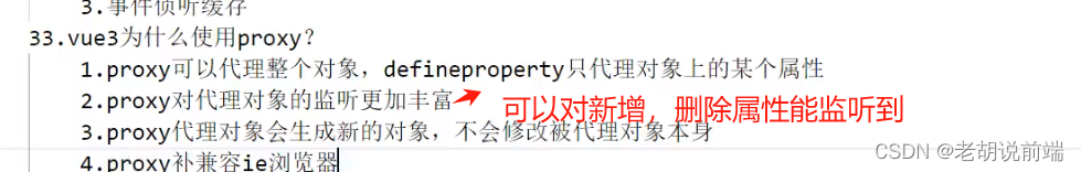
vue面试--101, 1vue3为啥比vue2好 2 vue3为什么使用proxy
1vue3为啥比vue2好 2 vue3为什么使用proxy...
【sgPhotoPlayer】自定义组件:图片预览,支持点击放大、缩小、旋转图片
特性: 支持设置初始索引值支持显示标题、日期、大小、当前图片位置支持无限循环切换轮播支持鼠标滑轮滚动、左右键、上下键、PageUp、PageDown、Home、End操作切换图片支持Esc关闭窗口 sgPhotoPlayer源码 <template><div :class"$options.name"…...
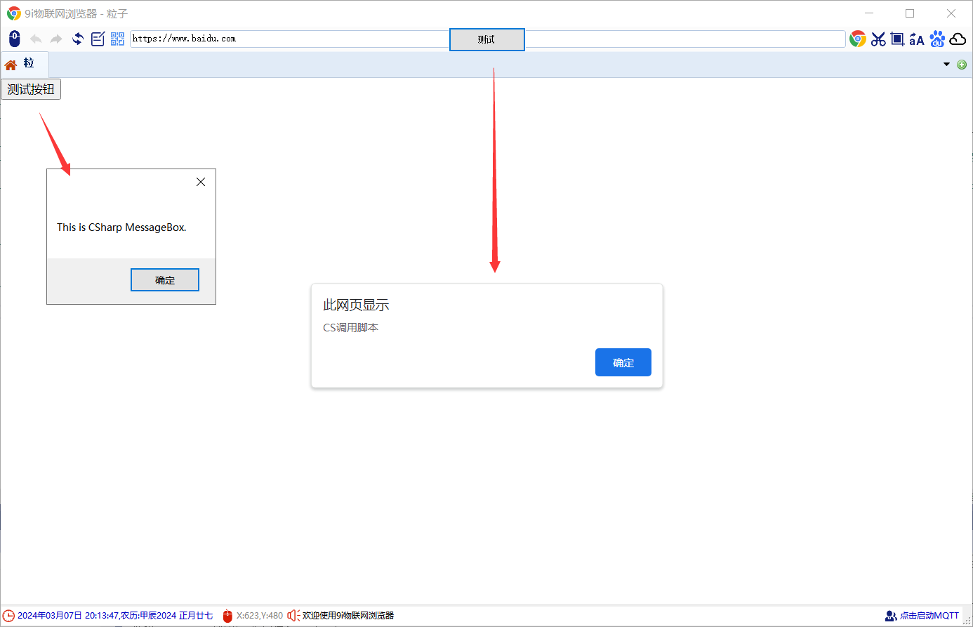
cefsharp(winForm)调用js脚本,js脚本调用c#方法
本博文针对js-csharp交互(相互调用的应用) (一)、js调用c#方法 1.1 类名称:cs_js_obj public class cs_js_obj{//注意,js调用C#,不一定在主线程上调用的,需要用SynchronizationContext来切换到主线程//private System.Threading.SynchronizationContext context;//…...
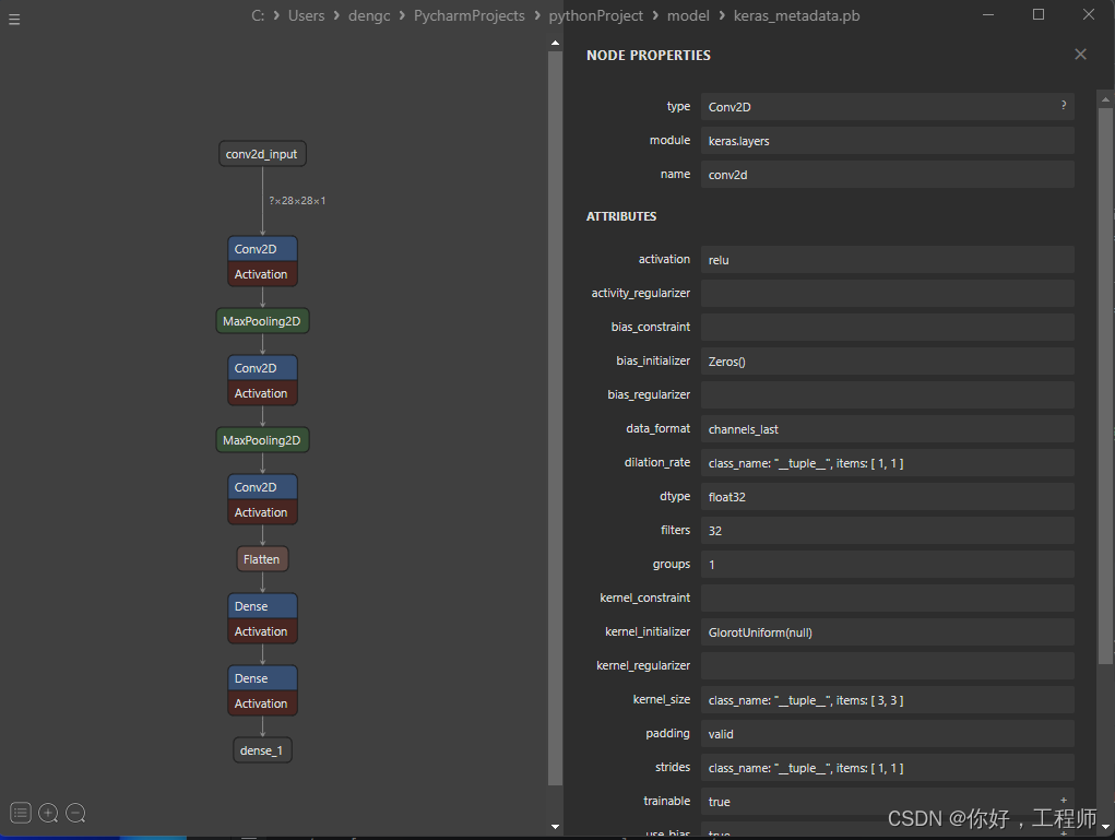
Tensorflow实现手写数字识别
模型架构 具有10个神经元,对应10个类别(0-9的数字)。使用softmax激活函数,对多分类问题进行概率归一化。输出层 (Dense):具有64个神经元。激活函数为ReLU。全连接层 (Dense):将二维数据展平成一维,为全连接层做准备。展…...

谈谈杭州某小公司面试的经历
#面试#本人bg211本,一段实习,前几天面了杭州某小厂公司,直接给我干无语了! 1、先介绍介绍你自己,我说了我的一个情况。 2、没获奖和竞赛经历吗?我说确实没有呢,面试官叹气了一下,只是…...
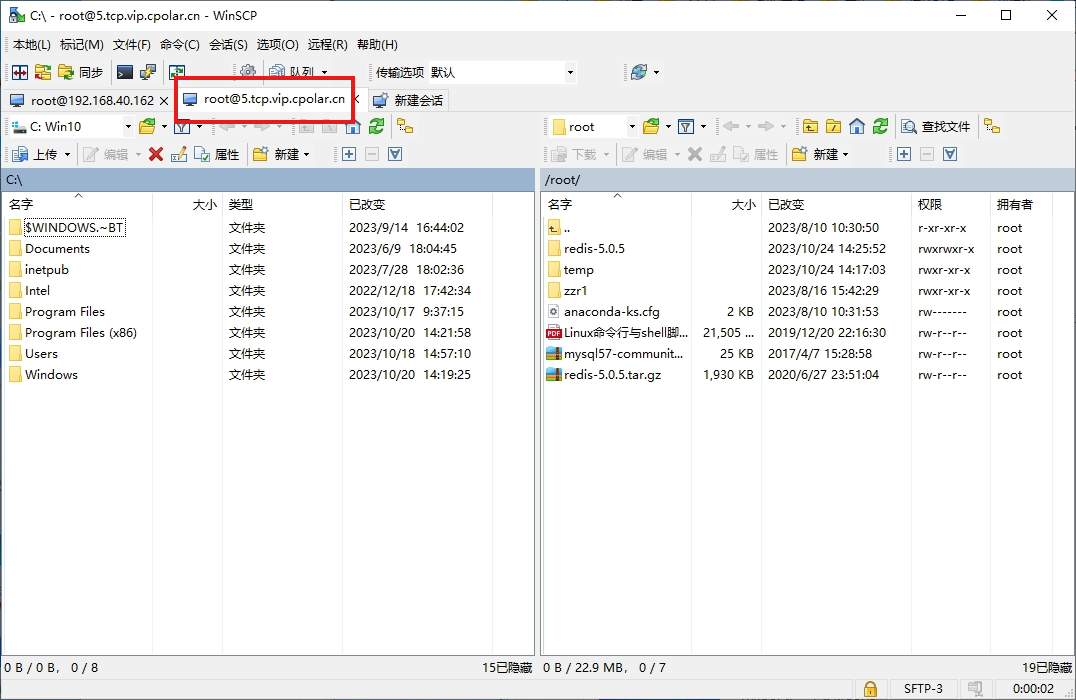
如何使用WinSCP结合Cpolar实现公网远程访问内网Linux服务器
文章目录 1. 简介2. 软件下载安装:3. SSH链接服务器4. WinSCP使用公网TCP地址链接本地服务器5. WinSCP使用固定公网TCP地址访问服务器 1. 简介 Winscp是一个支持SSH(Secure SHell)的可视化SCP(Secure Copy)文件传输软件,它的主要功能是在本地与远程计…...

6. 互质
互质 互质 互质 每次测试的时间限制: 3 秒 每次测试的时间限制:3 秒 每次测试的时间限制:3秒 每次测试的内存限制: 256 兆字节 每次测试的内存限制:256 兆字节 每次测试的内存限制:256兆字节 题目描述 给定…...

微信小程序(五十一)页面背景(全屏)
注释很详细,直接上代码 上一篇 新增内容: 1.页面背景的基本写法 2.去除默认上标题实习全屏背景 3. 背景适配细节 源码: index.wxss page{/* 背景链接 */background-image: url(https://pic3.zhimg.com/v2-a76bafdecdacebcc89b5d4f351a53e6a_…...
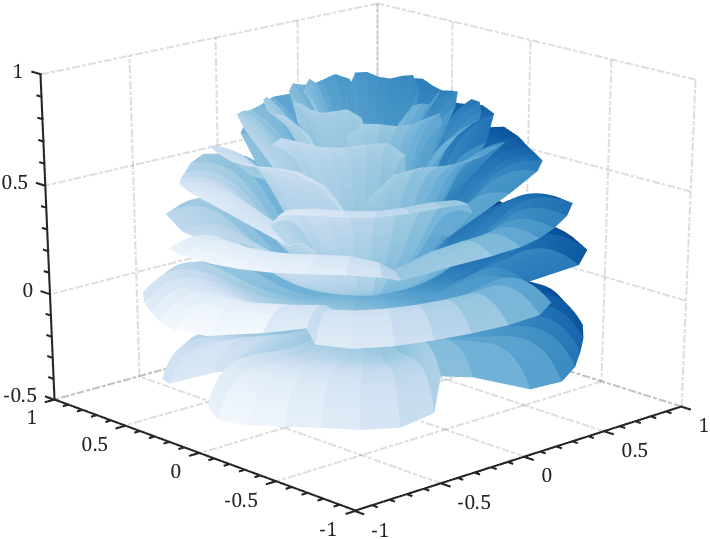
MATLAB | MATLAB版玫瑰祝伟大女性节日快乐!!
妇女节到了,这里祝全体伟大的女性,节日快乐,事业有成,万事胜意。 作为MATLAB爱好者,这里还是老传统画朵花叭,不过感觉大部分样式的花都画过了,这里将一段很古老的2012年的html玫瑰花代码转成MA…...
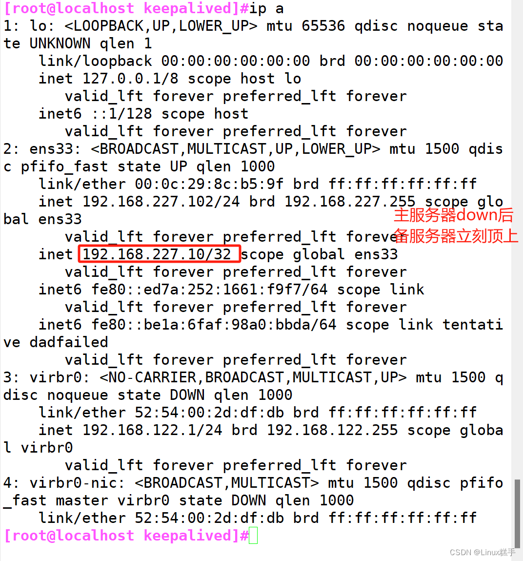
LVS+Keepalived 高可用集群
目录 一.Keepalived工具介绍 1.用户空间核心组件: (1)vrrp stack:VIP消息通告 (2)checkers:监测real server(简单来说 就是监控后端真实服务器的服务) (…...
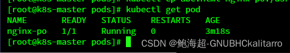
Linux:kubernetes(k8s)探针ReadinessProbe的使用(9)
本章yaml文件是根据之前文章迭代修改过来的 先将之前的pod删除,然后使用下面这个yaml进行生成pod apiVersion: v1 # api文档版本 kind: Pod # 资源对象类型 metadata: # pod相关的元数据,用于描述pod的数据name: nginx-po # pod名称labels: # pod的标…...
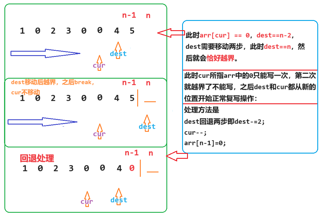
专题一 - 双指针 - leetcode 1089. 复写零 - 简单难度
leetcode 1089. 复写零 leetcode 1089. 复写零 | 简单难度1. 题目详情1. 原题链接2. 基础框架 2. 解题思路1. 题目分析2. 算法原理3. 时间复杂度 3. 代码实现4. 知识与收获 leetcode 1089. 复写零 | 简单难度 1. 题目详情 给你一个长度固定的整数数组 arr ,请你将…...
深入浅出(二)MVVM
MVVM 1. 简介2. 示例 1. 简介 2. 示例 示例下载地址:https://download.csdn.net/download/qq_43572400/88925141 创建C# WPF应用(.NET Framework)工程,WpfApp1 添加程序集 GalaSoft.MvvmLight 创建ViewModel文件夹,并创建MainWindowV…...
A题思路)
2023年第三届中国高校大数据挑战赛(第二场)A题思路
竞赛时间 (1)报名时间:即日起至2024年3月8日 (2)比赛时间:2024年3月9日8:00至2024年3月12日20:00 (3)成绩公布:2024年4月30日前 赛题方向:大数据统计分析 …...

数据挖掘:
一.数据仓库概述: 1.1数据仓库概述 1.1.1数据仓库定义 数据仓库是一个用于支持管理决策的、面向主题、集成、相对稳定且反映历史变化的数据集合。 1.1.2数据仓库四大特征 集成性(Integration): 数据仓库集成了来自多个不同来源…...
NDK,Jni
使用 NDK(Native Development Kit)意味着在 Android 应用程序中集成 C/C 代码。通常情况下,Android 应用程序主要使用 Java 或 Kotlin 编写,但有时候需要使用 C/C 来实现一些特定的功能或性能优化。 NDK 提供了一组工具和库&…...

Java实战:Spring Boot整合Canal与RabbitMQ实时监听数据库变更并高效处理
引言 在现代微服务架构中,数据的变化往往需要及时地传播给各个相关服务,以便于同步更新状态或触发业务逻辑。Canal作为一个开源的MySQL binlog订阅和消费组件,能够帮助我们实时捕获数据库的增删改操作。而RabbitMQ作为一款消息中间件&#x…...

Kubernetes智能运维助手:基于LLM的kube-copilot实战指南
1. 项目概述:当Kubernetes遇上AI副驾驶如果你和我一样,每天都要和Kubernetes集群打交道,那你肯定对下面这些场景不陌生:凌晨三点被告警叫醒,面对一个不断重启的Pod,需要手动执行一串kubectl describe、kube…...

终极指南:3分钟实现GitHub全界面中文化,彻底消除语言障碍
终极指南:3分钟实现GitHub全界面中文化,彻底消除语言障碍 【免费下载链接】github-chinese GitHub 汉化插件,GitHub 中文化界面。 (GitHub Translation To Chinese) 项目地址: https://gitcode.com/gh_mirrors/gi/github-chinese GitH…...

离散化离散化差分
数组开不了1e9,但是好在坐标点会很分散,那么相当于将点“挤到”1-n的位置,一个位置映射了一个坐标点,排序后,坐标的相对位置并不发生改变,离散化由此得来。#include<bits/stdc.h> #define int long l…...

ARM调试器AXD核心功能与实战技巧详解
1. ARM调试器AXD核心功能解析作为一名嵌入式开发工程师,我使用AXD调试器已有八年时间。这款ARM官方调试工具在处理器底层调试方面表现出色,尤其擅长处理各种复杂的内存访问问题和执行流程异常。AXD最突出的特点是其精细化的执行控制和全面的调试信息展示…...

算法时代,技术人如何寻找自己的 “人生硬代码”
前言:我们优化了代码,却常常忽略了人生系统在 AI 日新月异、信息密度持续升高的时代,很多人比过去更忙,却也更容易迷茫。作为技术人,我们熟悉架构设计、性能优化、代码重构和系统调优。面对一个工程问题时,…...

国产多模态大模型“刘知远”:技术原理、实战应用与未来展望
国产多模态大模型“刘知远”:技术原理、实战应用与未来展望 引言 在人工智能浪潮中,多模态大模型正成为推动AGI(通用人工智能)发展的关键引擎。当全球目光聚焦于GPT-4、DALL-E等明星模型时,国产力量也在悄然崛起。其中…...
)
告别JSON臃肿:手把手教你用MessagePack为C++微服务瘦身(附性能对比)
告别JSON臃肿:手把手教你用MessagePack为C微服务瘦身(附性能对比) 在当今高性能后端服务开发中,微服务架构已成为主流选择。然而,随着服务规模的扩大,服务间通信的数据量急剧增长,传统的JSON序列…...

基于React与Docker构建可定制个人仪表盘:homepage项目实战指南
1. 项目概述:一个现代、轻量的个人仪表盘如果你和我一样,每天上班第一件事就是打开十几个浏览器标签页,在邮箱、项目管理工具、服务器监控、待办清单、常用文档之间来回切换,那么你一定能理解那种“数字工作台”杂乱无章带来的烦躁…...

解读民法典基本规定第十条
民法典: 第一编 总则,第一章 基本规定 第十条 处理民事纠纷,应当依照法律;法律没有规定的,可以适用习惯,但是不得违背公序良俗。 一句话核心 先按国法判,国法没写明白,就按当地老规矩、民间习俗…...

C-Eval中文基准测试到底准不准?3轮人工校验+5类对抗样本验证,真相令人震惊
更多请点击: https://intelliparadigm.com 第一章:C-Eval中文基准测试到底准不准?3轮人工校验5类对抗样本验证,真相令人震惊 C-Eval 作为当前主流的中文大模型评测基准,长期被用于学术论文与工业选型,但其…...