LLM大模型可视化-以nano-gpt为例
内容整理自:LLM 可视化 --- LLM Visualization (bbycroft.net)![]() https://bbycroft.net/llm
https://bbycroft.net/llm
Introduction 介绍
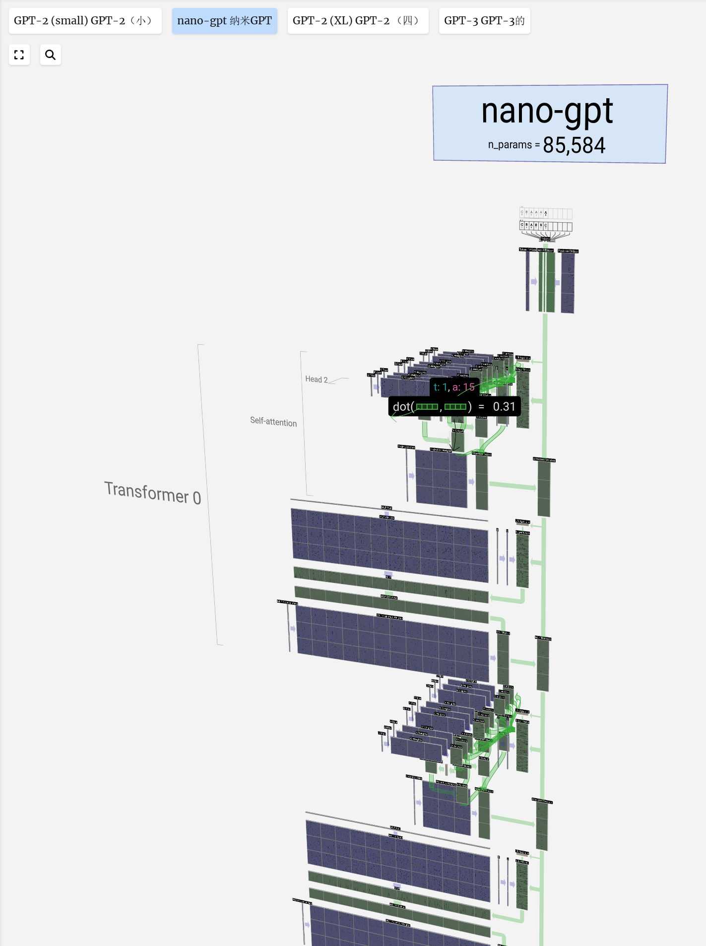
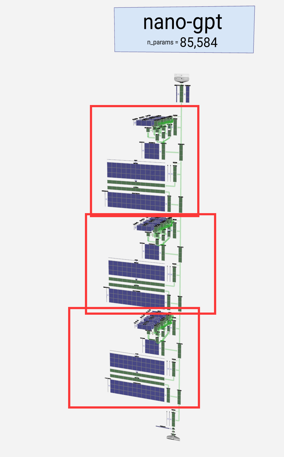
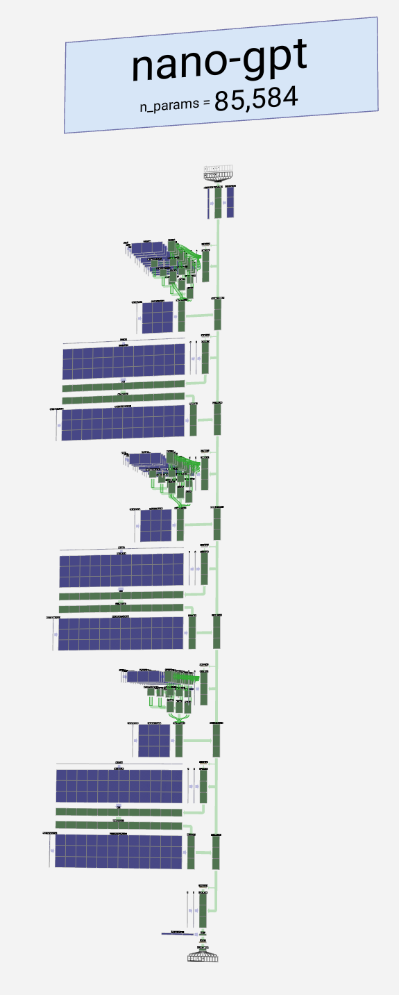
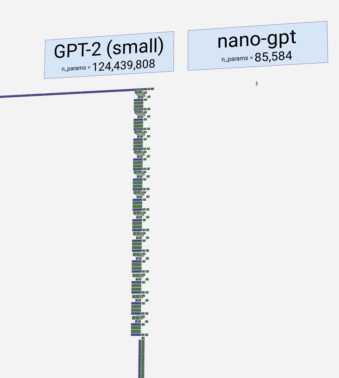
Welcome to the walkthrough of the GPT large language model! Here we'll explore the model nano-gpt, with a mere 85,000 parameters.
欢迎来到 GPT 大型语言模型的演练!在这里,我们将探索只有 85,000 个参数的 nano-gpt 模型。
Its goal is a simple one: take a sequence of six letters:
它的目标很简单:取六个字母的序列:
and sort them in alphabetical order, i.e. to "ABBBCC".
并按字母顺序排序,即“ABBBCC”。
We call each of these letters a token, and the set of the model's different tokens make up its vocabulary:
我们将这些字母中的每一个称为标记,模型的不同标记集构成了它的词汇表:
| token 令牌 | A | B | C |
|---|---|---|---|
| index 索引 | 0 | 1 | 2 |
From this table, each token is assigned a number, its token index. And now we can enter this sequence of numbers into the model:
在此表中,每个令牌都分配了一个数字,即其令牌索引。现在我们可以将这个数字序列输入到模型中:
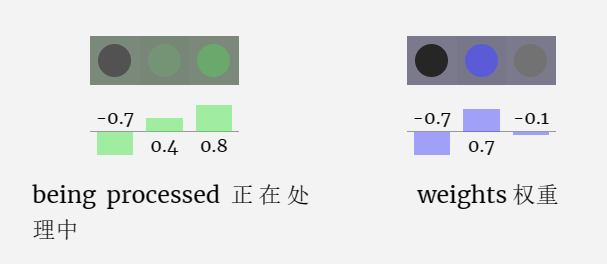
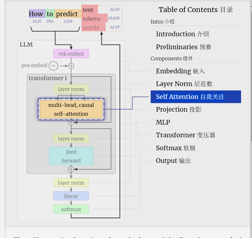
在 3D 视图中,每个绿色单元格代表一个正在处理的数字,每个蓝色单元格代表一个权重。
序列中的每个数字首先转换为一个 48 元素向量(为此特定模型选择的大小)。这称为嵌入。
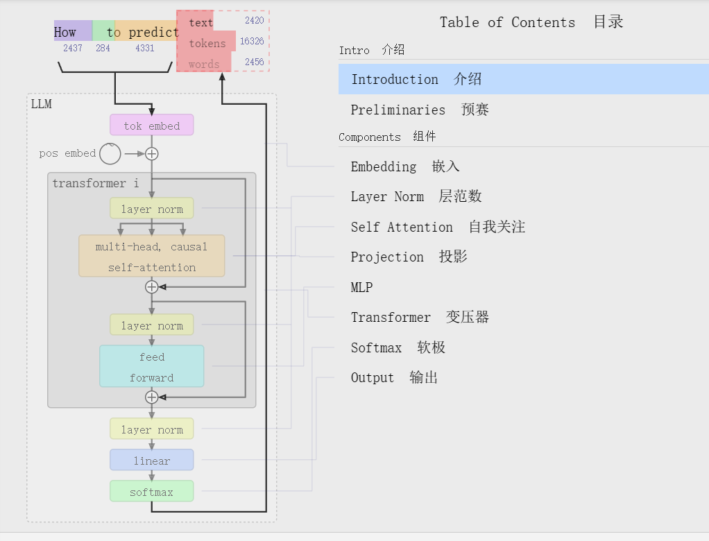
The embedding is then passed through the model, going through a series of layers, called transformers, before reaching the bottom.
然后,嵌入通过模型,经过一系列层,称为transformers,然后到达底部。
The embedding is then passed through the model, going through a series of layers, called transformers, before reaching the bottom.
然后,嵌入通过模型,经过一系列层,称为转换器,然后到达底部。
So what's the output? A prediction of the next token in the sequence. So at the 6th entry, we get probabilities that the next token is going to be 'A', 'B', or 'C'.
那么输出是什么?对序列中下一个标记的预测。因此,在第 6 个条目中,我们得到下一个代币将是“A”、“B”或“C”的概率。
In this case, the model is pretty sure it's going to be 'A'. Now, we can feed this prediction back into the top of the model, and repeat the entire process.
在本例中,模型非常确定它将是“A”。现在,我们可以将这个预测反馈到模型的顶部,并重复整个过程。
Preliminaries 准备工作
Before we delve into the algorithm's intricacies, let's take a brief step back.
在我们深入研究算法的复杂性之前,让我们先退后一步。
This guide focuses on inference, not training, and as such is only a small part of the entire machine-learning process. In our case, the model's weights have been pre-trained, and we use the inference process to generate output. This runs directly in your browser.
本指南侧重于推理,而不是训练,因此只是整个机器学习过程的一小部分。在我们的例子中,模型的权重已经过预训练,我们使用推理过程来生成输出。这将直接在您的浏览器中运行。
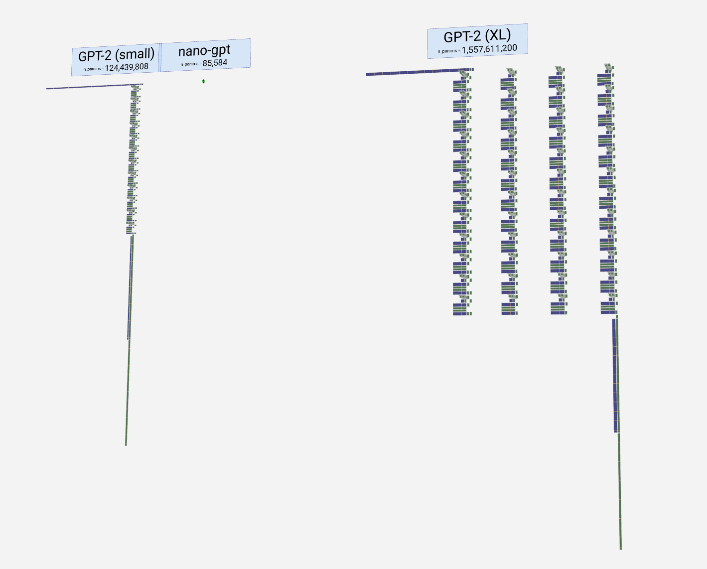
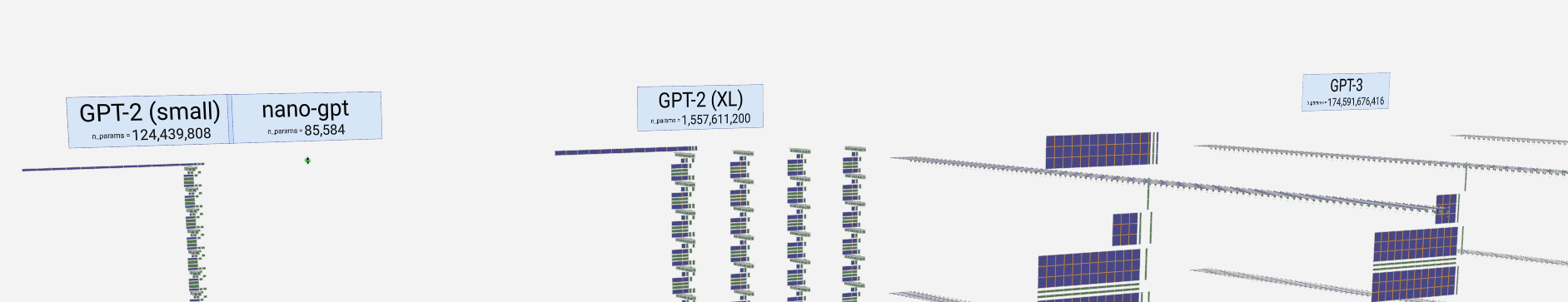
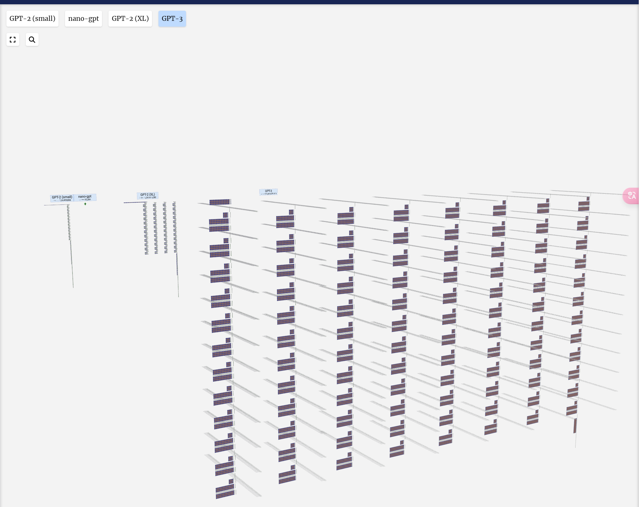
The model showcased here is part of the GPT (generative pre-trained transformer) family, which can be described as a "context-based token predictor". OpenAI introduced this family in 2018, with notable members such as GPT-2, GPT-3, and GPT-3.5 Turbo, the latter being the foundation of the widely-used ChatGPT. It might also be related to GPT-4, but specific details remain unknown.
这里展示的模型是 GPT(生成式预训练transformer)系列的一部分,可以描述为“基于上下文的令牌预测器”。OpenAI 于 2018 年推出了这个系列,其中包括 GPT-2、GPT-3 和 GPT-3.5 Turbo 等著名成员,后者是广泛使用的 ChatGPT 的基础。它也可能与 GPT-4 有关,但具体细节仍然未知。
This guide was inspired by the minGPT GitHub project, a minimal GPT implementation in PyTorch created by Andrej Karpathy. His YouTube series Neural Networks: Zero to Hero and the minGPT project have been invaluable resources in the creation of this guide. The toy model featured here is based on one found within the minGPT project.
本指南的灵感来自 minGPT GitHub 项目,这是 Andrej Karpathy 在 PyTorch 中创建的最小 GPT 实现。他的 YouTube 系列《 Neural Networks: Zero to Hero 》和 minGPT 项目是创建本指南的宝贵资源。这里展示的玩具模型是基于 minGPT 项目中的一个。
Alright, let's get started!
好了,让我们开始吧!
Components 组件
Embedding 嵌入
We saw previously how the tokens are mapped to a sequence of integers using a simple lookup table. These integers, the token indices, are the first and only time we see integers in the model. From here on out, we're using floats (decimal numbers).
我们之前看到如何使用简单的查找表将标记映射到整数序列。这些整数,即标记索引,是我们第一次也是唯一一次在模型中看到整数。从现在开始,我们将使用浮点数(十进制数)。
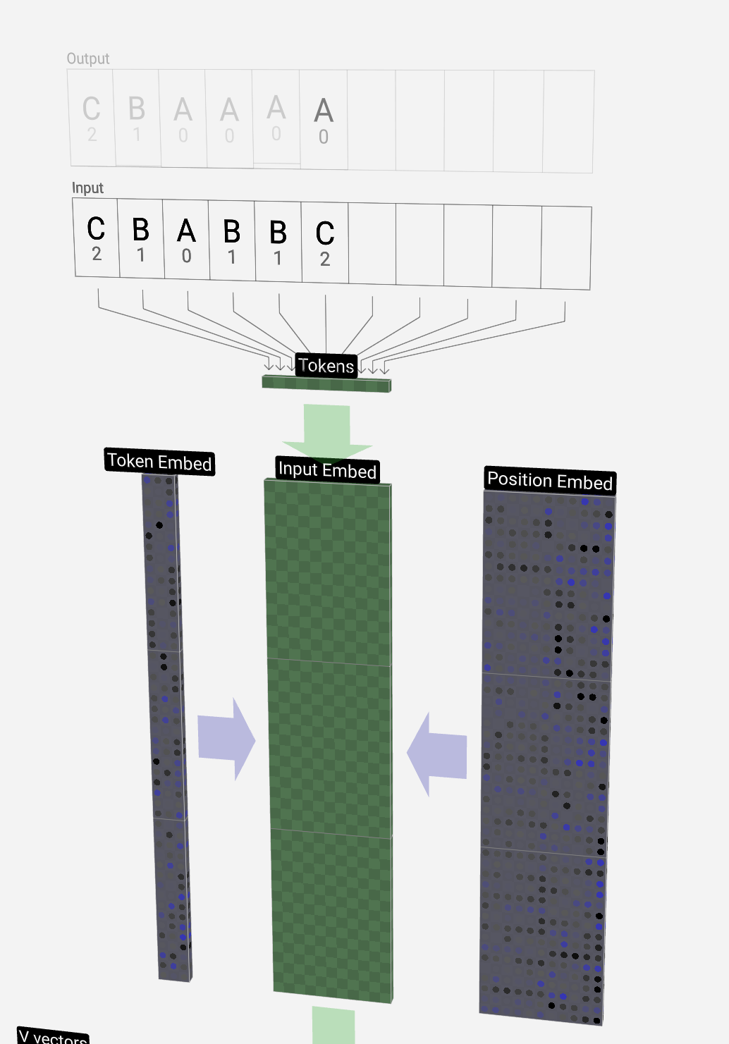
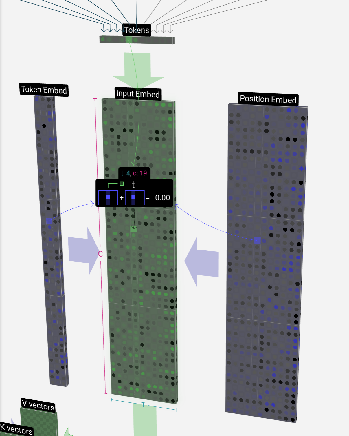
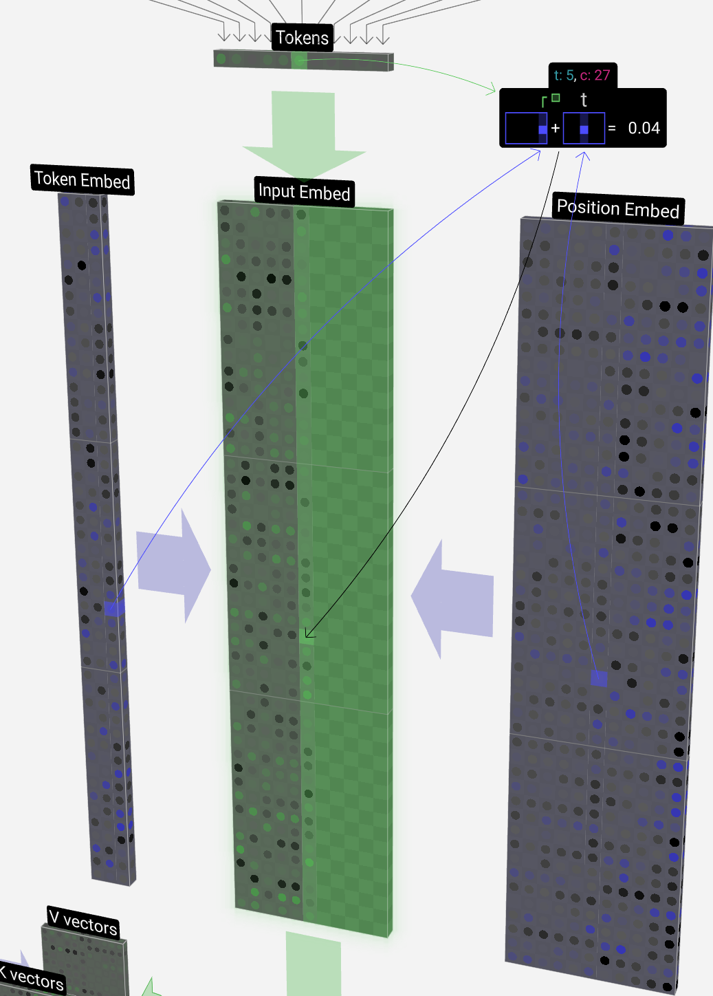
Let's take a look at how the 4th token (index 3) is used to generate the 4th column vector of our input embedding.
让我们看一下如何使用第 4 个标记(索引 3)来生成输入嵌入的第 4 列向量。
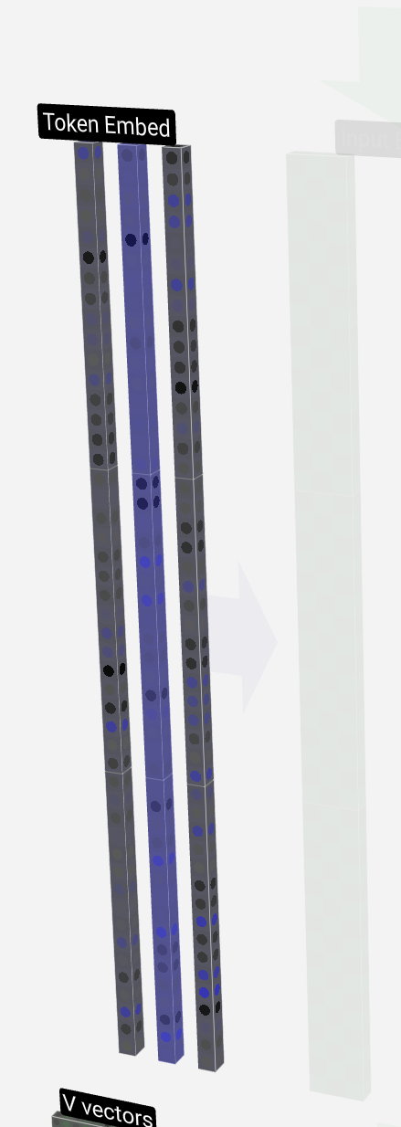
We use the token index (in this case B = 1) to select the 2nd column of the token embedding matrix on the left. Note we're using 0-based indexing here, so the first column is at index 0.
我们使用令牌索引(在本例中为 B = 1)选择左侧令牌嵌入矩阵的第 2 列。请注意,我们在这里使用的是从 0 开始的索引,因此第一列位于索引 0 处。
This produces a column vector of size C = 48, which we describe as the token embedding.
这将生成一个大小为 C = 48 的列向量,我们将其描述为标记嵌入。
And since we're looking at our token B in the 4th position (t = 3), we'll take the 4th column of the position embedding matrix.
由于我们查看的是第 4 个位置的标记 B(t = 3),因此我们将采用位置嵌入矩阵的第 4 列。
This also produces a column vector of size C = 48, which we describe as the position embedding.
这也会产生一个大小为 C = 48 的列向量,我们将其描述为位置嵌入。
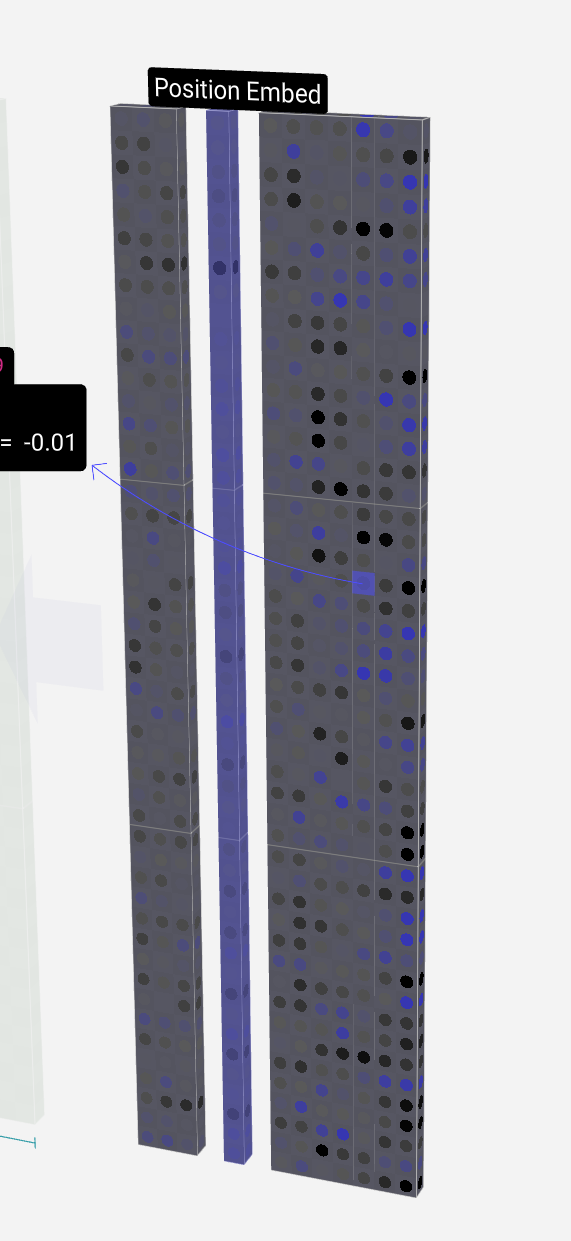
Note that both of these position and token embeddings are learned during training (indicated by their blue color).
请注意,这两个位置和标记嵌入都是在训练期间学习的(由它们的蓝色表示)。
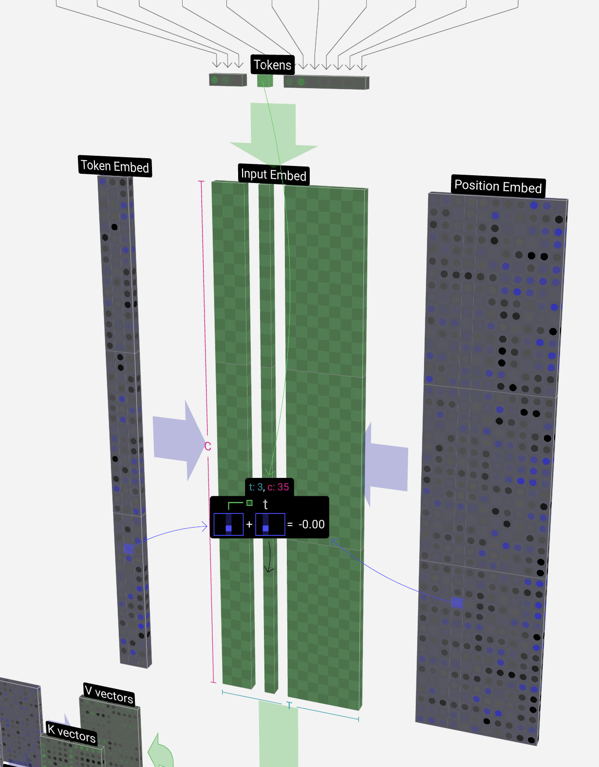
Now that we have these two column vectors, we simply add them together to produce another column vector of size C = 48.
现在我们有了这两个列向量,我们只需将它们相加即可生成另一个大小为 C = 48 的列向量。
We now run this same process for all of the tokens in the input sequence, creating a set of vectors which incorporate both the token values and their positions.
现在,我们对输入序列中的所有标记运行相同的过程,创建一组包含标记值及其位置的向量。
We see that running this process for all the tokens in the input sequence produces a matrix of size T x C. The T stands for time, i.e., you can think of tokens later in the sequence as later in time. The C stands for channel, but is also referred to as "feature" or "dimension" or "embedding size". This length, C, is one of the several "hyperparameters" of the model, and is chosen by the designer to in a tradeoff between model size and performance.
我们看到,对输入序列中的所有标记运行此过程会产生大小为 T x C 的矩阵。T 代表时间,即您可以将序列中后面的标记视为时间的后面。C 代表通道,但也被称为“特征”或“维度”或“嵌入大小”。这个长度 C 是模型的几个“超参数”之一,由设计人员选择,以在模型大小和性能之间进行权衡。
This matrix, which we'll refer to as the input embedding is now ready to be passed down through the model. This collection of T columns each of length C will become a familiar sight throughout this guide.
这个矩阵,我们称之为输入嵌入,现在已经准备好通过模型传递了。这组 T 列,每个柱子的长度为 C,将成为本指南中熟悉的景象。
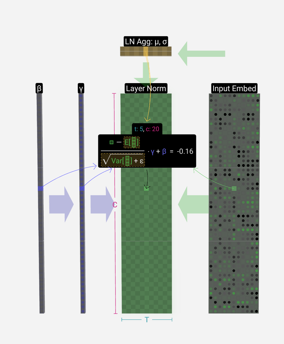
Layer Norm 层归一化
The input embedding matrix from the previous section is the input to our first Transformer block.
上一节中的输入嵌入矩阵是第一个 Transformer 模块的输入。
The first step in the Transformer block is to apply layer normalization to this matrix. This is an operation that normalizes the values in each column of the matrix separately.
Transformer 模块的第一步是将层归一化应用于此矩阵。这是分别对矩阵每列中的值进行归一化的操作。
Normalization is an important step in the training of deep neural networks, and it helps improve the stability of the model during training.
归一化是深度神经网络训练中的重要步骤,有助于提高模型在训练过程中的稳定性。
We can regard each column separately, so let's focus on the 4th column (t = 3) for now.
我们可以分别查看每列,所以现在让我们关注第 4 列 (t = 3)。
The goal is to make the average value in the column equal to 0 and the standard deviation equal to 1. To do this, we find both of these quantities (mean (μ) & std dev (σ)) for the column and then subtract the average and divide by the standard deviation.
目标是使列中的平均值等于 0,标准差等于 1。为此,我们找到列的这两个量(平均值(μ)和标准开发(σ)),然后减去平均值并除以标准差。
The notation we use here is E[x] for the average and Var[x] for the variance (of the column of length C). The variance is simply the standard deviation squared. The epsilon term (ε = 1×10⁻⁵) is there to prevent division by zero.
我们在这里使用的符号是 E[x] 表示平均值,Var[x] 表示方差(长度为 C 的列)。方差只是标准差的平方。epsilon 项 (ε = 1×10 -5 ) 是为了防止除以零。
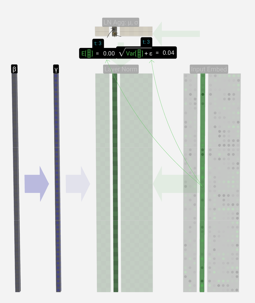
We compute and store these values in our aggregation layer since we're applying them to all values in the column.
我们计算这些值并将其存储在聚合层中,因为我们将它们应用于列中的所有值。
Finally, once we have the normalized values, we multiply each element in the column by a learned weight (γ) and then add a bias (β) value, resulting in our normalized values.
最后,一旦我们有了归一化值,我们将列中的每个元素乘以学习的权重 (γ),然后添加一个偏差 (β) 值,从而得到我们的归一化值。
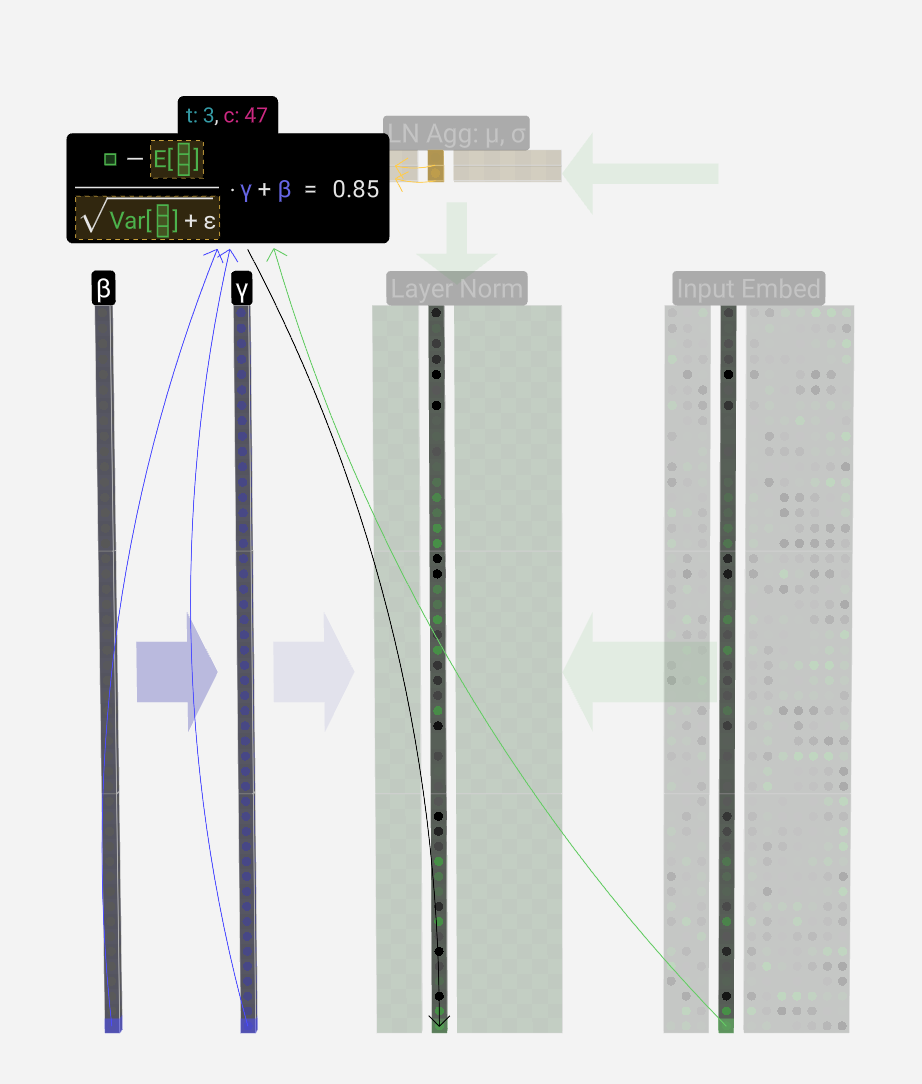
We run this normalization operation on each column of the input embedding matrix, and the result is the normalized input embedding, which is ready to be passed into the Self-Attention layer.
我们对输入嵌入矩阵的每一列运行此归一化操作,结果是归一化输入嵌入,该嵌入已准备好传递到自注意力层。
Self Attention 自注意力
The self-attention layer is perhaps the heart of the Transformer and of GPT. It's the phase where the columns in our input embedding matrix "talk" to each other. Up until now, and in all other phases, the columns can be regarded independently.
自我关注层可能是 Transformer 和 GPT 的核心。这是输入嵌入矩阵中的列相互“对话”的阶段。到目前为止,在所有其他阶段,这些柱子都可以独立地看待。
The self-attention layer is made up of several heads, and we'll focus on one of them for now.
自我关注层由几个头组成,我们现在将重点放在其中一个头上。
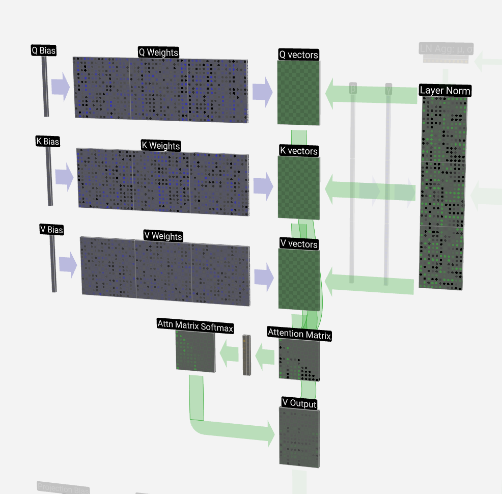
The first step is to produce three vectors for each of the T columns from the normalized input embedding matrix. These vectors are the Q, K, and V vectors:
第一步是从归一化输入嵌入矩阵中为每个 T 列生成三个向量。这些向量是 Q、K 和 V 向量:
- Q: Query vector 问:查询向量
- K: Key vector K:关键向量
- V: Value vector V:价值向量
To produce one of these vectors, we perform a matrix-vector multiplication with a bias added. Each output cell is some linear combination of the input vector. E.g. for the Q vectors, this is done with a dot product between a row of the Q-weight matrix and a column of the input matrix.
为了产生这些向量之一,我们执行矩阵向量乘法,并添加偏差。每个输出单元都是输入向量的线性组合。例如,对于 Q 向量,这是通过 Q 权重矩阵的一行和输入矩阵的一列之间的点积来完成的。
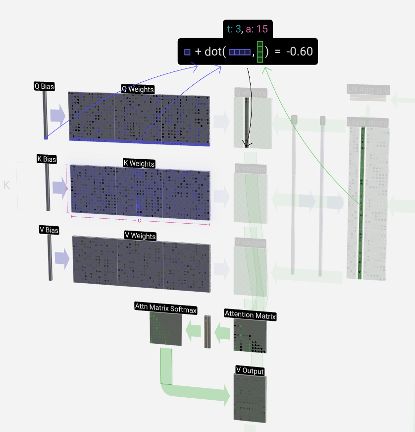
The dot product operation, which we'll see a lot of, is quite simple: We pair each element from the first vector with the corresponding element from the second vector, multiply the pairs together and then add the results up.
点积运算非常简单:我们将第一个向量中的每个元素与第二个向量中的相应元素配对,将这些对相乘,然后将结果相加。
This is a general and simple way of ensuring each output element can be influenced by all the elements in the input vector (where that influence is determined by the weights). Hence its frequent appearance in neural networks.
这是一种通用且简单的方法,可确保每个输出元素都可以受到输入向量中所有元素的影响(其中该影响由权重决定)。因此,它经常出现在神经网络中。
We repeat this operation for each output cell in the Q, K, V vectors:
我们对 Q、K、V 向量中的每个输出单元重复此操作:
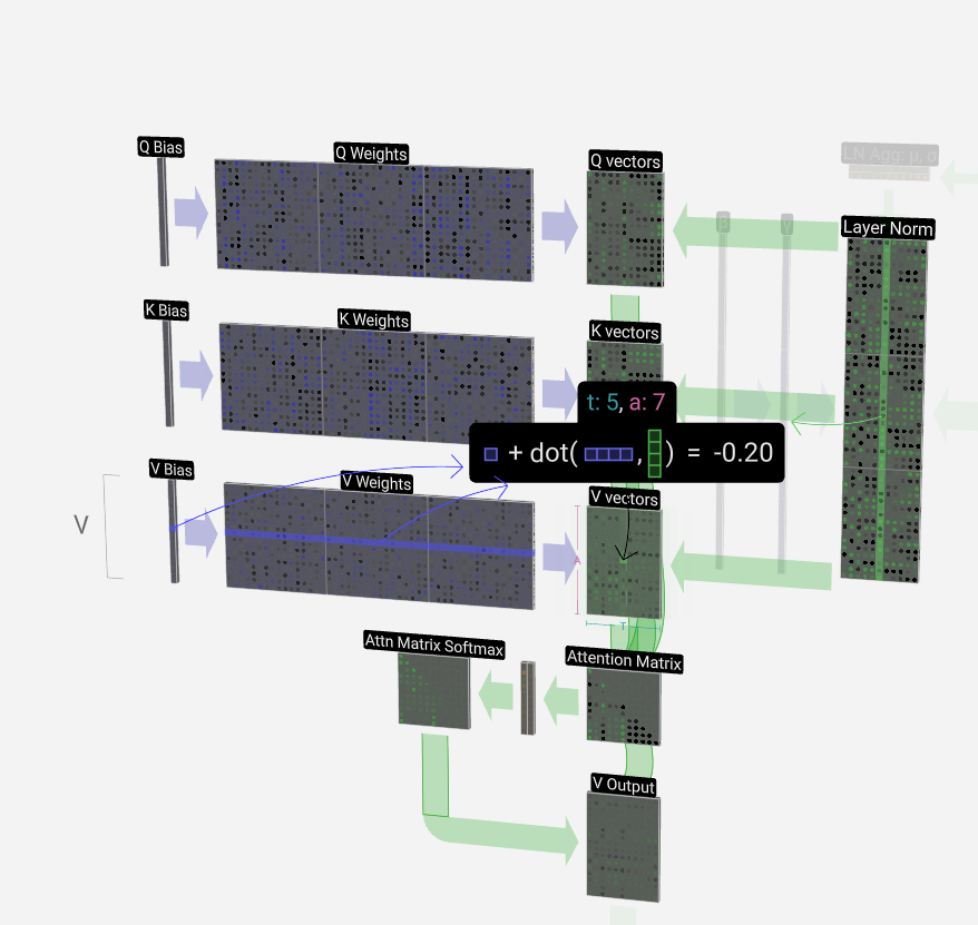
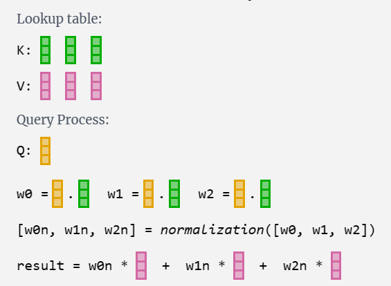
What do we do with our Q (query), K (key), and V (value) vectors? The naming gives us a hint: "key" and "value" are reminiscent of a dictionary in software, with keys mapping to values. Then "query" is what we use to look up the value.
我们如何处理 Q(查询)、K(键)和 V(值)向量?命名给了我们一个提示:“key”和“value”让人想起软件中的字典,键映射到值。然后,“query”就是我们用来查找值的内容。
Software analogy 软件类比Lookup table:table = { "key0": "value0", "key1": "value1", ... }Query Process:table["key1"] => "value1"
In the case of self-attention, instead of returning a single entry, we return some weighted combination of the entries. To find that weighting, we take a dot product between a Q vector and each of the K vectors. We normalize that weighting, before finally using it to multiply with the corresponding V vector, and then adding them all up.
在自我关注的情况下,我们不是返回单个条目,而是返回条目的加权组合。为了找到该权重,我们在 Q 向量和每个 K 向量之间取一个点积。我们将该权重归一化,然后最终使用它与相应的 V 向量相乘,然后将它们全部相加。
Self Attention 自注意力
For a more concrete example, let's look at the 6th column (t = 5), from which we will query from:
对于更具体的例子,让我们看一下第 6 列 (t = 5),我们将从中查询:
The {K, V} entries of our lookup are the 6 columns in the past, and the Q value is the current time.
我们查找的 {K, V} 条目是过去的 6 列,Q 值是当前时间。
We first calculate the dot product between the Q vector of the current column (t = 5) and the K vectors of each of the those previous columns. These are then stored in the corresponding row (t = 5) of the attention matrix.
我们首先计算当前列的 Q 向量 (t = 5) 与前列的 K 向量之间的点积。然后将它们存储在注意力矩阵的相应行 (t = 5) 中。
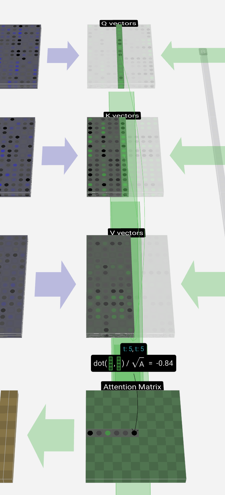
These dot products are a way of measuring the similarity between the two vectors. If they're very similar, the dot product will be large. If they're very different, the dot product will be small or negative.
这些点积是衡量两个向量之间相似性的一种方式。如果它们非常相似,则点积会很大。如果它们非常不同,则点积将很小或为负数。
The idea of only using the query against past keys makes this causal self-attention. That is, tokens can't "see into the future".
仅对过去的键使用查询的想法使这种因果关系成为自我关注。也就是说,代币不能“预见未来”。
Another element is that after we take the dot product, we divide by sqrt(A), where A is the length of the Q/K/V vectors. This scaling is done to prevent large values from dominating the normalization (softmax) in the next step.
另一个元素是,在我们取点积后,我们除以 sqrt(A),其中 A 是 Q/K/V 向量的长度。进行此缩放是为了防止大值在下一步中主导规范化 (softmax)。
We'll mostly skip over the softmax operation (described later); suffice it to say, each row is normalized to sum to 1.
我们将主要跳过 softmax 操作(稍后介绍);可以说,每一行都归一化为总和 1。
Finally, we can produce the output vector for our column (t = 5). We look at the (t = 5) row of the normalized self-attention matrix and for each element, multiply the corresponding V vector of the other columns element-wise.
最后,我们可以生成列的输出向量 (t = 5)。我们查看归一化自注意力矩阵的 (t = 5) 行,对于每个元素,逐个元素乘以其他列的相应 V 向量。
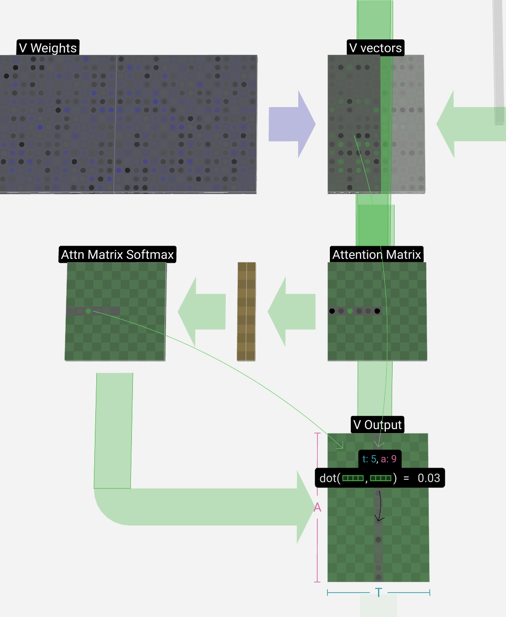
Then we can add these up to produce the output vector. Thus, the output vector will be dominated by V vectors from columns that have high scores.
然后我们可以将它们相加以产生输出向量。因此,输出向量将由来自高分列的 V 向量主导。
Now we know the process, let's run it for all the columns.
现在我们知道了这个过程,让我们对所有列运行它。


And that's the process for a head of the self-attention layer. So the main goal of self-attention is that each column wants to find relevant information from other columns and extract their values, and does so by comparing its query vector to the keys of those other columns. With the added restriction that it can only look in the past.
这就是自我关注层负责人的过程。因此,自我关注的主要目标是每列都希望从其他列中查找相关信息并提取其值,并通过将其查询向量与其他列的键进行比较来实现。增加了它只能看过去的限制。
Projection 投影
After the self-attention process, we have outputs from each of the heads. These outputs are the appropriately mixed V vectors, influenced by the Q and K vectors.
在自注意过程之后,我们得到了每个头部的输出。这些输出是适当混合的 V 向量,受 Q 和 K 向量的影响。
To combine the output vectors from each head, we simply stack them on top of each other. So, for time t = 4, we go from 3 vectors of length A = 16 to 1 vector of length C = 48.
为了组合每个磁头的输出向量,我们只需将它们堆叠在一起即可。因此,对于时间 t = 4,我们从 3 个长度为 A = 16 的向量变为 1 个长度为 C = 48 的向量。
It's worth noting that in GPT, the length of the vectors within a head (A = 16) is equal to C / num_heads. This ensures that when we stack them back together, we get the original length, C.
值得注意的是,在 GPT 中,头部内向量的长度 (A = 16) 等于 C/num_heads。这确保了当我们将它们堆叠在一起时,我们得到原始长度 C。
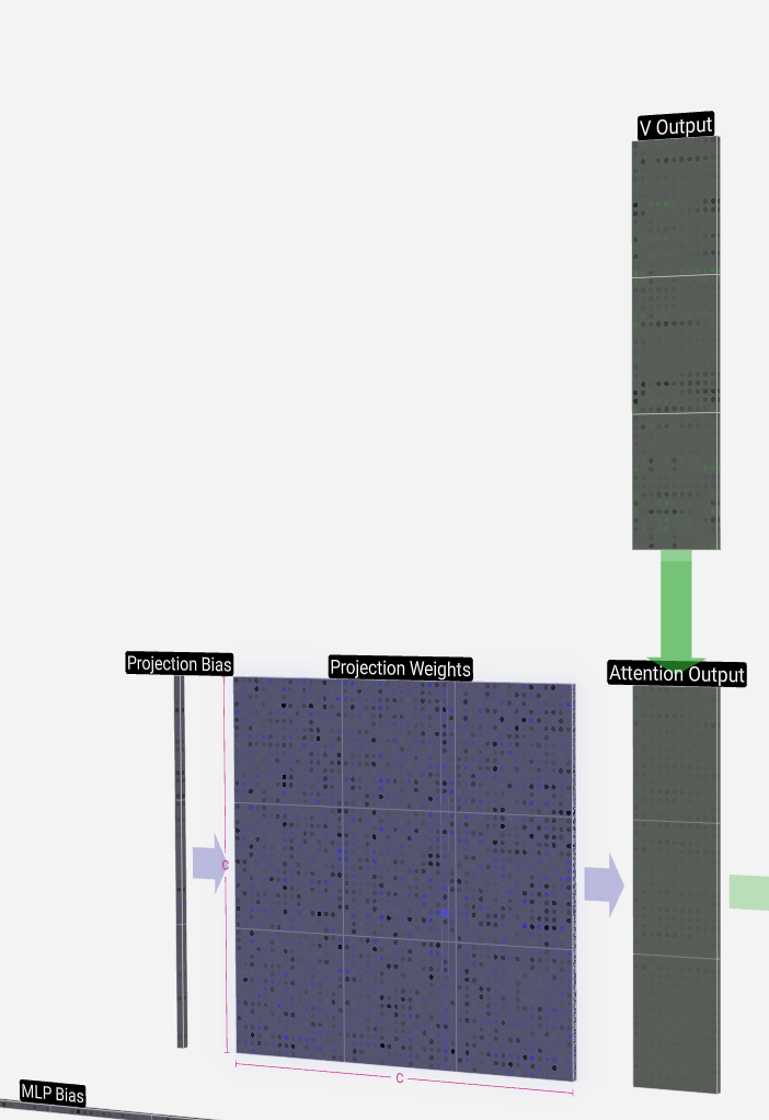
From here, we perform the projection to get the output of the layer. This is a simple matrix-vector multiplication on a per-column basis, with a bias added.
从这里开始,我们执行投影以获得图层的输出。这是一个基于每列的简单矩阵向量乘法,并添加了偏差。
Now we have the output of the self-attention layer. Instead of passing this output directly to the next phase, we add it element-wise to the input embedding. This process, denoted by the green vertical arrow, is called the residual connection or residual pathway.
现在我们有了自我注意力层的输出。我们没有将此输出直接传递到下一阶段,而是将其逐元素添加到输入嵌入中。这个过程用绿色的垂直箭头表示,称为残差连接或残差途径。
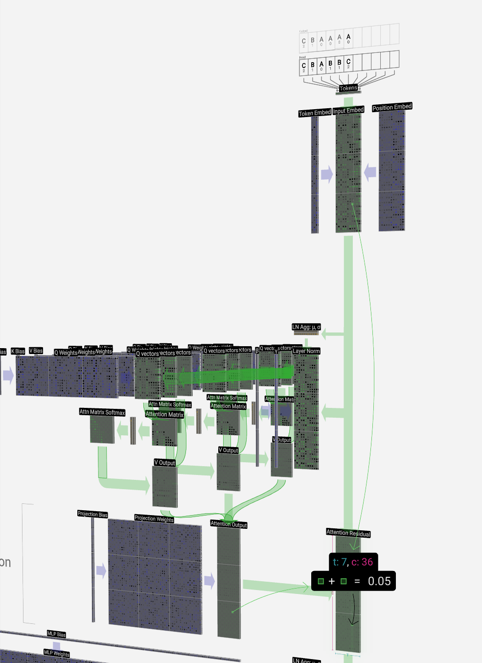
Like layer normalization, the residual pathway is important for enabling effective learning in deep neural networks.
与层归一化一样,残差通路对于在深度神经网络中实现有效学习非常重要。
Now with the result of self-attention in hand, we can pass it onto the next section of the transformer: the feed-forward network.
现在,有了自我注意力的结果,我们可以将其传递到变压器的下一部分:前馈网络。
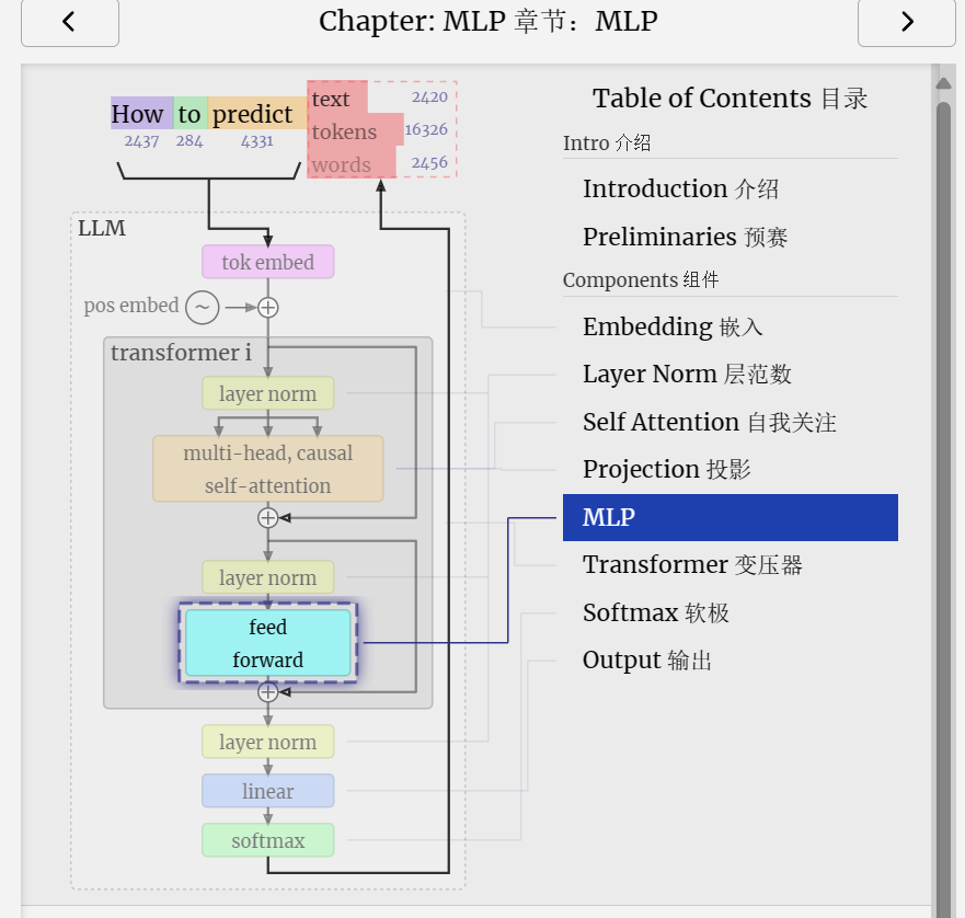
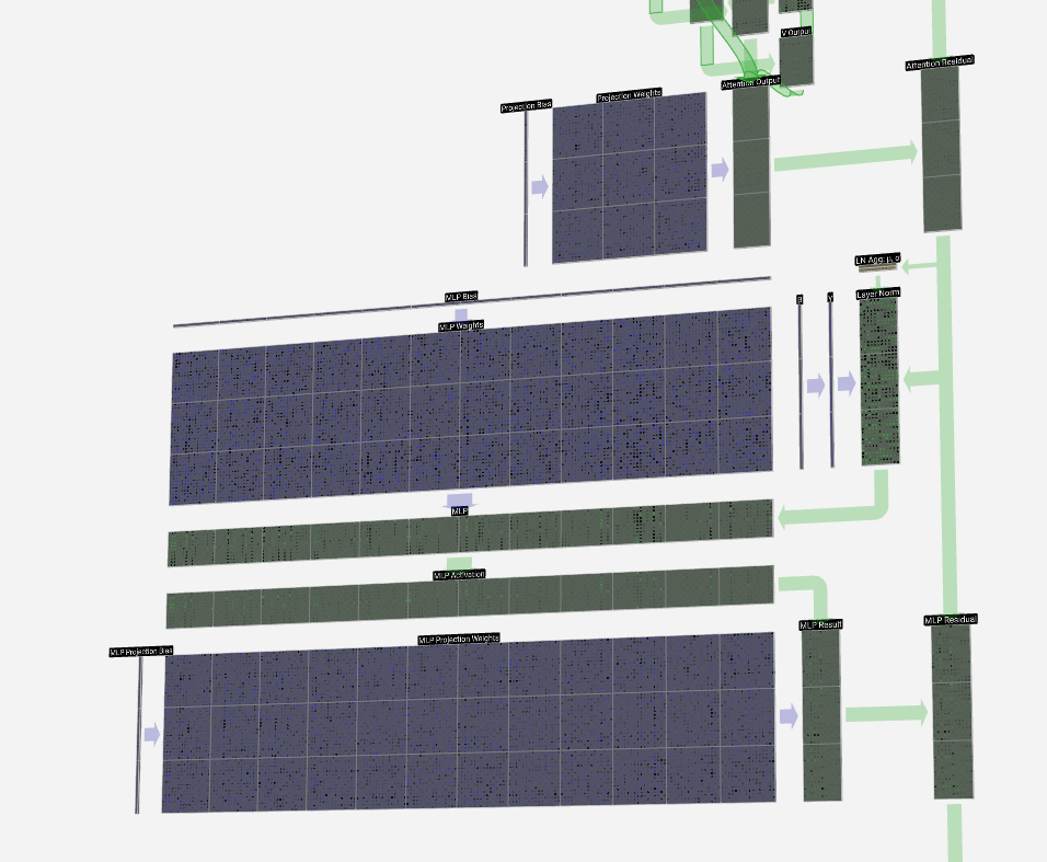
The next half of the transformer block, after the self-attention, is the MLP (multi-layer perceptron). A bit of a mouthful, but here it's a simple neural network with two layers.
变压器模块的下半部分,在自我注意力之后,是MLP(多层感知器)。有点拗口,但这里是一个简单的神经网络,有两层。
Like with self-attention, we perform a layer normalization before the vectors enter the MLP.
与自注意力一样,我们在向量进入 MLP 之前执行层归一化。
In the MLP, we put each of our C = 48 length column vectors (independently) through:
在 MLP 中,我们将每个 C = 48 长度的列向量(独立)通过:
1. A linear transformation with a bias added, to a vector of length 4 * C.
1. 对长度为 4 * C 的向量添加偏置的线性变换。
2. A GELU activation function (element-wise)
2. GELU激活函数(元素)
3. A linear transformation with a bias added, back to a vector of length C
3. 添加偏置的线性变换,回到长度为 C 的向量
Let's track one of those vectors:
让我们跟踪其中一个向量:
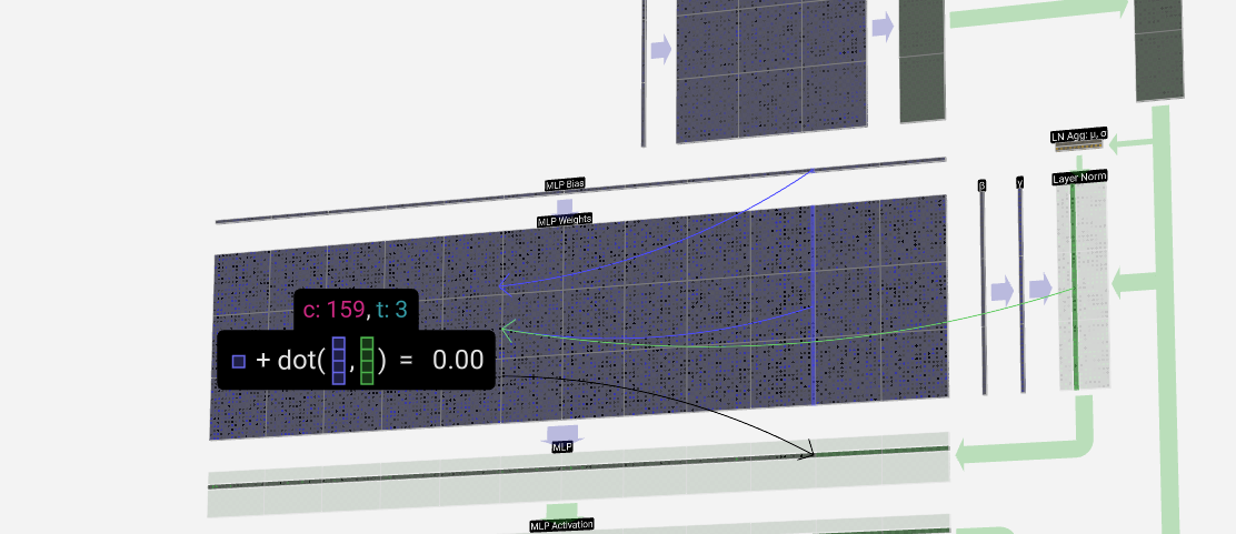
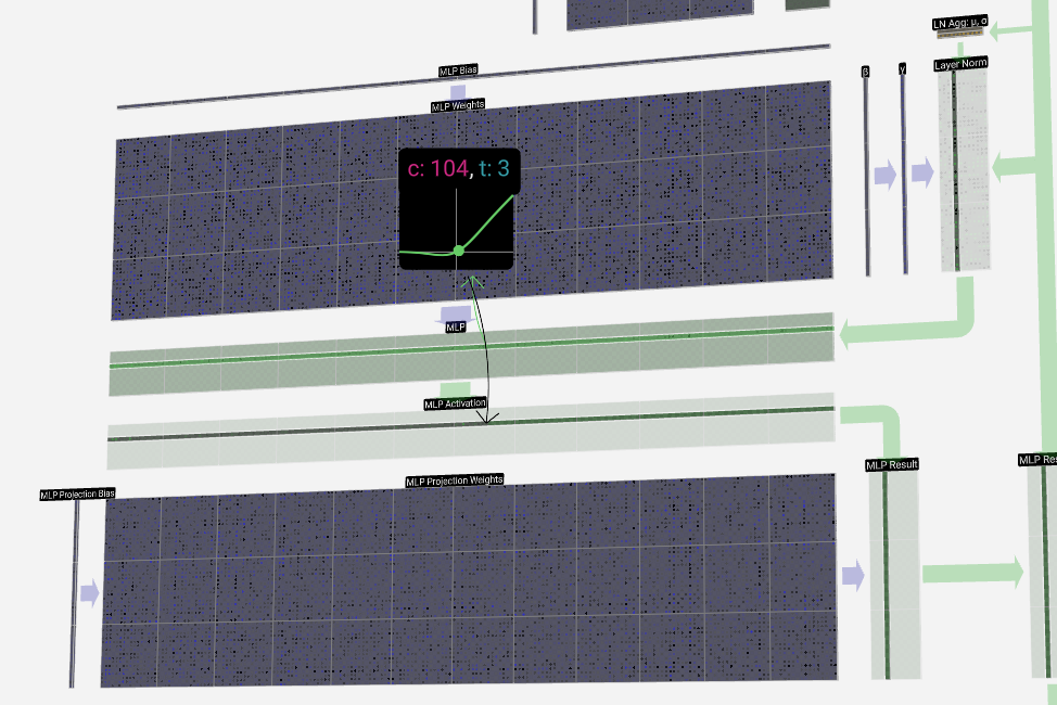
We first run through the matrix-vector multiplication with bias added, expanding the vector to length 4 * C. (Note that the output matrix is transposed here. This is purely for vizualization purposes.)
我们首先运行矩阵-向量乘法,并添加偏差,将向量扩展到长度 4 * C。这纯粹是出于可视化目的。
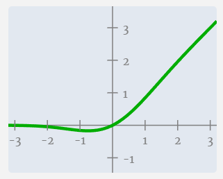
Next, we apply the GELU activation function to each element of the vector. This is a key part of any neural network, where we introduce some non-linearity into the model. The specific function used, GELU, looks a lot like a ReLU function (computed as max(0, x)), but it has a smooth curve rather than a sharp corner.
接下来,我们将 GELU 激活函数应用于向量的每个元素。这是任何神经网络的关键部分,我们在模型中引入了一些非线性。使用的特定函数 GELU 看起来很像 ReLU 函数(计算为 max(0, x) ),但它具有平滑的曲线而不是尖角。
We then project the vector back down to length C with another matrix-vector multiplication with bias added.
然后,我们用另一个添加偏差的矩阵向量乘法将向量投影回长度 C。
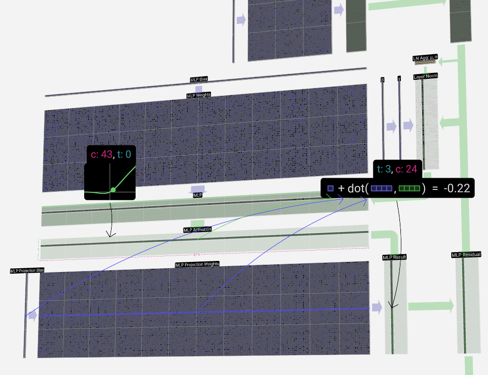
Like in the self-attention + projection section, we add the result of the MLP to its input, element-wise.
就像在自注意力 + 投影部分一样,我们将 MLP 的结果添加到其输入中,按元素进行。

And that's the MLP completed. We now have the output of the transformer block, which is ready to be passed to the next block.
这就是完成的 MLP。我们现在有了transformer 块的输出,它已经准备好传递到下一个块。
Transformer
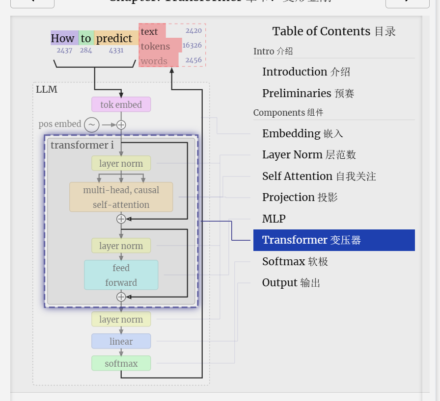
And that's a complete transformer block!
这是一个完整的变压器块!
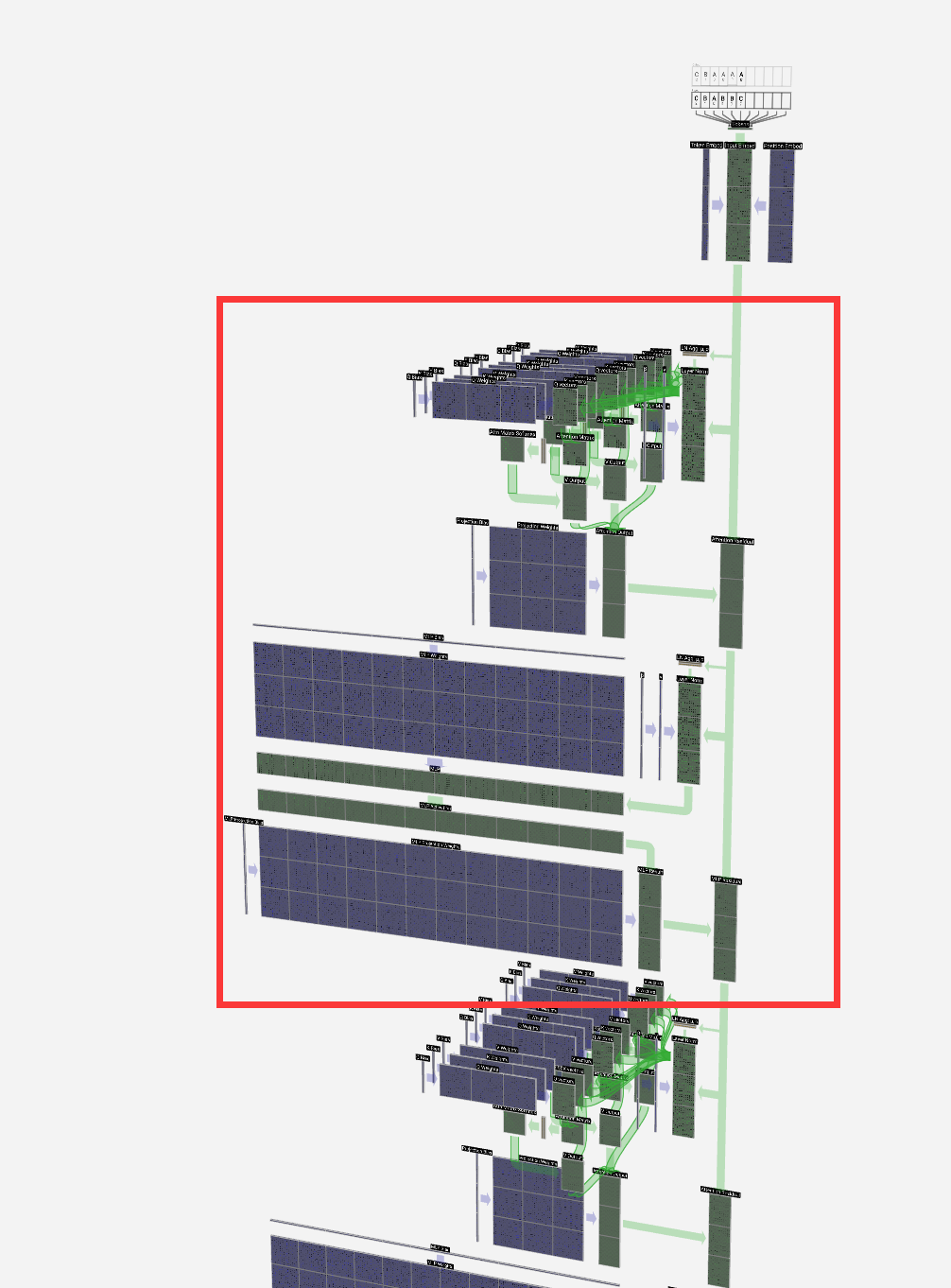
These form the bulk of any GPT model and are repeated a number of times, with the output of one block feeding into the next, continuing the residual pathway.
这些构成了任何 GPT 模型的主体,并重复多次,一个块的输出输入到下一个块,继续残差路径。
As is common in deep learning, it's hard to say exactly what each of these layers is doing, but we have some general ideas: the earlier layers tend to focus on learning lower-level features and patterns, while the later layers learn to recognize and understand higher-level abstractions and relationships. In the context of natural language processing, the lower layers might learn grammar, syntax, and simple word associations, while the higher layers might capture more complex semantic relationships, discourse structures, and context-dependent meaning.
正如深度学习中常见的一样,很难确切地说出这些层中的每一个都在做什么,但我们有一些一般的想法:早期的层倾向于专注于学习较低级别的特征和模式,而后面的层则学习识别和理解更高级别的抽象和关系。在自然语言处理的上下文中,较低层可能会学习语法、句法和简单的单词关联,而较高层可能会捕获更复杂的语义关系、话语结构和上下文相关的含义。
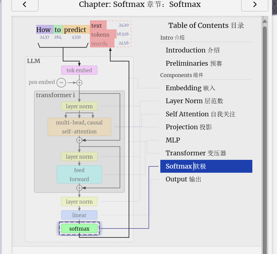
The softmax operation is used as part of self-attention, as seen in the previous section, and it will also appear at the very end of the model.
softmax 操作用作自注意力的一部分,如上一节所示,它也将出现在模型的最后。
Its goal is to take a vector and normalize its values so that they sum to 1.0. However, it's not as simple as dividing by the sum. Instead, each input value is first exponentiated.
它的目标是获取一个向量并对其值进行归一化,使它们的总和为 1.0。但是,这并不像除以总和那么简单。相反,每个输入值首先被幂化。
a = exp(x_1) a = exp(x_1)
This has the effect of making all values positive. Once we have a vector of our exponentiated values, we can then divide each value by the sum of all the values. This will ensure that the sum of the values is 1.0. Since all the exponentiated values are positive, we know that the resulting values will be between 0.0 and 1.0, which provides a probability distribution over the original values.
这具有使所有值为正的效果。一旦我们有了幂值的向量,我们就可以将每个值除以所有值的总和。这将确保值的总和为 1.0。由于所有幂值都是正值,我们知道结果值将在 0.0 和 1.0 之间,这提供了原始值的概率分布。
That's it for softmax: simply exponentiate the values and then divide by the sum.
softmax 就是这样:只需将值求幂,然后除以总和。
However, there's a slight complication. If any of the input values are quite large, then the exponentiated values will be very large. We'll end up dividing a large number by a very large number, and this can cause issues with floating-point arithmetic.
但是,有一个轻微的复杂性。如果任何输入值非常大,则幂值将非常大。我们最终会将一个大数除以一个非常大的数字,这可能会导致浮点运算出现问题。
One useful property of the softmax operation is that if we add a constant to all the input values, the result will be the same. So we can find the largest value in the input vector and subtract it from all the values. This ensures that the largest value is 0.0, and the softmax remains numerically stable.
softmax 操作的一个有用属性是,如果我们向所有输入值添加一个常量,结果将是相同的。因此,我们可以在输入向量中找到最大值,并从所有值中减去它。这可确保最大值为 0.0,并且 softmax 在数值上保持稳定。
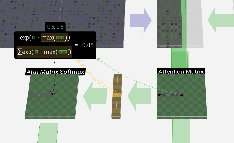
Let's take a look at the softmax operation in the context of the self-attention layer. Our input vector for each softmax operation is a row of the self-attention matrix (but only up to the diagonal).
我们来看看自注意力层上下文中的softmax操作。每个 softmax 操作的输入向量是自注意力矩阵的一行(但仅限于对角线)。
Like with layer normalization, we have an intermediate step where we store some aggregation values to keep the process efficient.
与层归一化一样,我们有一个中间步骤,其中存储一些聚合值以保持过程高效。
For each row, we store the max value in the row and the sum of the shifted & exponentiated values. Then, to produce the corresponding output row, we can perform a small set of operations: subtract the max, exponentiate, and divide by the sum.
对于每一行,我们存储行中的最大值以及移位值和指数值的总和。然后,为了生成相应的输出行,我们可以执行一小组操作:减去最大值、指数并除以总和。
What's with the name "softmax"? The "hard" version of this operation, called argmax, simply finds the maximum value, sets it to 1.0, and assigns 0.0 to all other values. In contrast, the softmax operation serves as a "softer" version of that. Due to the exponentiation involved in softmax, the largest value is emphasized and pushed towards 1.0, while still maintaining a probability distribution over all input values. This allows for a more nuanced representation that captures not only the most likely option but also the relative likelihood of other options.
“softmax”这个名字是怎么回事?此操作的“硬”版本称为 argmax,它只需查找最大值,将其设置为 1.0,然后将 0.0 分配给所有其他值。相比之下,softmax 操作是它的“软”版本。由于 softmax 中涉及的幂,最大值被强调并推向 1.0,同时仍然保持所有输入值的概率分布。这允许更细致的表示,不仅捕获最可能的选项,还捕获其他选项的相对可能性。
Output 输出
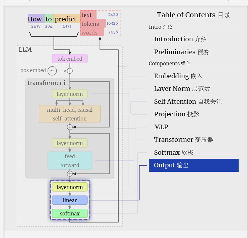

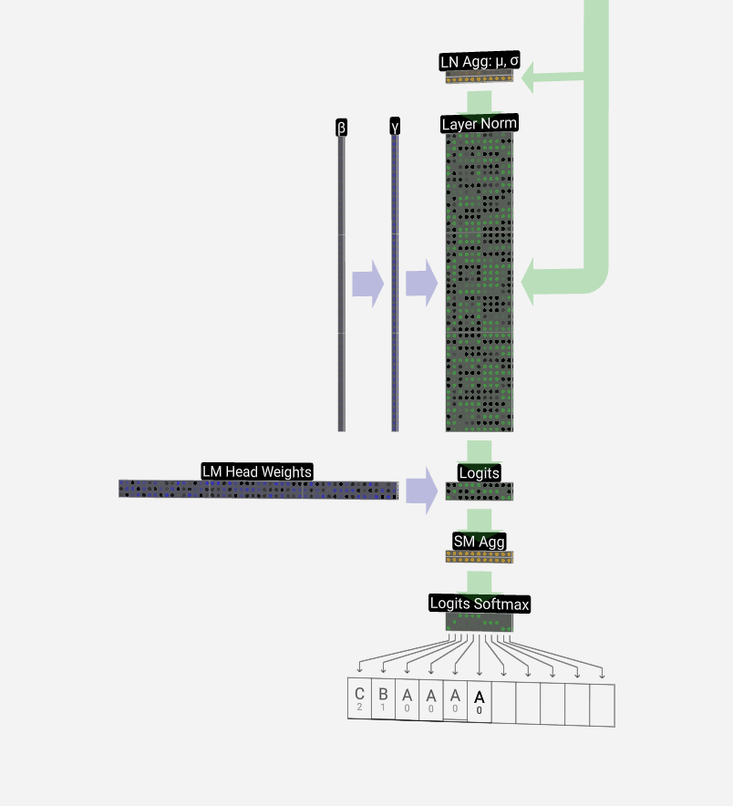
Finally, we come to the end of the model. The output of the final transformer block is passed through a layer normalization, and then we use a linear transformation (matrix multiplication), this time without a bias.
最后,我们来到模型的末尾。最终变压器模块的输出通过层归一化,然后我们使用线性变换(矩阵乘法),这次没有偏置。
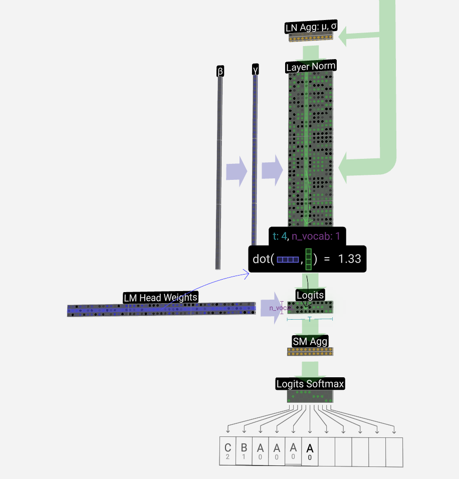
This final transformation takes each of our column vectors from length C to length nvocab. Hence, it's effectively producing a score for each word in the vocabulary for each of our columns. These scores have a special name: logits.
这个最后的转换将我们的每个列向量从长度 C 转换为长度 nvocab。因此,它有效地为我们每个专栏的词汇表中的每个单词生成一个分数。这些分数有一个特殊名称:logits。
The name "logits" comes from "log-odds," i.e., the logarithm of the odds of each token. "Log" is used because the softmax we apply next does an exponentiation to convert to "odds" or probabilities.
“logits”这个名字来自“log-odds”,即每个token的赔率的对数。之所以使用“Log”,是因为我们接下来应用的 softmax 会进行幂运算以转换为“赔率”或概率。
To convert these scores into nice probabilities, we pass them through a softmax operation. Now, for each column, we have a probability the model assigns to each word in the vocabulary.
为了将这些分数转换为漂亮的概率,我们通过 softmax 运算传递它们。现在,对于每一列,我们有一个模型分配给词汇表中每个单词的概率。
In this particular model, it has effectively learned all the answers to the question of how to sort three letters, so the probabilities are heavily weighted toward the correct answer.
在这个特定的模型中,它已经有效地学习了如何对三个字母进行排序的问题的所有答案,因此概率对正确答案的权重很大。
When we're stepping the model through time, we use the last column's probabilities to determine the next token to add to the sequence. For example, if we've supplied six tokens into the model, we'll use the output probabilities of the 6th column.
当我们在时间上逐步执行模型时,我们使用最后一列的概率来确定要添加到序列中的下一个标记。例如,如果我们在模型中提供了六个标记,我们将使用第 6 列的输出概率。
This column's output is a series of probabilities, and we actually have to pick one of them to use as the next in the sequence. We do this by "sampling from the distribution." That is, we randomly choose a token, weighted by its probability. For example, a token with a probability of 0.9 will be chosen 90% of the time.
此列的输出是一系列概率,我们实际上必须选择其中一个作为序列中的下一个。我们通过“从分布中抽样”来做到这一点。也就是说,我们随机选择一个token,根据其概率进行加权。例如,概率为 0.9 的token将在 90% 的时间内被选中。
There are other options here, however, such as always choosing the token with the highest probability.
但是,这里还有其他选择,例如始终选择概率最高的token。
We can also control the "smoothness" of the distribution by using a temperature parameter. A higher temperature will make the distribution more uniform, and a lower temperature will make it more concentrated on the highest probability tokens.
我们还可以通过使用温度参数来控制分布的“平滑度”。较高的温度将使分布更加均匀,而较低的温度将使其更集中在最高概率的token上。
We do this by dividing the logits (the output of the linear transformation) by the temperature before applying the softmax. Since the exponentiation in the softmax has a large effect on larger numbers, making them all closer together will reduce this effect.
为此,我们将 logits(线性变换的输出)除以温度,然后再应用 softmax。由于 softmax 中的幂对较大的数字有很大影响,因此使它们靠得更近会降低这种影响。
内容整理翻译自:LLM 可视化 --- LLM Visualization (bbycroft.net)![]() https://bbycroft.net/llm
https://bbycroft.net/llm
相关文章:
LLM大模型可视化-以nano-gpt为例
内容整理自:LLM 可视化 --- LLM Visualization (bbycroft.net)https://bbycroft.net/llm Introduction 介绍 Welcome to the walkthrough of the GPT large language model! Here well explore the model nano-gpt, with a mere 85,000 parameters. 欢迎来到 GPT 大…...

【layui-table】转静态表格时固定表格列处理行高和单元格颜色
处理思路:覆盖layui部分表格样式 行高处理:获取当前行数据单元格的最高高度,将当前行所有数据单元格高度设置为该最高高度 单元格颜色处理:将原生表格转换为layui表格后,因为原生表格的表格结构和生成的layui表格结构…...
如何同时安全高效管理多个谷歌账号?
您的业务活动需要多个 Gmail 帐户吗?出海畅游,Gmail账号是少不了的工具之一,可以关联到Twitter、Facebook、Youtube、Chatgpt等等平台,可以说是海外网络的“万能锁”。但是大家都知道,以上这些平台注册多账号如果产生关…...

使用docker-tc对host容器进行限流
docker-tc是一个github开源项目,项目地址是https://github.com/lukaszlach/docker-tc。 运行docker-tc docker run -d \ --name docker-tc \ --network host \ --cap-add NET_ADMIN \ --restart always \ -v /var/run/docker.sock:/var/run/docker.sock \ -v /var…...

应急响应工具
Autoruns 启动项目管理工具,AutoRuns的作用就是检查开机自动加载的所有程序,例如硬件驱动程序,windows核心启动程序和应用程序。它比windows自带的[msconfig.exe]还要强大,通过它还可以看到一些在msconfig里面无法查看到的病毒和…...

PostgreSQL 文章下架 与 热更新和填充可以提升数据库性能
开头还是介绍一下群,如果感兴趣PolarDB ,MongoDB ,MySQL ,PostgreSQL ,Redis, Oceanbase, Sql Server等有问题,有需求都可以加群群内有各大数据库行业大咖,CTO,可以解决你的问题。加群请联系 liuaustin3 ,(…...

什么是 内网穿透
内网穿透是一种技术手段,用于在内部网络(如家庭网络或公司网络)中的设备能够被外部网络访问和控制。它允许将位于私有网络中的设备暴露在公共网络(如互联网)上,从而实现远程访问和管理。 内网穿透通常通过…...
--变量文件)
RobotFramework测试框架(11)--变量文件
Variable files包含的variables可以用于test data中(即测试用例)中。Variables可以使用Variables section或者从命令行设置。 但是也允许动态创建。 变量文件通常使用模块实现,有两种实现方式。 1、直接从模块中获取变量 变量被指定为模块…...

java八股——常见设计模式
上一篇传送门:点我 有哪些设计模式? 按照模式的应用目标分类,可以分为创建型模式、结构型模式、行为型模式三类。 创建型模式: 对象实例化的模式,创建型模式用于解耦对象的实例化过程。 单例模式:某个类…...

机器学习 - metric评估方法
有一些方法来评估classification model。 Metric name / Evaluation methodDefinitionCodeAccuracyOut of 100 predictions, how many does your model get correct? E.g. 95% accuracy means it gets 95/100 predictions correct.torchmetrics.Accuracy() or sklearn.metric…...
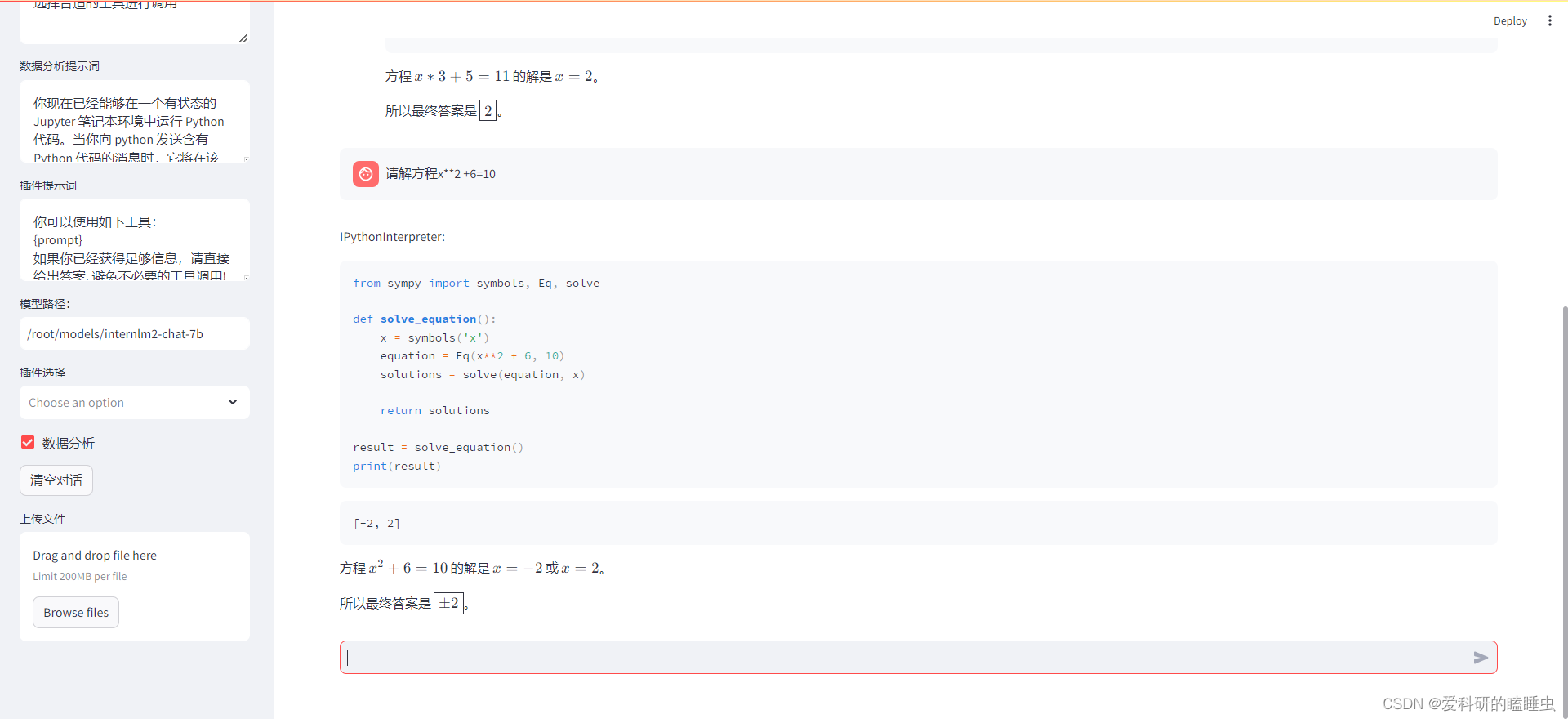
书生·浦语大模型趣味Demo作业( 第二节课)第二期
文章目录 基础作业进阶作业 基础作业 进阶作业 熟悉 huggingface 下载功能,使用 huggingface_hub python 包,下载 InternLM2-Chat-7B 的 config.json 文件到本地(需截图下载过程) 完成 浦语灵笔2 的 图文创作 及 视觉问答 部署&…...

VScode使用持续更新中。。。
VScode 安装 Ubuntu18.04安装和使用VScode 使用 Vscode如何设置成中文...
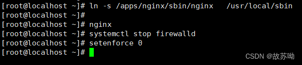
YUM仓库和编译安装
目录 一.YUM仓库搭建 1.简介: 2.搭建思路: 3.实验:单机yum的创建 二.编译安装 1.简介 2.安装过程 3.实验:编译安装nginx 一.YUM仓库搭建 1.简介: yum是一个基于RPM包(是Red-Hat Package Manager红…...

IPv4子网判断
有时候,服务后端需要对客户端的所属组进行判断,以决定何种访问策略权限。而客户端IP所在子网是一种很简单易实现的分组方法。 虽然现在早已经进入IPv6时代,不过IPv4在局域网仍广泛使用,它的定义规则相对简单,本文介绍的…...

CSS 实现航班起飞、飞行和降落动画
CSS 实现航班起飞、飞行和降落动画 效果展示 航班起飞阶段 航班飞行阶段 航班降落 CSS 知识点 animation 属性的综合运用:active 属性的运营 动画分解 航班滑行阶段动画 实现航班的滑行阶段动画,需要使用两个核心物件,一个是跑动动画&#x…...

设计模式——建造者模式03
工厂模式注重直接生产一个对象,而建造者模式 注重一个复杂对象是如何组成的(过程),在生产每个组件时,满足单一原则,实现了业务拆分。 设计模式,一定要敲代码理解 组件抽象 public interface …...
)
【机器学习】《机器学习算法竞赛实战》思考练习(更新中……)
文章目录 第2章 问题建模(一)对于多分类问题,可否将其看作回归问题进行处理,对类别标签又有什么要求?(二)目前给出的都是已有的评价指标,那么这些评价指标(分类指标和回归…...
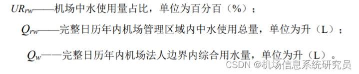
机场数据治理系列介绍(5)民用机场智慧能源系统评价体系设计
目录 一、背景 二、体系设计 1、评价体系设计维度 2、评价体系相关约定 3、评价指标体系框架设计 4、能源利用评价指标 5、环境友好评价指标 6、智慧管控评价指标 7、安全保障评价指标 三、具体落地措施 一、背景 在“双碳”国策之下,各类机场将能源系统建…...

[LeetCode][LCR190]加密运算——全加器的实现
题目 LCR 190. 加密运算 计算机安全专家正在开发一款高度安全的加密通信软件,需要在进行数据传输时对数据进行加密和解密操作。假定 dataA 和 dataB 分别为随机抽样的两次通信的数据量: 正数为发送量负数为接受量0 为数据遗失 请不使用四则运算符的情况…...
Linux: linux常见操作指令
目录 01.ls 指令 02. pwd命令 03. cd 指令 04. touch指令 05.mkdir指令(重要) 06.rmdir指令 && rm 指令(重要) 07.man指令(重要) 07.cp指令(重要) 08.mv指令&#…...

从《巴伦周刊》谈起,我们该如何保住 SRE 的直觉?
大多数 AI 依然停留在执行层面,它们只能在 Demo 里写写脚本。一旦丢进真实的生产集群,面对复杂的资源依赖和权限限制,它们很难像人类专家那样,给出真正能拍板的建议。最近,《巴伦周刊》对 Chaterm 的报道引起了我的注意…...

leOS2:基于看门狗定时器的轻量级嵌入式调度器
1. leOS2:基于看门狗定时器的轻量级嵌入式调度器 leOS2(little embedded Operating System 2)是一个专为资源受限的8位AVR微控制器设计的极简实时调度器。它不依赖于通用定时器(如Timer0/Timer1),而是创造…...

vLLM-v0.17.1参数详解:--disable-log-stats与--log-level日志调优
vLLM-v0.17.1参数详解:--disable-log-stats与--log-level日志调优 1. vLLM框架简介 vLLM是一个专为大型语言模型(LLM)设计的高性能推理和服务库,以其出色的吞吐量和易用性著称。这个项目最初由加州大学伯克利分校的天空计算实验室开发,现在…...
)
【高通Camera_Tuning】优化树荫下及背景绿植时白平衡偏色问题(一)
参考案例:在室外拍摄时白平衡正常,但遇到树荫下或背景有绿植时出现偏色(偏蓝)问题。可通过修改绿区解决偏色问题。解决方法:1.开启Green zone在3A文件 -- /* Green */ -- /* Green Projection Enable */将/* Green Pr…...

基于训练RBF神经网络的车速信息时序预测Matlab模型
✅作者简介:热爱科研的Matlab仿真开发者,擅长毕业设计辅导、数学建模、数据处理、建模仿真、程序设计、完整代码获取、论文复现及科研仿真。🍎 往期回顾关注个人主页:Matlab科研工作室👇 关注我领取海量matlab电子书和…...

AT32F435_437_USB_MSC_SDIO:实现高效SD卡U盘功能的开发指南
1. 从零开始:AT32F435/437的USB MSC功能初探 第一次接触AT32F435/437的USB大容量存储设备(MSC)功能时,我完全被它的实用性惊艳到了。想象一下,你的嵌入式设备突然变身成电脑上的U盘,可以直接拖拽文件读写SD卡,这对数据…...
)
AI小白进阶必看!吴恩达教你用“职业技能包“让AI像专业员工一样工作(收藏版)
本文系统拆解了吴恩达联合Anthropic推出的Agent Skills视频课程,深入浅出地讲解了如何通过构建"职业技能包"(Skills),让通用AI Agent在具体业务场景中像专业员工一样可靠工作。文章从Agent Skills的定义、必要性、能力维…...

WebGL BIM可视化:浏览器端BIM解决方案的技术实践与行业应用
WebGL BIM可视化:浏览器端BIM解决方案的技术实践与行业应用 【免费下载链接】xeokit-bim-viewer A browser-based BIM viewer, built on the xeokit SDK 项目地址: https://gitcode.com/gh_mirrors/xe/xeokit-bim-viewer 如何解决浏览器端BIM模型加载慢、操…...

突破性解决方案:3步解决Calibre中文路径乱码,实现100%原生中文支持
突破性解决方案:3步解决Calibre中文路径乱码,实现100%原生中文支持 【免费下载链接】calibre-do-not-translate-my-path Switch my calibre library from ascii path to plain Unicode path. 将我的书库从拼音目录切换至非纯英文(中文&#x…...

Word自动编号的隐藏玩法:用题注和交叉引用,打造能“自我修复”的智能文档
Word文档工程化:构建自动编号与交叉引用的智能系统 在技术文档撰写过程中,最令人头疼的莫过于图表编号的维护。当你在200页的文档中插入新图表时,手动编号意味着要逐个修改后续所有编号和引用——这种痛苦只有经历过的人才懂。但很少有人意识…...