数据挖掘与分析部分实验与实训项目报告
一、机器学习算法的应用
1. 朴素贝叶斯分类器
相关代码
import pandas as pd
from sklearn.model_selection import train_test_split
from sklearn.naive_bayes import GaussianNB, MultinomialNB
from sklearn.metrics import accuracy_score
# 将数据加载到DataFrame中,删除ID和ZIP Code列
df = pd.read_csv('universalbank.csv')
df = df.drop(columns=['ID', 'ZIP Code'])
# 以下是使用高斯朴素贝叶斯分类器的代码
# 分离特征和目标变量
X = df.drop(columns=['Personal Loan'])
y = df['Personal Loan']
# 划分数据集
# X_train, X_test, y_train, y_test = train_test_split(X, y, test_size=0.3, random_state=42)
X_train, X_test, y_train, y_test = train_test_split(X, y, test_size=0.3, random_state=0)
# 创建高斯朴素贝叶斯分类器实例
gnb = GaussianNB()
# 训练模型
gnb.fit(X_train, y_train)
# 预测测试集
y_pred = gnb.predict(X_test)
# 输出预测结果和模型准确度
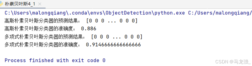
print("高斯朴素贝叶斯分类器的预测结果:", y_pred)
print("高斯朴素贝叶斯分类器的准确度:", accuracy_score(y_test, y_pred))
# 以下是使用多项式朴素贝叶斯分类器的代码
# 筛选出离散型特征
X_discrete = df[['Family', 'Education', 'Securities Account', 'CD Account', 'Online', 'CreditCard']]
# 划分数据集
# X_train_discrete, X_test_discrete, y_train, y_test = train_test_split(X_discrete, y, test_size=0.3, random_state=42)
X_train_discrete, X_test_discrete, y_train, y_test = train_test_split(X_discrete, y, test_size=0.3, random_state=0)
# 创建多项式朴素贝叶斯分类器实例
mnb = MultinomialNB()
# 训练模型
mnb.fit(X_train_discrete, y_train)
# 预测测试集
y_pred_discrete = mnb.predict(X_test_discrete)
# 输出预测结果和模型准确度
print("多项式朴素贝叶斯分类器的预测结果:", y_pred_discrete)
print("多项式朴素贝叶斯分类器的准确度:", accuracy_score(y_test, y_pred_discrete))
运行结果
2.K近邻分类器(KNN)
相关代码
import pandas as pd
from sklearn.model_selection import train_test_split
from sklearn.neighbors import KNeighborsClassifier
from sklearn.metrics import accuracy_score# 将数据加载到DataFrame中,删除ID和ZIP Code列
df = pd.read_csv('universalbank.csv')
df = df.drop(columns=['ID', 'ZIP Code'])
# 分离特征和目标变量
X = df.drop(columns=['Personal Loan'])
y = df['Personal Loan']
# 划分数据集
X_train, X_test, y_train, y_test = train_test_split(X, y, test_size=0.3, random_state=0)
# 创建KNN分类器实例,设置最近邻的数量K为5
knn = KNeighborsClassifier(n_neighbors=5)
# 训练模型
knn.fit(X_train, y_train)
# 预测测试集
y_pred = knn.predict(X_test)
# 输出预测结果和模型准确度
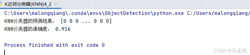
print("KNN分类器的预测结果:", y_pred)
print("KNN分类器的准确度:", accuracy_score(y_test, y_pred))运行结果
3. CART决策树
相关代码
import pandas as pd
from sklearn.model_selection import train_test_split
from sklearn.tree import DecisionTreeClassifier
from sklearn.metrics import accuracy_score
from sklearn.tree import export_graphviz
import graphviz
# 将数据加载到DataFrame中,删除ID和ZIP Code列
df = pd.read_csv('universalbank.csv')
df = df.drop(columns=['ID', 'ZIP Code'])
# 分离特征和目标变量
X = df.drop(columns=['Personal Loan'])
y = df['Personal Loan']
# 划分数据集
X_train, X_test, y_train, y_test = train_test_split(X, y, test_size=0.3, random_state=0)
# 创建CART决策树分类器实例,设置决策树的深度限制为10层
dt = DecisionTreeClassifier(max_depth=10, random_state=42)
# 训练模型
dt.fit(X_train, y_train)
# 预测测试集
y_pred = dt.predict(X_test)
# 输出预测结果和模型准确度
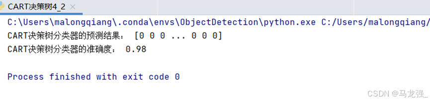
print("CART决策树分类器的预测结果:", y_pred)
print("CART决策树分类器的准确度:", accuracy_score(y_test, y_pred))# 可视化训练好的CART决策树模型
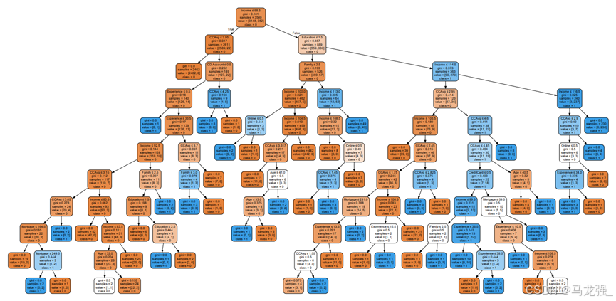
dot_data = export_graphviz(dt, out_file=None,feature_names=X.columns,class_names=['0', '1'],filled=True, rounded=True,special_characters=True)
graph = graphviz.Source(dot_data)
graph.render("universalbank_decision_tree") # 保存为PDF文件
graph.view() # 在默认PDF查看器中打开
运行结果
4.神经网络回归任务
相关代码
import pandas as pd
import numpy as np
from sklearn.model_selection import train_test_split
from sklearn.neural_network import MLPRegressordata = pd.read_csv('house-price.csv')
X = data.iloc[:, 2:14]
y = data.iloc[:, [1]]# 划分数据集,70%为训练集,30%为测试集
X_train, X_test, y_train, y_test = train_test_split(X, y, test_size=0.3, random_state=0)# 创建多层感知机回归模型实例,设置隐藏层层数和神经元数量
regressor = MLPRegressor(hidden_layer_sizes=(100, 10), activation="relu")# 使用训练集数据训练模型
regressor.fit(X_train, y_train)# 使用训练好的模型对测试集进行预测
y_pred = regressor.predict(X_test)# 计算模型的均方误差(MSE)
mse = np.sum(np.square(y_pred - y_test.values)) / len(y_test)
# 计算模型的平均绝对误差(MAE)
mae = np.sum(np.abs(y_pred - y_test.values)) / len(y_test)# 输出测试数据的预测结果和模型的MSE和MAE
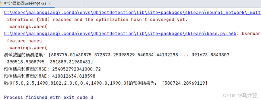
print('测试数据的预测结果:', y_pred)
print("预测结果和模型的MSE:", mse)
print("预测结果和模型的MAE:", mae)
# 使用训练好的模型对给定的数据进行房价预测
y_ = regressor.predict(np.array([[3.0, 2.5, 1490, 8102, 2.0, 0, 0, 4, 1490, 0, 1990, 0]]))
print('数据[3.0,2.5,1490,8102,2.0,0,0,4,1490,0,1990,0]的预测结果为:', y_)运行结果
5.神经网络分类任务
相关代码
import pandas as pd
from sklearn.neural_network import MLPClassifier
from sklearn.metrics import accuracy_score# 将数据加载到DataFrame中
df = pd.read_excel('企业贷款审批数据表.xlsx')
# 选择特征列和目标列
X = df.iloc[:, 1:4] # 特征列X1, X2, X3
y = df.iloc[:, 4] # 目标列Y
# 使用前10行数据作为训练集,11-20行数据作为测试集
X_train = X.iloc[:10]
y_train = y.iloc[:10]
X_test = X.iloc[10:20]
y_test = y.iloc[10:20]
# 创建MLP分类模型实例,设置隐藏层层数和神经元数量
mlp = MLPClassifier(hidden_layer_sizes=(10,5), max_iter=1000, random_state=0,verbose=1)
# 训练模型
mlp.fit(X_train, y_train)
# 使用训练好的模型对测试集进行预测
y_pred = mlp.predict(X_test)
# 计算模型的准确度
accuracy = accuracy_score(y_test, y_pred)
# 输出预测结果和模型准确度
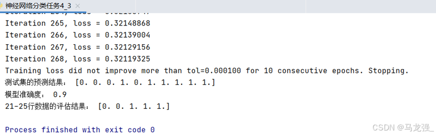
print("测试集的预测结果:", y_pred)
print("模型准确度:", accuracy)
# 使用训练好的模型对21-25行数据进行预测
# 给定的数据
new_data = df.iloc[20:, 1:4]
predicted_results = mlp.predict(new_data)
# 输出评估结果
print("21-25行数据的评估结果:", predicted_results)
运行结果
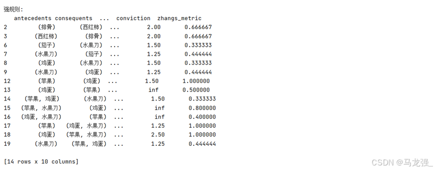
6. 关联规则分析
相关代码
import pandas as pd
from mlxtend.preprocessing import TransactionEncoder
from tabulate import tabulate
from mlxtend.frequent_patterns import apriori, fpgrowth, association_rules# (2)数据读取与预处理
data = pd.read_excel('tr.xlsx', keep_default_na=False)
# 将数据转换为适合TransactionEncoder的格式
te = TransactionEncoder()
te_ary = te.fit(data.values).transform(data.values)
# 创建DataFrame
df = pd.DataFrame(te_ary, columns=te.columns_)
# 剔除第3列到第6列
df = df.drop(columns=df.columns[0:9])
# 将True和False替换为1和0
df = df.replace({True: 1, False: 0})
# 使用tabulate库打印DataFrame
# print(tabulate(df, headers='keys', tablefmt='psql'))# (3)使用apriori算法挖掘频繁项集(最小支持度为0.3)
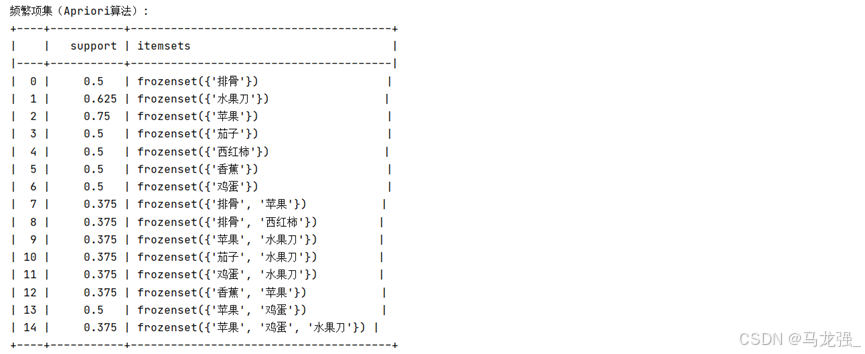
frequent_itemsets_apriori = apriori(df, min_support=0.3, use_colnames=True)# (4)使用FP-growth算法挖掘频繁项集(最小支持度为0.3)
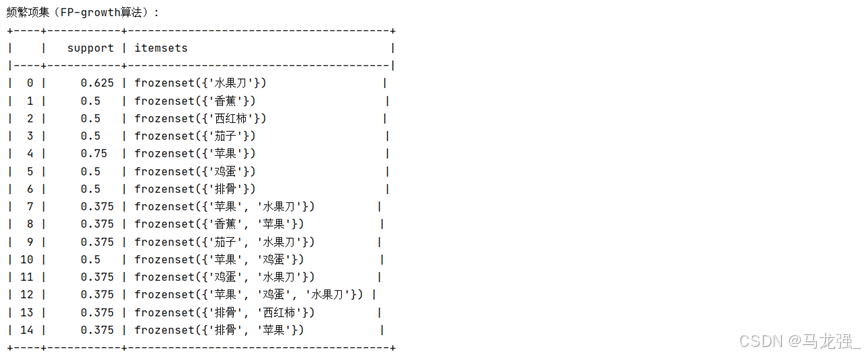
frequent_itemsets_fpgrowth = fpgrowth(df, min_support=0.3, use_colnames=True)# (5)生成强规则(最小置信度为0.5, 提升度>1)
rules = association_rules(frequent_itemsets_apriori, metric='confidence', min_threshold=0.5, support_only=False)
rules = rules[rules['lift'] > 1]# 输出结果
print("频繁项集(Apriori算法):")
# print(frequent_itemsets_apriori)
print(tabulate(frequent_itemsets_apriori, headers='keys', tablefmt='psql'))
print("\n频繁项集(FP-growth算法):")
# print(frequent_itemsets_fpgrowth)
print(tabulate(frequent_itemsets_fpgrowth, headers='keys', tablefmt='psql'))
print("\n强规则:")
print(rules)运行结果
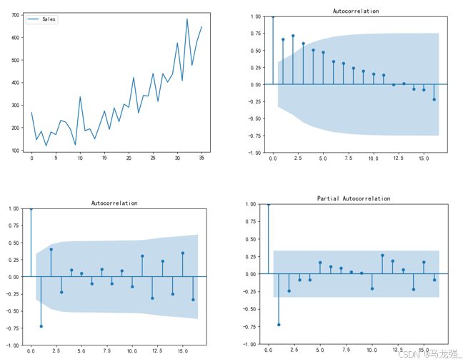
7.时间序列分析
相关代码
import pandas as pd
import warnings
from matplotlib import MatplotlibDeprecationWarning
import matplotlib.pyplot as plt
from statsmodels.graphics.tsaplots import plot_acf, plot_pacf
from statsmodels.tsa.stattools import adfuller as ADF
from statsmodels.tsa.arima.model import ARIMA# 屏蔽所有FutureWarning类型的警告
warnings.filterwarnings("ignore", category=FutureWarning)
warnings.filterwarnings("ignore", category=UserWarning, module="statsmodels")
warnings.filterwarnings("ignore", category=MatplotlibDeprecationWarning)# 读取数据
data = pd.read_csv('shampoo.csv')# 假设数据框中日期列名为'Month'
data['Month'] = '2024-' + data['Month']# 如果需要转换为日期类型(可选)
data['Month'] = pd.to_datetime(data['Month'], format='%Y-%m-%d')
data.rename(columns={'Month': 'Date'}, inplace=True)# (3)检测序列的平稳性
# 时序图判断法
plt.rcParams['font.sans-serif'] = ['SimHei']
plt.rcParams['axes.unicode_minus'] = False
plt.plot(data['Sales'])
plt.legend(['Sales'])
plt.show()# 制自相关图判断法
plot_acf(data['Sales'])
plt.show()# 使用ADF单位根检测法
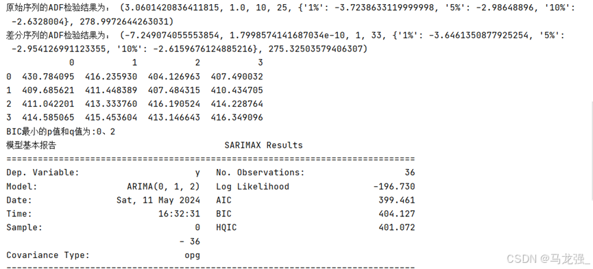
print('原始序列的ADF检验结果为:', ADF(data['Sales']))# (4)差分处理
# 注意:根据上一步结果判断数据序列为非平稳序列,如想使用模型对数据进行建模,
# 则需将数据转换为平稳序列。所以在这一步使用差分处理对序列进行处理。
Date_data = data['Sales'].diff().dropna()# 对处理后的序列进行平稳性检测(自相关图法、偏相关图法、ADF检测法)
plot_acf(Date_data)
plt.show()
plot_pacf(Date_data)
plt.show()print('差分序列的ADF检验结果为:', ADF(Date_data))# (5)使用ARIMA模型对差分处理后的序列进行建模
# 选择合适的p和q值
pmax = int(len(Date_data)/10)
qmax = int(len(Date_data)/10)
bic_matrix = []
for p in range(pmax + 1):tmp = []for q in range(qmax + 1):try:tmp.append(ARIMA(data['Sales'].values, order=(p,1,q)).fit().bic)except:tmp.append(None)bic_matrix.append(tmp)
bic_matrix = pd.DataFrame(bic_matrix)p, q = bic_matrix.stack().idxmin()
print('BIC最小的p值和q值为:%s、%s' % (p, q))# 使用模型预测未来5个月的销售额
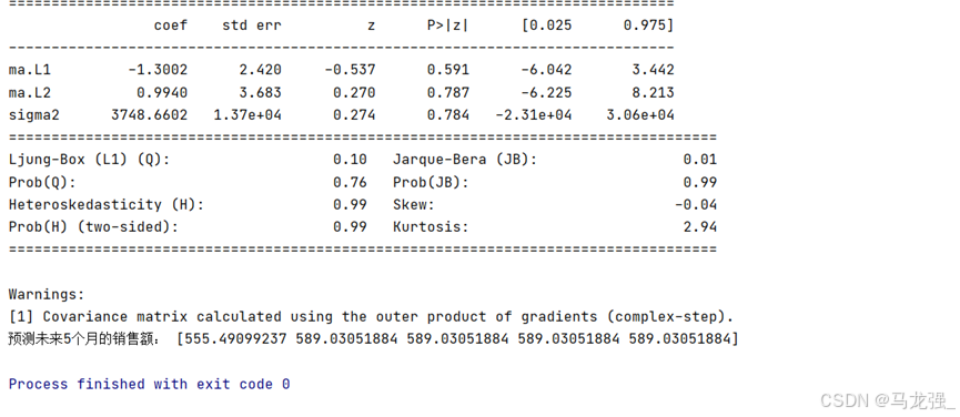
model = ARIMA(data['Sales'].values, order=(p,1,q)).fit()
print('模型基本报告', model.summary())
print('预测未来5个月的销售额:', model.forecast(5))运行结果
二、深度学习算法应用
1. TensorFlow框架的基本使用
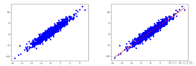
(1)获取训练数据
构建一个简单的线性模型:W,b为参数,W=2,b=1,运用tf.random.normal() 产生1000个随机数,产生x,y数据。
用matplotlib库,用蓝色绘制训练数据。
import tensorflow as tf
import numpy as np
import warnings
from matplotlib import MatplotlibDeprecationWarning# 屏蔽所有FutureWarning类型的警告
warnings.filterwarnings("ignore", category=FutureWarning)
warnings.filterwarnings("ignore", category=UserWarning, module="statsmodels")
warnings.filterwarnings("ignore", category=MatplotlibDeprecationWarning)
W = 3.0   # W参数设置
b =1.0    # b参数设置
num = 1000
# x随机输入
x = tf.random.normal(shape=[num])
# 随机偏差
c = tf.random.normal(shape=[num])
# 构造y数据
y = W * x + b + c
# print(x)# 画图观察
import matplotlib.pyplot as plt    #加载画图库
plt.scatter(x, y, c='b')    # 画离散图
plt.show()    # 展示图
(2)定义模型
通过对样本数据的离散图可以判断,呈线性规律变化,因此可以建立一个线性模型,即 ,把该线性模型定义为一个简单的类,里面封装了变量和计算,变量设置用tf.Variable()。
#定义模型
class LineModel(object):   # 定义一个LineModel的类def __init__(self):# 初始化变量self.W = tf.Variable(5.0)self.b = tf.Variable(0.0)def __call__(self, x):   #定义返回值return self.W * x + self.bdef train(self, x, y, learning_rate):   #定义训练函数with tf.GradientTape() as t:current_loss = loss(self.__call__(x), y)  #损失函数计算# 对W,b求导d_W, d_b = t.gradient(current_loss, [self.W, self.b])# 减去梯度*学习率self.W.assign_sub(d_W*learning_rate)  #减法操作self.b.assign_sub(d_b*learning_rate)
(3)定义损失函数
损失函数是衡量给定输入的模型输出与期望输出的匹配程度,采用均方误差(L2范数损失函数)。
# 定义损失函数
def loss(predicted_y, true_y):   # 定义损失函数return tf.reduce_mean(tf.square(true_y - predicted_y))  # 返回均方误差值
(4)模型训练
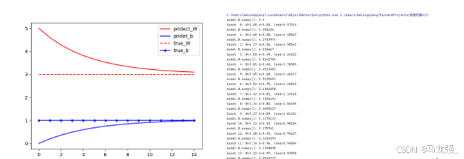
运用数据和模型来训练得到模型的变量(W和b),观察W和b的变化(使用matplotlib绘制W和b的变化情况曲线)。
# 求解过程
model= LineModel()  #运用模型实例化
# 计算W,b参数值的变化
W_s, b_s = [], []    #增加新中间变量
for epoch in range(15):    #循环15次W_s.append(model.W.numpy())  #提取模型的W参数添加到中间变量w_sb_s.append(model.b.numpy())print('model.W.numpy():',model.W.numpy())# 计算损失函数losscurrent_loss = loss(model(x), y)model.train(x, y, learning_rate=0.1)   # 运用定义的train函数训练print('Epoch %2d: W=%1.2f b=%1.2f, loss=%2.5f' %(epoch, W_s[-1], b_s[-1], current_loss))    #输出训练情况
# 画图,把W,b的参数变化情况画出来
epochs = range(15)   #这个迭代数据与上面循环数据一样
plt.figure(1)
plt.scatter(x, y, c='b')    # 画离散图
plt.plot(x,model(x),c='r')
plt.figure(2)
plt.plot(epochs, W_s, 'r',epochs, b_s, 'b')  #画图
plt.plot([W] * len(epochs), 'r--',[b] * len(epochs), 'b-*')
plt.legend(['pridect_W', 'pridet_b', 'true_W', 'true_b'])  # 图例
plt.show()
运行结果
2. 多层神经网络分类
(1)数据获取与预处理
MNIST 数据集来自美国国家标准与技术研究所, National Institute of Standards and Technology (NIST). 训练集 (training set) 由来自 250 个不同人手写的数字构成, 其中 50% 是高中学生, 50% 来自人口普查局 (the Census Bureau) 的工作人员. 测试集(test set) 也是同样比例的手写数字数据。
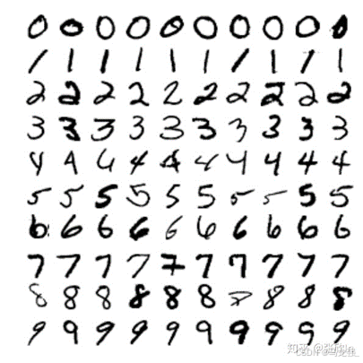
每张图像的大小都是28x28像素。MNIST数据集有60000张图像用于训练和10000张图像用于测试,其中每张图像都被标记了对应的数字(0-9)。
(2)加载数据集
import tensorflow as tf
import matplotlib.pyplot as plt
# 1. 数据获取与预处理
# 加载数据集
mnist = tf.keras.datasets.mnist
(x_train_all, y_train_all), (x_test, y_test) = mnist.load_data()
(3)查看数据集
def show_single_image(img_arr):plt.imshow(img_arr, cmap='binary')plt.show()show_single_image(x_train_all[0])(4)归一化处理
x_train_all, x_test = x_train_all / 255.0, x_test / 255.0模型构建
(5)模型定义
# 模型定义
model = tf.keras.models.Sequential([  #输入层  tf.keras.layers.Flatten(input_shape=(28, 28)),  #隐藏层1  tf.keras.layers.Dense(256, activation=tf.nn.relu),  #百分之20的神经元不工作,防止过拟合  tf.keras.layers.Dropout(0.2),  #隐藏层2  tf.keras.layers.Dense(128, activation=tf.nn.relu),  #隐藏层3  tf.keras.layers.Dense(64, activation=tf.nn.relu),  #输出层  tf.keras.layers.Dense(10, activation=tf.nn.softmax)
])
(6)编译模型
#定义优化器,损失函数,训练效果中计算准确率
model.compile(optimizer='adam', loss='sparse_categorical_crossentropy', metrics=['sparse_categorical_accuracy'])
(7)输出模型参数
# 打印网络参数
print(model.summary())
模型训练
(8)训练
# 训练模型
history = model.fit(x_train_all, y_train_all, epochs=50, validation_split=0.2, verbose=1)
(9)获取训练历史数据中的各指标值
acc = history.history['sparse_categorical_accuracy']
val_acc = history.history['val_sparse_categorical_accuracy']
loss = history.history['loss']
val_loss = history.history['val_loss']
(10)绘制指标在训练过程中的变化图
plt.figure(1)
plt.plot(acc, label='Training Accuracy')
plt.plot(val_acc, label='Validation Accuracy')
plt.title('Training and Validation Accuracy')
plt.legend()
plt.figure(2)
plt.plot(loss, label='Training Loss')
plt.plot(val_loss, label='Validation Loss')
plt.title('Training and Validation Loss')
plt.legend()
plt.show()
(11)模型评估
使用测试集对模型进行评估
loss, accuracy = model.evaluate(x_test, y_test, verbose=1)
print(f"Test Loss: {loss}, Test Accuracy: {accuracy}")
3. 多层神经网络回归
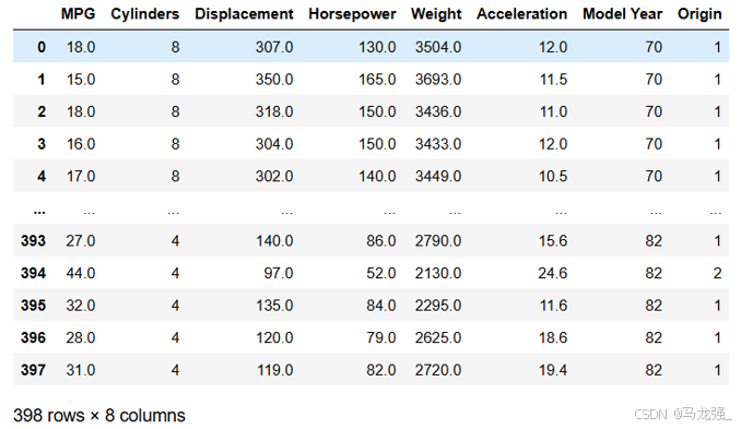
(1)数据获取与预处理
Auto MPG 数据集,它记录了各种汽车效能指标MPG(Mile Per Gallon)与气缸数、重量、马力等因素的真实数据。除了产地的数字字段表示类别外,其他字段都是数值类型。对于产地地段,1 表示美国,2 表示欧洲,3 表示日本。
(2)加载数据集
import pandas as pd
import numpy as np
import seaborn as sns
import matplotlib.pyplot as plt
from sklearn.preprocessing import StandardScaler
from sklearn.model_selection import train_test_split
from tensorflow.keras.models import Sequential
from tensorflow.keras.layers import Dense
column_names = ['MPG', 'Cylinders', 'Displacement', 'Horsepower', 'Weight','Acceleration', 'Model Year', 'Origin']
raw_dataset = pd.read_csv('./data/auto-mpg.data', names=column_names,na_values="?", comment='\t',sep=" ", skipinitialspace=True)
(3)数据清洗
# 数据清洗
# 统计每列的空值数量
null_counts = raw_dataset.isnull().sum()
# 打印每列的空值数量
print(null_counts)
# 删除包含空值的行
dataset = raw_dataset.dropna()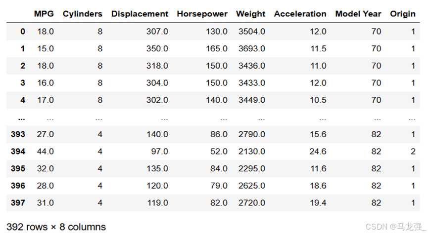
(4)将Origin列转换为one-hot(独热)编码。
dataset = pd.get_dummies(dataset, columns=['Origin'])(5)数据探索
- 使用describe方法查看数据的统计指标
# 使用describe方法查看数据的统计指标
dataset.describe()- 使用seaborn库中pairplot方法绘制"MPG", "Cylinders", "Displacement", "Weight"四列的联合分布图
# 使用seaborn库中pairplot方法绘制"MPG", "Cylinders", "Displacement", "Weight"四列的联合分布图
sns.pairplot(dataset[['MPG', 'Cylinders', 'Displacement', 'Weight']])
(6)数据可视化
labels = dataset.pop('MPG')  #从数据集中取出目标值MPG
#数据标准化
from sklearn.preprocessing import StandardScaler
def norm(x):return (x - train_stats['mean']) / train_stats['std'] #标准化公式
scaler = StandardScaler()
normed_dataset = scaler.fit_transform(dataset)
(7)划分数据集
X_train, X_test, Y_train, Y_test = train_test_split(normed_dataset, labels, test_size=0.2, random_state=0)模型构建
(8)模型定义
import tensorflow as tf
model = tf.keras.Sequential([tf.keras.layers.Dense(64, activation='relu', input_shape=[X_train.shape[1]]),tf.keras.layers.Dense(64, activation='relu'),tf.keras.layers.Dense(1)])
(9)模型编译
model.compile(loss='mse', optimizer='adam', metrics=['mae', 'mse'])
plt.show()
(10)输出模型参数
# 输出模型参数
print(model.summary())
模型训练
(11)训练
history = model.fit(X_train, Y_train, epochs=100, validation_split=0.2, verbose=1)(12)获取训练历史数据中的各指标值
mae = history.history['mae']
val_mae = history.history['val_mae']
mse = history.history['mse']
val_mse = history.history['val_mse']
(13)绘制指标在训练过程中的变化图
plt.figure(figsize=(12, 4))
plt.subplot(1, 2, 1)
plt.plot(mae, label='Training MAE')
plt.plot(val_mae, label='Validation MAE')
plt.title('Training and Validation MAE')
plt.legend()
plt.subplot(1, 2, 2)
plt.plot(mse, label='Training MSE')
plt.plot(val_mse, label='Validation MSE')
plt.title('Training and Validation MSE')
plt.legend()
plt.show()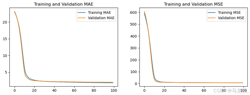
(14)模型评估
使用测试集对模型进行评估
model.evaluate(X_test, Y_test, verbose=1)4. 多层神经网络回归
(1)数据获取与预处理
IMDB数据集,有5万条来自网络电影数据库的评论,其中25000千条用来训练,25000用来测试,每个部分正负评论各占50%。和MNIST数据集类似,IMDB数据集也集成在Keras中,同时经过了预处理:电影评论转换成了一系列数字,每个数字代表字典中的一个单词(表示该单词出现频率的排名)
(2)读取数据
from tensorflow.keras.datasets import imdb
from tensorflow.keras.preprocessing.sequence import pad_sequences
from tensorflow.keras.models import Sequential
from tensorflow.keras.layers import Embedding, LSTM, Dense
from tensorflow.keras.callbacks import EarlyStopping
import tensorflow as tf
# 加载数据,评论文本已转换为整数,其中每个整数表示字典中的特定单词
(x_train, y_train), (x_test, y_test) = imdb.load_data(num_words=10000)
(2)预处理
# 循环神经网络输入长度固定
# 这里应该注意,循环神经网络的输入是固定长度的,否则运行后会出错。
# 由于电影评论的长度必须相同,pad_sequences 函数来标准化评论长度
x_train = tf.keras.preprocessing.sequence.pad_sequences(x_train, maxlen=100)
x_test = tf.keras.preprocessing.sequence.pad_sequences(x_test, maxlen=100)
模型搭建
(3)模型定义
model = Sequential([#定义嵌入层Embedding(10000,  # 词汇表大小中收录单词数量,也就是嵌入层矩阵的行数128,           # 每个单词的维度,也就是嵌入层矩阵的列数input_length=100),# 定义LSTM隐藏层LSTM(128, dropout=0.2, recurrent_dropout=0.2),# 模型输出层Dense(1, activation='sigmoid')
])
(4)编译模型
model.compile(loss='binary_crossentropy',optimizer='adam',metrics=['accuracy'])模型训练
(5)训练
history = model.fit(x_train, y_train, epochs=5, validation_split=0.2, verbose=1)(6)获取训练历史数据中的各指标值
accuracy = history.history['accuracy']
val_accuracy = history.history['val_accuracy']
loss = history.history['loss']
val_loss = history.history['val_loss']
(7)绘制指标在训练过程中的变化图
# 绘制指标在训练过程中的变化图
import matplotlib.pyplot as plt# plt.figure(1)
plt.figure(figsize=(12, 4))
plt.subplot(1, 2, 1)
plt.plot(accuracy, label='Training Accuracy')
plt.plot(val_accuracy, label='Validation Accuracy')
plt.title('Training and Validation Accuracy')
plt.legend()# plt.figure(2)
plt.subplot(1, 2, 2)
plt.plot(loss, label='Training Loss')
plt.plot(val_loss, label='Validation Loss')
plt.title('Training and Validation Loss')
plt.legend()
plt.show()
(8)模型评估
使用测试集对模型进行评估
test_loss, test_acc = model.evaluate(x_test, y_test, verbose=1)
print(f"Test Accuracy: {test_acc}, Test Loss: {test_loss}")
三、数据挖掘综合应用
1.微博评论情感分析
(1)数据读取
新浪微博数据集(网上搜集、作者不详)来源于网上的GitHub社区,有微博10 万多条,都带有情感标注,正负向评论约各 5 万条,用来做情感分析的数据集。
import jieba
import pandas as pd
import re
from wordcloud import WordCloud
import matplotlib.pyplot as plt
from keras.models import Sequential
from keras.layers import Embedding, LSTM, Dense
#from keras.preprocessing.text import Tokenizer
from keras.utils import to_categorical
from sklearn.model_selection import train_test_split
from keras.callbacks import EarlyStoppingdata = pd.read_csv("E:/课程内容文件/大三下学期/数据挖掘与分析/课程实验/实验六/weibo_senti_100.csv")
数据预处理
(2)分词
data['data_cut'] = data['review'].apply(lambda x: jieba.lcut(x))(3)去停用词
with open("E:/课程内容文件/大三下学期/数据挖掘与分析-王思霖/课程实验/实验六/stopword.txt", 'r', encoding='utf-8') as f:stop = f.readlines()
stop = [re.sub('\n', '', r) for r in stop]
data['data_after'] = data['data_cut'].apply(lambda x: [i for i in x if i not in stop and i != '\ufeff'])
(4)词云分析
num_words = [''.join(i) for i in data['data_after']]
num_words = ''.join(num_words)
num = pd.Series(jieba.lcut(num_words)).value_counts()
wc_pic = WordCloud(background_color='white', font_path=r'C:\Windows\Fonts\simhei.ttf').fit_words(num)
plt.figure(figsize=(10, 10))
plt.imshow(wc_pic)
plt.axis('off')
plt.show()
(5)词向量
# 构建词向量矩阵
w = []
for i in data['data_after']:w.extend(i)
# 计算词频
word_counts = pd.Series(w).value_counts()
# 创建DataFrame
num_data = pd.DataFrame(word_counts).reset_index()
# 重命名列
num_data.columns = ['word', 'count']
# 添加id列
num_data['id'] = num_data.index + 1# 创建单词到ID的映射字典
word_to_id_dict = num_data.set_index('word')['id'].to_dict()# 优化的转化成数字函数
def optimized_word2num(x):return [word_to_id_dict[i] for i in x if i in word_to_id_dict]# 应用优化后的函数
data['vec'] = data['data_after'].apply(optimized_word2num)
(6)划分数据集
import tensorflow as tf
# from keras.preprocessing.text import Tokenizer
from tensorflow.keras.preprocessing.sequence import pad_sequencesmaxlen = 128
vec_data = pad_sequences(data['vec'], maxlen=maxlen)
x_train, x_test, y_train, y_test = train_test_split(vec_data, data['label'], test_size=0.2, random_state=0)
模型搭建
(7)模型定义
model = Sequential([Embedding(len(num_data) + 1,  # 词汇表大小中收录单词数量,加1是因为要包括未知词64,  # 每个单词的维度input_length=maxlen),LSTM(64, dropout=0.2, recurrent_dropout=0.2),Dense(1, activation='sigmoid')
])
(8)编译模型
model.compile(loss='binary_crossentropy',optimizer='adam',metrics=['accuracy'])模型训练
(9)训练
history = model.fit(x_train, y_train,epochs=5,validation_split=0.2,verbose=1)
(10)获取训练历史数据中的各指标值
acc = history.history['accuracy']
val_acc = history.history['val_accuracy']
loss = history.history['loss']
val_loss = history.history['val_loss']
(11)绘制指标在训练过程中的变化图
# 绘制训练 & 验证的准确率
plt.figure(figsize=(12, 4))
plt.subplot(1, 2, 1)
plt.plot(acc, label='Training Accuracy')
plt.plot(val_acc, label='Validation Accuracy')
plt.title('Training and Validation Accuracy')
plt.legend()plt.subplot(1, 2, 2)
# 绘制训练 & 验证的损失值
plt.plot(loss, label='Training Loss')
plt.plot(val_loss, label='Validation Loss')
plt.title('Training and Validation Loss')
plt.legend()
plt.show()
(12)模型评估
使用测试集对模型进行评估
score = model.evaluate(x_test, y_test, verbose=0)
print('Test loss:', score[0])
print('Test accuracy:', score[1])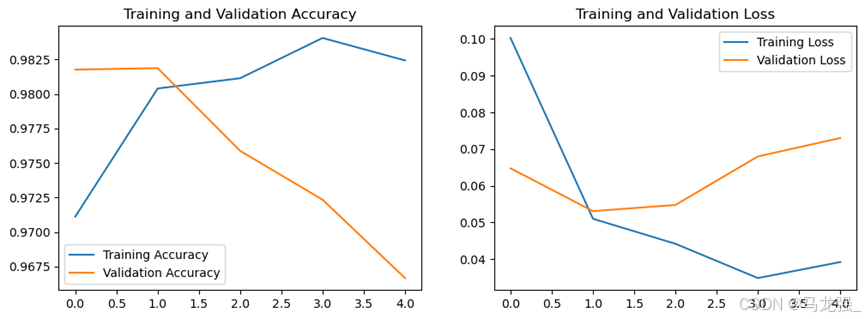
相关文章:
数据挖掘与分析部分实验与实训项目报告
一、机器学习算法的应用 1. 朴素贝叶斯分类器 相关代码 import pandas as pd from sklearn.model_selection import train_test_split from sklearn.naive_bayes import GaussianNB, MultinomialNB from sklearn.metrics import accuracy_score # 将数据加载到DataFrame中&a…...
)
Python中使用SpeechLib实现文本转换语音朗读的示例(修正bug)
一、修正SpeechLib的导入包顺序后的代码: from comtypes.client import CreateObjectengine CreateObject(SAPI.SpVoice) stream CreateObject(SAPI.SpFileStream)from comtypes.gen import SpeechLibinfile E:\\语音文档\\易经64卦读音.txt outfile E:\\demo.…...

政安晨【零基础玩转各类开源AI项目】基于Ubuntu系统部署Hallo :针对肖像图像动画的分层音频驱动视觉合成
政安晨的个人主页:政安晨 欢迎 👍点赞✍评论⭐收藏 收录专栏: 零基础玩转各类开源AI项目 希望政安晨的博客能够对您有所裨益,如有不足之处,欢迎在评论区提出指正! 本文目标:在Ubuntu系统上部署Hallo&#x…...

Spring Boot1(概要 入门 Spring Boot 核心配置 YAML JSR303数据校验 )
目录 一、Spring Boot概要 1. SpringBoot优点 2. SpringBoot缺点 二、Spring Boot入门开发 1. 第一个SpringBoot项目 项目创建方式一:使用 IDEA 直接创建项目 项目创建方式二:使用Spring Initializr 的 Web页面创建项目 (了解&#…...

电脑屏幕录制怎么弄?分享3个简单的电脑录屏方法
在信息爆炸的时代,屏幕上的每一个画面都可能成为我们生活中不可或缺的记忆。作为一名年轻男性,我对于录屏软件的需求可以说是既挑剔又实际。今天,我就为大家分享一下我近期体验的三款录屏软件:福昕录屏大师、转转大师录屏大师和OB…...

idea双击没有反应,打不开
问题描述 Error opening zip file or JAR manifest missing : /home/IntelliJ-IDEA/bin/jetbrains-agent.jar解决方案...

关于UniApp使用的个人笔记
UniApp 开发者中心 用于注册应用以及申请对应证书 https://dev.dcloud.net.cn/pages/app/list https://blog.csdn.net/fred_kang/article/details/124988303 下载证书后,获取SHA1关键cmd keytool -list -v -keystore test.keystore Enter keystore password…...
--perception:object_range_splitter)
autoware.universe源码略读(3.16)--perception:object_range_splitter
autoware.universe源码略读3.16--perception:object_range_splitter Overviewnode(Class Constructor)ObjectRangeSplitterNode::ObjectRangeSplitterNode(mFunc)ObjectRangeSplitterNode::objectCallback Overview 这里处理的依…...

深度学习落地实战:人脸五官定位检测
前言 大家好,我是机长 本专栏将持续收集整理市场上深度学习的相关项目,旨在为准备从事深度学习工作或相关科研活动的伙伴,储备、提升更多的实际开发经验,每个项目实例都可作为实际开发项目写入简历,且都附带完整的代码与数据集。可通过百度云盘进行获取,实现开箱即用 …...

270-VC709E 基于FMC接口的Virtex7 XC7VX690T PCIeX8 接口卡
一、板卡概述 本板卡基于Xilinx公司的FPGA XC7VX690T-FFG1761 芯片,支持PCIeX8、两组 64bit DDR3容量8GByte,HPC的FMC连接器,板卡支持各种FMC子卡扩展。软件支持windows,Linux操作系统。 二、功能和技术指标: 板卡功…...

【go】Excelize处理excel表 带合并单元格、自动换行与固定列宽的文件导出
文章目录 1 简介2 相关需求与实现2.1 导出带单元格合并的excel文件2.2 导出增加自动换行和固定列宽的excel文件 1 简介 之前整理过使用Excelize导出原始excel文件与增加数据校验的excel导出。【go】Excelize处理excel表 带数据校验的文件导出 本文整理使用Excelize导出带单元…...

uniapp自定义tabBar
uniapp自定义tabBar 1、在登录页中获取该用户所有的权限 getAppFrontMenu().then(res>{if(res.length > 0){// 把所有权限存入缓存中let firstPath res.reverse()[0].path;uni.setStorageSync(qx_data, res);uni.switchTab({url: firstPath,})// 方法二 通过uni.setTabB…...

IDEA2023版本创建JavaWeb项目及配置Tomcat详细步骤!
一、创建JavaWeb项目 第一步 之前的版本能够在创建时直接选成Web项目,但是2023版本在创建项目时没有该选项,需要在创建项目之后才能配置,首先先创建一个项目。 第二步 在创建好的项目中选中项目后(一定要注意选中项目名称然后继…...

WPF中MVVM常用的框架
在WPF开发中,MVVM(Model-View-ViewModel)是一种广泛使用的设计模式,它有助于分离应用程序的用户界面(View)、业务逻辑(Model)和数据表现层(ViewModel)。以下是…...

Mysql----内置函数
前言 提示:以下是本篇文章正文内容,下面案例可供参考 一、日期函数 日期:年月日 时间:时分秒 查询:当前时间,只显示当前日期 注意:如果类型为date或者datetime。表中数据类型为date,你插入时…...

去除重复字母
题目链接 去除重复字母 题目描述 注意点 s 由小写英文字母组成1 < s.length < 10^4需保证 返回结果的字典序最小(要求不能打乱其他字符的相对位置) 解答思路 本题与移掉 K 位数字类似,需要注意的是,并不是每个字母都能…...

Xcode进行真机测试时总是断连,如何解决?
嗨。大家好,我是兰若姐姐。最近我在用真机进行app自动化测试的时候,经常会遇到xcode和手机断连,每次断连之后需要重新连接,每次断开都会出现以下截图的报错 当这种情况出现时,之前执行的用例就相当于白执行了ÿ…...

Redis的使用(五)常见使用场景-分布式锁实现原理
1.绪论 为了解决并发问题,我们可以通过加锁的方式来保证数据的一致性,比如java中的synchronize关键字或者ReentrantLock,但是他们只能在同一jvm进程上加锁。现在的项目基本上都是分布式系统,如何对多个java实例进行加锁ÿ…...

AppML 案例:Products
AppML 案例:Products AppML(Application Markup Language)是一种创新的、基于XML的标记语言,旨在简化Web应用程序的开发。它允许开发者通过声明性的方式定义应用程序的界面和数据绑定,从而提高开发效率和减少代码量。…...
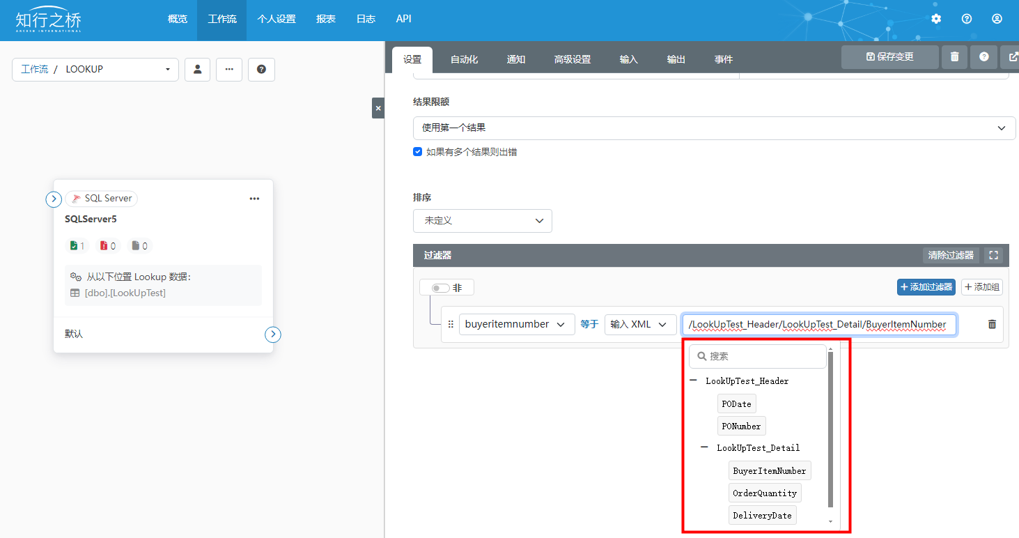
数据库端口LookUp功能:从数据库中获取并添加数据到XML
本文将为大家介绍如何使用知行之桥EDI系统数据库端口的Lookup功能,从数据库中获取数据,并添加进输入的XML中。 使用场景:期待以输入xml中的值为判断条件从数据库中获取数据,并添加进输入xml中。 例如:接收到包含采购…...

新手父母必备:开源婴儿护理知识库架构与核心技能解析
1. 项目概述:一个为新手父母量身定制的技能宝库如果你是一位即将迎来新生命,或者刚刚升级为父母的朋友,面对那个软软糯糯的小家伙,除了满心的喜悦,是不是也时常感到一丝手足无措?喂奶、拍嗝、哄睡、洗澡、抚…...

ClawTick CLI:为AI Agent构建可靠任务调度与监控的实践指南
1. 项目概述:为AI Agent构建可靠的任务调度基础设施 如果你正在开发或使用AI Agent,无论是基于LangChain、CrewAI还是OpenClaw,迟早会遇到一个核心问题:如何让这些智能体定时、可靠地执行任务?自己写个定时脚本&#…...

AI原生Next.js启动器:集成Claude与Cursor的现代前端开发模板
1. 项目概述:一个为AI时代开发者量身定制的Next.js启动器如果你和我一样,每天都在和Next.js、TypeScript、Tailwind CSS打交道,同时又在频繁地与Claude、Cursor、Copilot这些AI编程助手“对话”,那你肯定也遇到过类似的烦恼&#…...

2003年那颗用砂纸磨出来的“中国芯“,毁掉了之后10年国产芯片人的口碑
大家好,我是写代码的篮球球痴。最近这一个多月,我连着写了一串国产芯片创始人——严晓浪、戚肖宁、张建辉、陈志坚、朱一明、王春华。这些人的共同点是:真在干活。有的是熬了20年才把生态做出来,有的是百万年薪不要去创业…...

百度网盘秒传技术:告别重复上传,实现永久分享的终极方案
百度网盘秒传技术:告别重复上传,实现永久分享的终极方案 【免费下载链接】rapid-upload-userscript-doc 秒传链接提取脚本 - 文档&教程 项目地址: https://gitcode.com/gh_mirrors/ra/rapid-upload-userscript-doc 你是否经历过这样的烦恼&am…...

C#循环入门指南:从0到1掌握循环逻辑
一、for循环:已知循环次数,首选它for循环是最常用、最规范的循环,适合已知循环次数的场景(比如打印10遍文字、计算1到100的和)。它的结构很固定,就像一个“固定流程的重复机器”,一步都不会乱。…...
)
告别Excel!用CANalyzer系统变量做CAN信号实时运算,保姆级配置流程(附CAPL脚本)
告别Excel!用CANalyzer系统变量实现CAN信号实时运算的工程实践 在车辆网络数据分析领域,工程师们经常需要验证不同CAN信号之间的理论关系,比如车速与轮速的比例校验、扭矩与电流的线性相关性分析。传统做法是将CANoe/CANalyzer采集的数据导出…...

别再用示波器死磕了!用Python+RC积分电路,5分钟搞定充放电曲线模拟与可视化
别再用示波器死磕了!用PythonRC积分电路,5分钟搞定充放电曲线模拟与可视化 在电子工程实践中,RC积分电路的充放电特性分析是基础中的基础。传统方法往往依赖示波器观测,不仅耗时耗力,还受限于硬件条件。今天ÿ…...
)
毕业设计救星:手把手教你用51单片机和HX711搞定高精度电子秤(附Proteus仿真+完整代码)
毕业设计实战指南:基于51单片机与HX711的高精度电子秤系统开发 在电子信息类专业的毕业设计中,基于51单片机的电子秤系统一直是热门选题。这个项目不仅涵盖了单片机开发的核心技能点,还能让学生深入理解传感器应用、模数转换原理以及人机交互…...

EMC预合规测试:传导与辐射发射的实战指南
1. 预合规EMC测试的核心价值与挑战在电子设备开发领域,电磁兼容性(EMC)问题如同无形的暗礁,往往在产品开发后期才突然显现,导致昂贵的重新设计和上市延迟。我曾参与过一个工业控制设备的项目,团队在功能验证…...