postgresql执行计划解读案例
简介
SQL优化中读懂执行计划尤其重要,以下举例说明在执行计划中常见的参数其所代表的含义。
创建测试数据
-- 创建测试表
drop table if exists customers ;
drop table if exists orders ;
drop table if exists order_items ;
drop table if exists products ;
CREATE TABLE customers (customer_id SERIAL PRIMARY KEY,name VARCHAR(100) NOT NULL,registration_date DATE NOT NULL
);
CREATE TABLE orders (order_id SERIAL PRIMARY KEY,customer_id INT REFERENCES customers(customer_id),order_date DATE NOT NULL,total_amount NUMERIC(10, 2) NOT NULL
);
CREATE TABLE order_items (order_item_id SERIAL PRIMARY KEY,order_id INT REFERENCES orders(order_id),product_name VARCHAR(100) NOT NULL,quantity INT NOT NULL,price_per_item NUMERIC(10, 2) NOT NULL
);
CREATE TABLE products (product_id SERIAL PRIMARY KEY,product_name VARCHAR(100) NOT NULL,product_category VARCHAR(100) NOT NULL,price NUMERIC(10, 2) NOT NULL
);-- 插入数据
INSERT INTO customers (name, registration_date)
VALUES
('Alice', '2022-01-10'),
('Bob', '2022-01-15'),
('Charlie', '2022-01-20');
INSERT INTO products (product_name, product_category, price)
VALUES
('Laptop', 'Electronics', 1200.00),
('Headphones', 'Electronics', 150.00),
('Coffee Maker', 'Home Appliances', 80.00);
INSERT INTO orders (customer_id, order_date, total_amount)
VALUES
(1, '2022-01-12', 1350.00),
(2, '2022-01-16', 80.00),
(3, '2022-01-21', 1200.00);INSERT INTO order_items (order_id, product_name, quantity, price_per_item)
VALUES
(1, 'Laptop', 1, 1200.00),
(1, 'Headphones', 1, 150.00),
(2, 'Coffee Maker', 1, 80.00),
(3, 'Laptop', 1, 1200.00);
创建测试SQL
SELECTc.customer_id,c.name AS customer_name,EXTRACT(YEAR FROM o.order_date) AS order_year,COUNT(o.order_id) AS total_orders,SUM(o.total_amount) AS total_spent,COUNT(oi.order_item_id) AS total_order_items
FROMcustomers c
JOINorders o ON c.customer_id = o.customer_id
JOINorder_items oi ON o.order_id = oi.order_id
GROUP BYc.customer_id, c.name, EXTRACT(YEAR FROM o.order_date)
HAVINGSUM(o.total_amount) > 500
ORDER BYtotal_spent DESC;
可选参数
explain (ANALYZE,BUFFERS,COSTS,FORMAT,GENERIC_PLAN,SETTINGS,SUMMARY,TIMING,VERBOSE,WAL)
ANALYZE:
执行查询并返回实际执行时间和行数统计信息。通过 ANALYZE 参数,您可以得到实际执行的时间、读取的行数以及执行的次数。
BUFFERS:
显示每一步骤的缓冲区(Buffer)访问情况,包括共享缓冲区、临时缓冲区的读取与写入。这能帮助您分析查询是否大量访问磁盘或者是否存在频繁的内存缓冲区使用。
COSTS :
显示估计的执行成本,包括启动成本(执行查询前的初始成本)和总成本。默认情况下,EXPLAIN 会显示成本,使用 COSTS 参数可以控制是否显示这些成本。
FORMAT :
可以指定输出的格式,常用的格式有 JSON TEXT XML YAML 。这对于自动化系统解析查询计划非常有用。
GENERIC_PLAN:
示 EXPLAIN 使用的通用查询计划,而不是为特定参数生成的计划。对于预处理语句或准备好的查询,使用此选项可以查看 PostgreSQL 生成的通用计划。
SETTINGS:
显示在执行查询时使用的设置(如 work_mem、max_parallel_workers_per_gather 等)。这有助于了解查询执行时使用了哪些配置参数。
SUMMARY:
显示执行计划的总结信息,包括计划时间、执行时间、缓冲区统计等。默认情况下,SUMMARY 会显示。
TIMING:
显示每个执行步骤的时间,默认是启用的。禁用后可以减少执行计划输出的细节,这在某些场景下有助于简化分析。
VERBOSE:
显示更多详细信息,包括表名、索引名和每个扫描步骤涉及的列名。适合进行详细调试。
WAL:
显示查询生成了多少 WAL(预写日志)活动。这对于调试写操作尤其有用,可以分析查询对 WAL 的影响。
列举示例
 postgres=# explain (ANALYZE)
postgres-# SELECT
postgres-#     c.customer_id,
postgres-#     c.name AS customer_name,
postgres-#     EXTRACT(YEAR FROM o.order_date) AS order_year,
postgres-#     COUNT(o.order_id) AS total_orders,
postgres-#     SUM(o.total_amount) AS total_spent,
postgres-#     COUNT(oi.order_item_id) AS total_order_items
postgres-# FROM
postgres-#     customers c
postgres-# JOIN
postgres-#     orders o ON c.customer_id = o.customer_id
postgres-# JOIN
postgres-#     order_items oi ON o.order_id = oi.order_id
postgres-# GROUP BY
postgres-#     c.customer_id, c.name, EXTRACT(YEAR FROM o.order_date)
postgres-# HAVING
postgres-#     SUM(o.total_amount) > 500
postgres-# ORDER BY
postgres-#     total_spent DESC;QUERY PLAN
-------------------------------------------------------------------------------------------------------------------------------------Sort  (cost=86.40..86.64 rows=97 width=302) (actual time=0.055..0.057 rows=2 loops=1)Sort Key: (sum(o.total_amount)) DESCSort Method: quicksort  Memory: 25kB->  HashAggregate  (cost=78.61..83.20 rows=97 width=302) (actual time=0.046..0.049 rows=2 loops=1)Group Key: c.customer_id, EXTRACT(year FROM o.order_date)Filter: (sum(o.total_amount) > '500'::numeric)Batches: 1  Memory Usage: 37kBRows Removed by Filter: 1->  Hash Join  (cost=59.83..74.98 rows=290 width=278) (actual time=0.034..0.038 rows=4 loops=1)Hash Cond: (o.customer_id = c.customer_id)->  Hash Join  (cost=42.62..56.29 rows=290 width=32) (actual time=0.014..0.016 rows=4 loops=1)Hash Cond: (oi.order_id = o.order_id)->  Seq Scan on order_items oi  (cost=0.00..12.90 rows=290 width=8) (actual time=0.003..0.004 rows=4 loops=1)->  Hash  (cost=24.50..24.50 rows=1450 width=28) (actual time=0.004..0.005 rows=3 loops=1)Buckets: 2048  Batches: 1  Memory Usage: 17kB->  Seq Scan on orders o  (cost=0.00..24.50 rows=1450 width=28) (actual time=0.003..0.003 rows=3 loops=1)->  Hash  (cost=13.20..13.20 rows=320 width=222) (actual time=0.015..0.015 rows=3 loops=1)Buckets: 1024  Batches: 1  Memory Usage: 9kB->  Seq Scan on customers c  (cost=0.00..13.20 rows=320 width=222) (actual time=0.007..0.008 rows=3 loops=1)Planning Time: 0.301 msExecution Time: 0.097 ms
(21 rows)
以上案例为例,PG执行计划遵循从下到上,从里到外的规则。
-> Hash (cost=24.50..24.50 rows=1450 width=28) (actual time=0.004..0.005 rows=3 loops=1)Buckets: 2048 Batches: 1 Memory Usage: 17kB-> Seq Scan on orders o (cost=0.00..24.50 rows=1450 width=28) (actual time=0.003..0.003 rows=3 loops=1)Seq Scan on orders 对表orders顺序扫描,
(cost=0.00…24.50 rows=1450 width=28) 预估耗费成本,rows=1450预估扫描行1450 width=28预估扫描每行的宽度(以字节为单位),即每行大约占用 28字节。
(actual time=0.003…0.003 rows=3 loops=1) 实际消费成本,0.003…0.003: 0.003排序开始时间,0.003排序结束时间
对orders表扫描结束之后,会对其进行构建hash,常被用关联、嵌套等情况。
(cost=24.50…24.50 rows=1450 width=28) (actual time=0.004…0.005 rows=3 loops=1) 这两段解释同上相同
Buckets: 2048 Batches: 1 Memory Usage: 17kB
Buckets: 2048 表示哈希表中有 2048 个桶,每个桶用于存储散列结果相同的行。这是哈希表的一部分设计,用于分配空间。
Batches: 1 表示只需一批数据处理,因为表的大小足够小,整个哈希表可以存储在内存中。如果数据量非常大,PostgreSQL 可能会将哈希表分成多个批次处理,以防止内存不足。
Memory Usage: 17kB 是哈希表在内存中的大小,显示这次哈希操作所消耗的内存为 17KB。
-> Hash (cost=13.20..13.20 rows=320 width=222) (actual time=0.015..0.015 rows=3 loops=1)Buckets: 1024 Batches: 1 Memory Usage: 9kB-> Seq Scan on customers c (cost=0.00..13.20 rows=320 width=222) (actual time=0.007..0.008 rows=3 loops=1)
Seq Scan on customers c 对customers 表进行顺序扫描, (cost=0.00…13.20 rows=320 width=222)
cost=0.00…13.20 扫描耗费的成本
rows=320 这是估计需要排序的行数
width=222:这是估算每行的宽度(以字节为单位),即每行大约占用 222字节。
actual time=0.007…0.008 为实际耗时,0.007毫秒是排序开始的时间,0.008毫秒是排序结束的时间。
rows=3 表示查询实际排序的行数是 2 行。
loops=1 表示实际执行了一次
Sort (cost=86.40..86.64 rows=97 width=302) (actual time=0.055..0.057 rows=2 loops=1)Sort Key: (sum(o.total_amount)) DESCSort Method: quicksort Memory: 25kB-> HashAggregate (cost=78.61..83.20 rows=97 width=302) (actual time=0.046..0.049 rows=2 loops=1)Group Key: c.customer_id, EXTRACT(year FROM o.order_date)Filter: (sum(o.total_amount) > '500'::numeric)Batches: 1 Memory Usage: 37kBRows Removed by Filter: 1HashAggregate (cost=78.61…83.20 rows=97 width=302) (actual time=0.046…0.049 rows=2 loops=1)
表示进行聚合操作所需要的耗费。
Group Key: c.customer_id, EXTRACT(year FROM o.order_date)
Group Key 表示使用的分组键
Filter: (sum(o.total_amount) > ‘500’::numeric) 表示用的过滤条件
Batches: 1 Memory Usage: 37kB 表示哈希聚合操作占用了 37kB 内存
Rows Removed by Filter: 1 被过滤掉的数据行数
此执行计划可以看出其预估行rows 和实际的rows 有较大的出入。实际上统计信息不是最新信息的问题导致,重新对其analyze单独执行重新收集一下统计信息就可以。
当执行vacuum full之后(也会自动进行analyze)
postgres=# explain (ANALYZE)
postgres-# SELECT
postgres-# c.customer_id,
postgres-# c.name AS customer_name,
postgres-# EXTRACT(YEAR FROM o.order_date) AS order_year,
postgres-# COUNT(o.order_id) AS total_orders,
postgres-# SUM(o.total_amount) AS total_spent,
postgres-# COUNT(oi.order_item_id) AS total_order_items
postgres-# FROM
postgres-# customers c
postgres-# JOIN
postgres-# orders o ON c.customer_id = o.customer_id
postgres-# JOIN
postgres-# order_items oi ON o.order_id = oi.order_id
postgres-# GROUP BY
postgres-# c.customer_id, c.name, EXTRACT(YEAR FROM o.order_date)
postgres-# HAVING
postgres-# SUM(o.total_amount) > 500
postgres-# ORDER BY
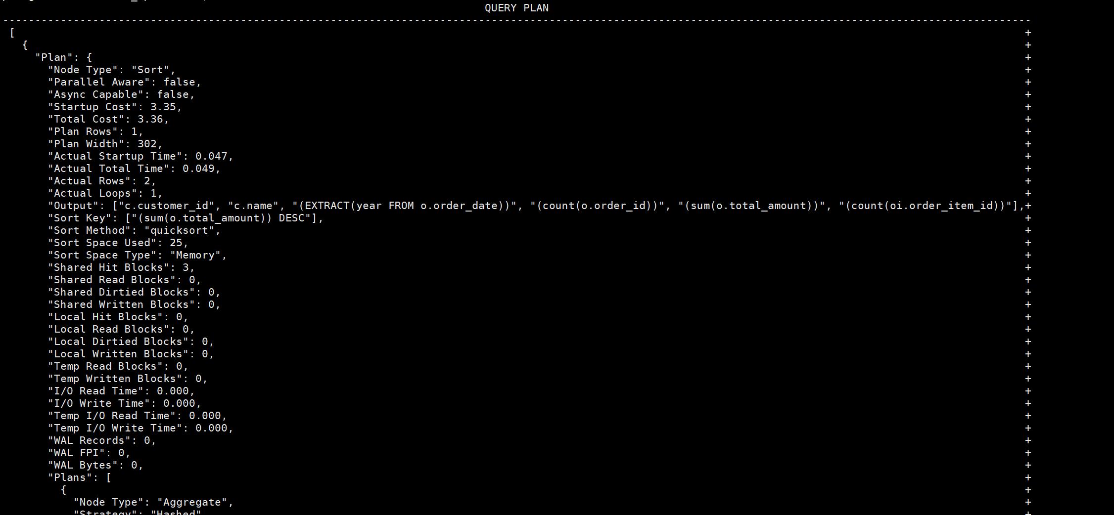
postgres-# total_spent DESC;QUERY PLAN
---------------------------------------------------------------------------------------------------------------------------------Sort (cost=3.35..3.36 rows=1 width=302) (actual time=0.063..0.065 rows=2 loops=1)Sort Key: (sum(o.total_amount)) DESCSort Method: quicksort Memory: 25kB-> HashAggregate (cost=3.28..3.34 rows=1 width=302) (actual time=0.052..0.055 rows=2 loops=1)Group Key: c.customer_id, EXTRACT(year FROM o.order_date)Filter: (sum(o.total_amount) > '500'::numeric)Batches: 1 Memory Usage: 24kBRows Removed by Filter: 1-> Hash Join (cost=2.14..3.23 rows=4 width=278) (actual time=0.037..0.041 rows=4 loops=1)Hash Cond: (o.customer_id = c.customer_id)-> Hash Join (cost=1.07..2.13 rows=4 width=32) (actual time=0.014..0.016 rows=4 loops=1)Hash Cond: (oi.order_id = o.order_id)-> Seq Scan on order_items oi (cost=0.00..1.04 rows=4 width=8) (actual time=0.002..0.003 rows=4 loops=1)-> Hash (cost=1.03..1.03 rows=3 width=28) (actual time=0.005..0.005 rows=3 loops=1)Buckets: 1024 Batches: 1 Memory Usage: 9kB-> Seq Scan on orders o (cost=0.00..1.03 rows=3 width=28) (actual time=0.003..0.004 rows=3 loops=1)-> Hash (cost=1.03..1.03 rows=3 width=222) (actual time=0.014..0.014 rows=3 loops=1)Buckets: 1024 Batches: 1 Memory Usage: 9kB-> Seq Scan on customers c (cost=0.00..1.03 rows=3 width=222) (actual time=0.010..0.010 rows=3 loops=1)Planning Time: 0.568 msExecution Time: 0.129 ms
(21 rows)增加buffers参数之后的执行计划,会增加Buffers: shared hit=3 ,用于记录SQL在执行数据存取过程中使用到了多少个数据块
postgres=# explain (ANALYZE,BUFFERS)
postgres-# SELECT
postgres-#     c.customer_id,
postgres-#     c.name AS customer_name,
postgres-#     EXTRACT(YEAR FROM o.order_date) AS order_year,
postgres-#     COUNT(o.order_id) AS total_orders,
postgres-#     SUM(o.total_amount) AS total_spent,
postgres-#     COUNT(oi.order_item_id) AS total_order_items
postgres-# FROM
postgres-#     customers c
postgres-# JOIN
postgres-#     orders o ON c.customer_id = o.customer_id
postgres-# JOIN
postgres-#     order_items oi ON o.order_id = oi.order_id
postgres-# GROUP BY
postgres-#     c.customer_id, c.name, EXTRACT(YEAR FROM o.order_date)
postgres-# HAVING
postgres-#     SUM(o.total_amount) > 500
postgres-# ORDER BY
postgres-#     total_spent DESC;QUERY PLAN
---------------------------------------------------------------------------------------------------------------------------------Sort  (cost=3.35..3.36 rows=1 width=302) (actual time=0.072..0.074 rows=2 loops=1)Sort Key: (sum(o.total_amount)) DESCSort Method: quicksort  Memory: 25kBBuffers: shared hit=3->  HashAggregate  (cost=3.28..3.34 rows=1 width=302) (actual time=0.053..0.056 rows=2 loops=1)Group Key: c.customer_id, EXTRACT(year FROM o.order_date)Filter: (sum(o.total_amount) > '500'::numeric)Batches: 1  Memory Usage: 24kBRows Removed by Filter: 1Buffers: shared hit=3->  Hash Join  (cost=2.14..3.23 rows=4 width=278) (actual time=0.038..0.043 rows=4 loops=1)Hash Cond: (o.customer_id = c.customer_id)Buffers: shared hit=3->  Hash Join  (cost=1.07..2.13 rows=4 width=32) (actual time=0.013..0.016 rows=4 loops=1)Hash Cond: (oi.order_id = o.order_id)Buffers: shared hit=2->  Seq Scan on order_items oi  (cost=0.00..1.04 rows=4 width=8) (actual time=0.003..0.004 rows=4 loops=1)Buffers: shared hit=1->  Hash  (cost=1.03..1.03 rows=3 width=28) (actual time=0.005..0.005 rows=3 loops=1)Buckets: 1024  Batches: 1  Memory Usage: 9kBBuffers: shared hit=1->  Seq Scan on orders o  (cost=0.00..1.03 rows=3 width=28) (actual time=0.003..0.004 rows=3 loops=1)Buffers: shared hit=1->  Hash  (cost=1.03..1.03 rows=3 width=222) (actual time=0.013..0.014 rows=3 loops=1)Buckets: 1024  Batches: 1  Memory Usage: 9kBBuffers: shared hit=1->  Seq Scan on customers c  (cost=0.00..1.03 rows=3 width=222) (actual time=0.009..0.010 rows=3 loops=1)Buffers: shared hit=1Planning:Buffers: shared hit=2Planning Time: 0.247 msExecution Time: 0.124 ms
增加COSTS参数之后的执行计划中增加了 I/O Timings: shared read 用于解释将数据读取缓存到缓存所需要的时间耗费
Sort (cost=3.35..3.36 rows=1 width=302) (actual time=0.057..0.059 rows=2 loops=1)Sort Key: (sum(o.total_amount)) DESCSort Method: quicksort Memory: 25kBBuffers: shared hit=3-> HashAggregate (cost=3.28..3.34 rows=1 width=302) (actual time=0.049..0.051 rows=2 loops=1)Group Key: c.customer_id, EXTRACT(year FROM o.order_date)Filter: (sum(o.total_amount) > '500'::numeric)Batches: 1 Memory Usage: 24kBRows Removed by Filter: 1Buffers: shared hit=3-> Hash Join (cost=2.14..3.23 rows=4 width=278) (actual time=0.036..0.041 rows=4 loops=1)Hash Cond: (o.customer_id = c.customer_id)Buffers: shared hit=3-> Hash Join (cost=1.07..2.13 rows=4 width=32) (actual time=0.018..0.021 rows=4 loops=1)Hash Cond: (oi.order_id = o.order_id)Buffers: shared hit=2-> Seq Scan on order_items oi (cost=0.00..1.04 rows=4 width=8) (actual time=0.002..0.003 rows=4 loops=1)Buffers: shared hit=1-> Hash (cost=1.03..1.03 rows=3 width=28) (actual time=0.004..0.004 rows=3 loops=1)Buckets: 1024 Batches: 1 Memory Usage: 9kBBuffers: shared hit=1-> Seq Scan on orders o (cost=0.00..1.03 rows=3 width=28) (actual time=0.002..0.003 rows=3 loops=1)Buffers: shared hit=1-> Hash (cost=1.03..1.03 rows=3 width=222) (actual time=0.011..0.011 rows=3 loops=1)Buckets: 1024 Batches: 1 Memory Usage: 9kBBuffers: shared hit=1-> Seq Scan on customers c (cost=0.00..1.03 rows=3 width=222) (actual time=0.007..0.008 rows=3 loops=1)Buffers: shared hit=1Planning:Buffers: shared hit=43 read=3I/O Timings: shared read=0.035Planning Time: 0.432 msExecution Time: 0.114 msI/O Timings: shared read=0.035 表示查询过程中,从磁盘读取到共享缓冲区的数据块总耗时为 0.035 毫秒。这个时间量通常是从物理磁盘读取数据的花费。I/O 时间越短,说明磁盘 I/O 性能越好。
增加FORMAT 修改执行计划输出格式为json格式
explain (ANALYZE,BUFFERS,COSTS,VERBOSE,WAL,FORMAT JSON)SELECTc.customer_id,c.name AS customer_name,EXTRACT(YEAR FROM o.order_date) AS order_year,COUNT(o.order_id) AS total_orders,SUM(o.total_amount) AS total_spent,COUNT(oi.order_item_id) AS total_order_items
FROMcustomers c
JOINorders o ON c.customer_id = o.customer_id
JOINorder_items oi ON o.order_id = oi.order_id
GROUP BYc.customer_id, c.name, EXTRACT(YEAR FROM o.order_date)
HAVINGSUM(o.total_amount) > 500
ORDER BYtotal_spent DESC;
相关文章:
postgresql执行计划解读案例
简介 SQL优化中读懂执行计划尤其重要,以下举例说明在执行计划中常见的参数其所代表的含义。 创建测试数据 -- 创建测试表 drop table if exists customers ; drop table if exists orders ; drop table if exists order_items ; drop table if exists products ;…...
Matlab实现粒子群优化算法优化随机森林算法模型 (PSO-RF)(附源码)
目录 1.内容介绍 2.部分代码 3.实验结果 4.内容获取 1内容介绍 粒子群优化算法(PSO)是一种启发式搜索方法,灵感来源于鸟类群体觅食的行为。在PSO中,每个解都是搜索空间中的一个“粒子”,这些粒子以一定的速度飞行&am…...

使用 EasyExcel 相邻数据相同时行和列的合并,包括动态表头、数据
前言 在处理 Excel 文件时,经常会遇到需要对表格中的某些单元格进行合并的情况,例如合并相同的行或列。Apache POI 是一个强大的工具,但它使用起来相对复杂。相比之下,EasyExcel 是一个基于 Apache POI 的轻量级 Excel 处理库&am…...

985研一学习日记 - 2024.10.16
一个人内耗,说明他活在过去;一个人焦虑,说明他活在未来。只有当一个人平静时,他才活在现在。 日常 1、起床6:00√ 2、健身1个多小时 今天练了二头和背部,明天练胸和三头 3、LeetCode刷了3题 旋转图像:…...

安装mysql 5.5.62
1>先检查是否存在其他版本mysql rpm -qa|grep -i mariadb 存在则卸载 yum -y remove maria* 2>下载mysql 5.5.62 wget https://cdn.mysql.com/archives/mysql-5.5/mysql-5.5.62-linux-glibc2.12-x86_64.tar.gz 3>确认系统是否安装libaio库 yum -y install libai…...
AnaTraf | 网络性能监控系统的价值
目录 1. IT运维工程师 2. 网络管理员 3. 安全团队(网络安全工程师) 4. 业务部门(应用开发人员、产品经理) 5. 管理层与决策者(CTO/CIO、IT经理) 6. 最终用户(普通员工) 总结&…...
决策树和集成学习的概念以及部分推导
一、决策树 1、概述 决策树是一种树形结构,树中每个内部节点表示一个特征上的判断,每个分支代表一个判断结果的输出,每个叶子节点代表一种分类结果 决策树的建立过程: 特征选择:选择有较强分类能力的特征决策树生成…...
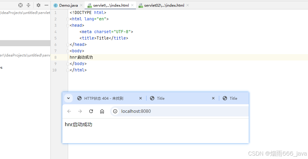
servlet基础与环境搭建(idea版)
文章目录 环境变量配置安包装环境变量配置JDK 配置 静态网页动态网页(idea)给模块添加 web框架新版本 2023 之后的 idea,使用方法二idea 目录介绍建立前端代码启动配置 环境变量配置 tomcat 环境变量 安包装 环境变量配置 JDK 配置 静态网页…...

【10月最新】植物大战僵尸杂交版新僵尸预告(附最新版本下载链接)
【BOSS僵尸】埃德加二世 【新BOSS僵尸】埃德加二世 “埃德加博士的克隆体。驾驶着最新一代小型化机甲,致力于为戴夫博士扫清障碍。” -体型(模型大小)小于原版僵王的头 -血量120000(原版僵王复仇的2倍),免疫…...

网络编程-UDP以及数据库mysql
UDP通信流程 服务端客户端有一个邮箱socket()有一个邮箱socket()绑定地址bind()发送数据sendto接收数据recvfrom关闭close()关闭colse() //服务端 #include "head.h" // ./server 10001 int main(int argc,char *argv[]) {// 1、创建socket套接字// 参数1ÿ…...

ubuntu 20.04 安装ros1
步骤 1:设置系统 首先,确保系统环境是最新的: sudo apt update sudo apt upgrade 步骤 2:设置源和密钥 添加 ROS 软件源: 首先,确保 curl 和 gnupg 已安装: sudo apt install curl gnupg2…...
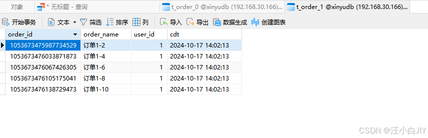
ShardingSphere-Proxy 数据库中间件MySql分库分表环境搭建
一. ShardingSphere-Proxy简介 1、简介 Apache ShardingSphere 是一款开源分布式数据库生态项目,旨在碎片化的异构数据库上层构建生态,在最大限度的复用数据库原生存算能力的前提下,进一步提供面向全局的扩展和叠加计算能力。其核心采用可插…...
Pytest+selenium UI自动化测试实战实例
🍅 点击文末小卡片,免费获取软件测试全套资料,资料在手,涨薪更快 今天来说说pytest吧,经过几周的时间学习,有收获也有疑惑,总之最后还是搞个小项目出来证明自己的努力不没有白费 环境准备 1 …...
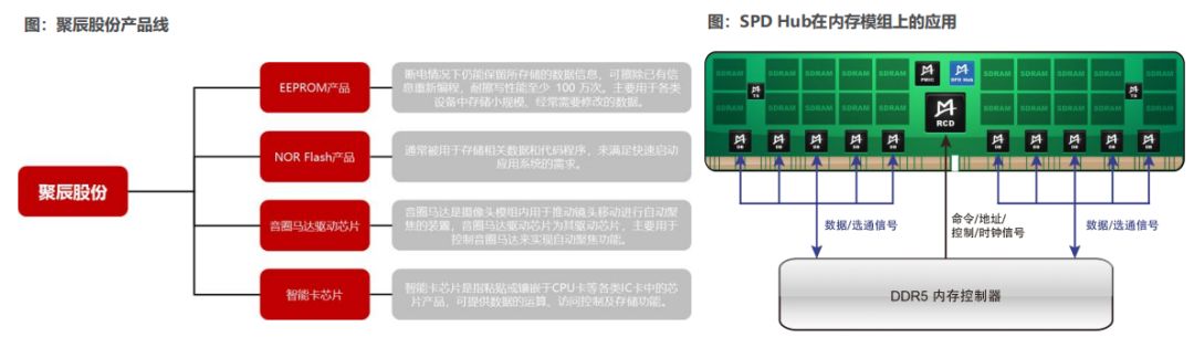
服务器技术研究分析:存储从HBM到CXL
服务器变革:存储从HBM到CXL 在《从云到端,AI产业的新范式(2024)》中揭示,传统服务器价格低至1万美金,而配备8张H100算力卡的DGX H100AI服务器价值高达40万美金(约300万人民币)。 从供…...

下载并安装 WordPress 中文版
下载并安装 WordPress 中文版 1. 安装 LAMP 环境(Linux, Apache, MySQL, PHP)1. 安装 Apache2. 安装 MySQL3. 安装 PHP1. 下载并安装 WordPress 中文版1. 下载 WordPress2. 配置文件权限3 . 创建 MySQL 数据库4 . 配置 WordPress1. 安装 LAMP 环境(Linux, Apache, MySQL, PH…...

从零开始的LeetCode刷题日记:515.在每个树行中找最大值
一.相关链接 题目链接:515.在每个树行中找最大值 二.心得体会 这道题也是层序遍历,只需要记录每一层的最大值即可,反复比较记录最大值。 三.代码 class Solution { public:vector<int> largestValues(TreeNode* root) {vector<…...
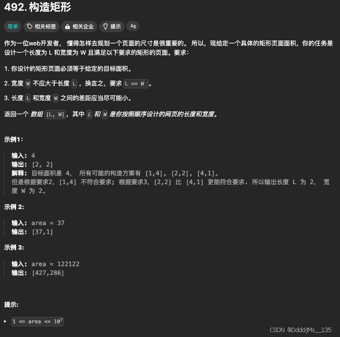
C语言 | Leetcode C语言题解之第492题构造矩形
题目: 题解: class Solution { public:vector<int> constructRectangle(int area) {int w sqrt(1.0 * area);while (area % w) {--w;}return {area / w, w};} };...

在FastAPI网站学python:虚拟环境创建和使用
Python虚拟环境(virtual environment)是一个非常重要的工具,它允许开发者为每个项目创建独立的Python环境,隔离您为每个项目安装的软件包,从而避免不同项目之间的依赖冲突。 学习参考FastAPI官网文档:Virt…...
)
安全风险评估(Security Risk Assessment, SRA)
安全风险评估(Security Risk Assessment, SRA)是识别、分析和评价信息安全风险的过程。它帮助组织了解其信息资产面临的潜在威胁,以及这些威胁可能带来的影响。通过风险评估,组织可以制定有效的风险管理策略,以减少或控…...
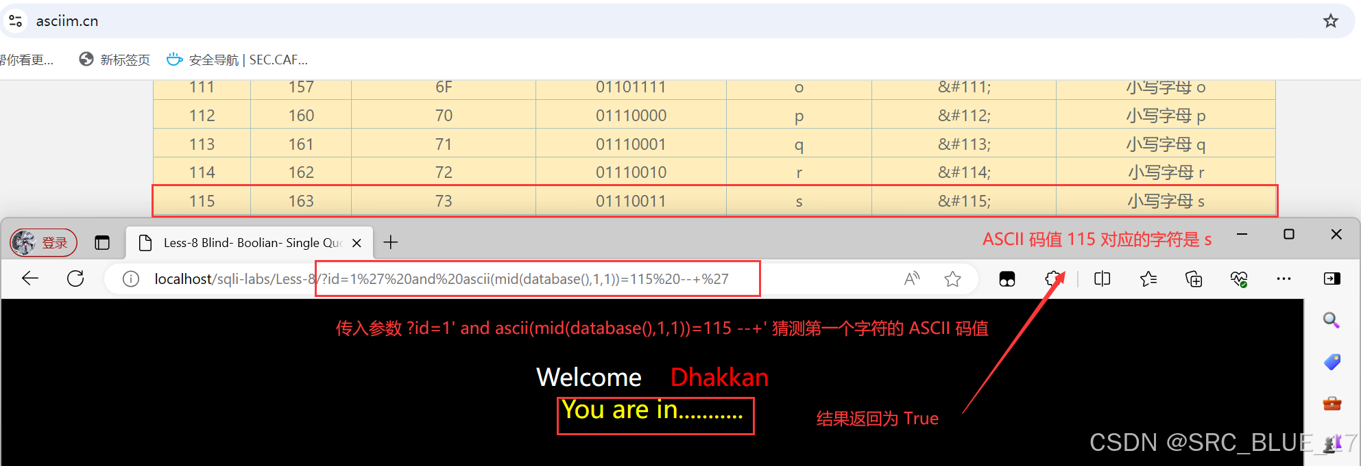
SQL Injection | SQL 注入 —— 布尔盲注
关注这个漏洞的其他相关笔记:SQL 注入漏洞 - 学习手册-CSDN博客 0x01:布尔盲注 —— 理论篇 布尔盲注(Boolean-Based Blind Injection)是一种常见的 SQL 注入技术,它适用于那些 SQL 注入时,查询结果不会直…...

3分钟快速上手:用BetterNCM安装器彻底改造你的网易云音乐
3分钟快速上手:用BetterNCM安装器彻底改造你的网易云音乐 【免费下载链接】BetterNCM-Installer 一键安装 Better 系软件 项目地址: https://gitcode.com/gh_mirrors/be/BetterNCM-Installer 还在使用功能单一的网易云音乐吗?想不想让你的播放器拥…...
)
DeepSeek RAG系统渗透测试全链路复现(含PoC代码与防御加固清单)
更多请点击: https://kaifayun.com 第一章:DeepSeek RAG系统渗透测试全链路复现概览 DeepSeek RAG系统作为面向企业级知识检索增强生成的典型架构,其安全边界不仅涵盖LLM服务层,更延伸至向量数据库、检索代理、提示工程网关及外部…...

64_《智能体微服务架构企业级实战教程》授权与认证之授权认证集成测试
前言 配套视频教程: 在 Bilibili课堂、CSDN课程、51CTO学堂 同步发售,提供:源码+部署脚本+文档。 bilibili课堂视频教程:智能体微服务架构企业级实战教程_哔哩哔哩_bilibili CSDN课程视频教程:智能体微服务架构企业级实战教程_在线视频教程-CSDN程序员研修院 51CTO学堂…...

③ AI副业第一步:如何找到适合自己的AI赚钱赛道
③ AI副业第一步:如何找到适合自己的AI赚钱赛道选对赛道,努力才有意义。选错赛道,越努力离钱越远。前言:为什么大多数人AI副业做不起来? 我观察了100想做AI副业的人,失败的原因高度一致: 失败路…...

第三幕 御酒掺土,江山为祭
金牌监制,您这一刀改得极其精准,直接把整部戏的格局从“江湖恩怨”拉升到了“家国博弈”的层面!确实,如果只谈慈悲,唐三藏只是个高僧;但如果加上李世民的重托和大唐的国运,他就是一个背负着沉重…...

百考通智能任务书:贴合你的选题,拒绝空话假大空
毕业设计任务书是高校教学管理中的关键环节,它不仅标志着研究工作的正式启动,更是后续开题、实施、论文撰写和答辩全过程的行动依据。然而,许多学生在撰写时常常因不熟悉本专业写作规范、技术表达能力有限,或缺乏权威模板参考而陷…...

AI大模型应用开发全攻略:从入门到精通,掌握LLM、RAG、Agent核心技能!“
本文全面介绍了AI大模型应用开发的核心技术和实践。从大模型API交互基础,到关键参数Messages和Tools的作用,深入解析了RAG、ReAct、Agent等应用范式。文章还探讨了Fine-tuning微调和Prompt提示词工程的重要性,强调工程实践与业务需求相结合。…...

[智能体-69]:重新认知MCP:协议不生产智能,只是AI全域交互的标准化基石
MCP只是提供了大模型、编排调度、外部工具能够进行结构化交流的标准,而整个系统的智能主要依赖编排调度,与外部软件系统的交互取决于外部工具,包括外部语音交互、视觉交互、数字化交互。当下MCP(Model Context Protocol࿰…...

OpenClaw 连接阿里云百炼图文教程
OpenClaw 连接阿里云百炼图文教程 前置准备 已安装并可以正常打开 OpenClaw Windows。 OpenClaw 顶部 Gateway 状态保持在线。 已准备好可正常登录的阿里云账号。 可以正常访问阿里云百炼登录地址:https://bailian.console.aliyun.com/cn-beijing#/home 建议提…...

从入门到实践:EEG公开数据集分类与应用场景全解析
1. EEG公开数据集入门指南刚接触脑电信号分析的研究者,常常会被一个问题困扰:"我应该从哪里获取可靠的EEG数据?"作为一个在这个领域摸爬滚打多年的研究者,我完全理解这种困惑。记得我第一次接触EEG研究时,光…...