用 Python 从零开始创建神经网络（十七）：回归（Regression）

引言

到目前为止，我们一直在处理分类模型，目标是确定某个事物是什么。现在我们感兴趣的是基于输入来确定一个具体的数值。例如，你可能希望使用神经网络来预测明天的温度或一辆车的价格。对于这样的任务，我们需要输出更加精细的结果。这也意味着我们需要一种新的方法来衡量损失，并且需要一个新的输出层激活函数！同时，这也意味着我们所用的数据不同。我们需要包含目标标量数值的训练数据，而不是分类数据。

import matplotlib.pyplot as plt
import nnfs
from nnfs.datasets import sine_datannfs.init()X, y = sine_data()plt.plot(X, y)
plt.show()

上面的数据将生成类似的图表：

1. 线性激活（Linear Activation）

由于我们不再使用分类标签，而是要预测一个标量数值，因此我们将对输出层使用线性激活函数。该线性函数不会修改输入，而是将其直接传递到输出：$y=x$。在反向传播过程中，我们已经知道$f(x)=x$的导数是1；因此，我们新线性激活函数的完整类定义为：

# Linear activation
class Activation_Linear:# Forward passdef forward(self, inputs):# Just remember valuesself.inputs = inputsself.output = inputs# Backward passdef backward(self, dvalues):# derivative is 1, 1 * dvalues = dvalues - the chain ruleself.dinputs = dvalues.copy()

这可能会引发一个问题：为什么我们甚至要编写一些什么都不做的代码？在前向传播中，我们只是将输入传递到输出，在反向传播中同样处理梯度，因为为了应用链式法则，我们将传入的梯度乘以导数，而导数为1。我们这样做只是为了完整性和清晰性，以便在模型定义代码中看到输出层的激活函数。从计算时间的角度来看，这几乎不会增加任何处理时间，至少不会显著影响训练时间。

现在我们只需要解决损失函数的问题！

2. 均方误差损失（Mean Squared Error Loss）

由于我们不再使用分类标签，因此无法计算交叉熵。相反，我们需要一些新的方法。回归任务中计算误差的两种主要方法是均方误差（MSE）和平均绝对误差（MAE）。

对于均方误差，我们将预测值和真实值之间的差异取平方（对于多个回归输出，每个输出都会计算差异），然后对这些平方值求平均。

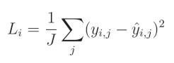
其中，$y$ 表示目标值，$\hat{y}$ 表示预测值，索引 $i$ 表示当前样本，索引 $j$ 表示该样本中的当前输出，$J$ 表示输出的数量。
这里的思想是，偏离目标值越远，惩罚越大。

3. 均方误差损失导数（Mean Squared Error Loss Derivative）

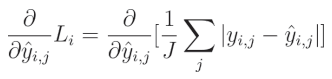
相对于预测值的平方误差偏导数为：

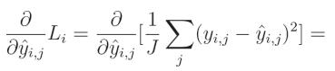
$\frac{1}{J}$（输出数量 $J$ 的倒数）是一个常数，可以移到导数的外部。由于我们是针对给定输出 $j$ 计算导数，因此单个元素的求和结果等于该元素本身。

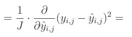
要计算一个表达式的幂的偏导数，我们需要将这个指数与该表达式相乘，然后从指数中减去1，并将其乘以内函数的偏导数：

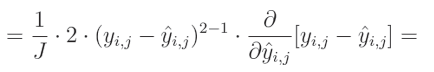
减法的偏导数等于偏导数的减法：

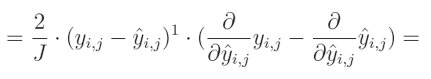
关于真实值对预测值的偏导数等于0，因为我们将其他变量视为常数。而预测值对自身的偏导数等于1，这导致结果为$0-1=-1$。这个结果与方程的其余部分相乘，形成最终解：

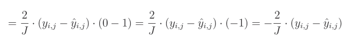
全面解决方案：

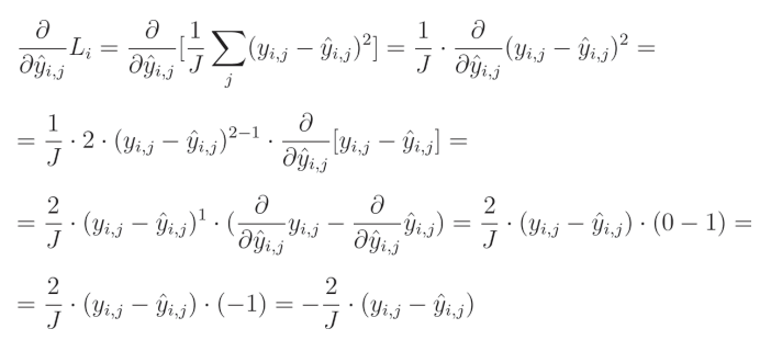
偏导数等于$-2$，再乘以真实值与预测值的差，然后除以输出的数量以对梯度进行归一化，从而使梯度的大小与输出的数量无关。

4. 平均平方误差 (MSE) 损失代码（Mean Squared Error (MSE) Loss Code）

MSE（均方误差）的代码实现包括了用于计算多个输出的样本损失的方程。axis=-1 与均值计算的含义在前一章节中已有详细解释，简而言之，它告诉NumPy对每个样本单独计算输出间的均值。在反向传播中，我们实现了导数方程，其结果为$-2$乘以真实值与预测值之间的差，并除以输出数量进行归一化。与其他损失函数实现类似，我们还对梯度按样本数量进行归一化，使其与批量大小或样本数量无关。

import numpy as np# Mean Squared Error loss
class Loss_MeanSquaredError(Loss): # L2 loss# Forward passdef forward(self, y_pred, y_true):# Calculate losssample_losses = np.mean((y_true - y_pred)**2, axis=-1)# Return lossesreturn sample_losses# Backward passdef backward(self, dvalues, y_true):# Number of samplessamples = len(dvalues)# Number of outputs in every sample# We'll use the first sample to count themoutputs = len(dvalues[0])# Gradient on valuesself.dinputs = -2 * (y_true - dvalues) / outputs# Normalize gradientself.dinputs = self.dinputs / samples

5. 平均绝对误差损失（Mean Absolute Error Loss）

对于平均绝对误差（Mean Absolute Error, MAE），你需要计算单个输出中预测值与真实值之间的绝对差值，然后对这些绝对值求平均：

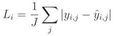
其中，$y$ 表示目标值，$\hat{y}$ 表示预测值，索引 $i$ 表示当前样本，索引 $j$ 表示当前样本中的输出，$J$ 表示输出的数量。

该函数作为损失函数时，对误差进行线性惩罚。它会产生更加稀疏的结果，并对异常值具有较强的鲁棒性，这既可能是优点，也可能是缺点。实际上，L1（MAE）损失的使用频率低于L2（MSE）损失。

6. 平均绝对误差损失导数（Mean Absolute Error Loss Derivative）

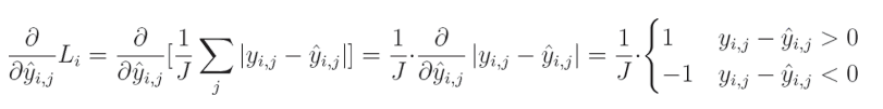
绝对误差相对于预测值的偏导数为：

$1$ 除以 $J$（输出数量）是一个常数，可以移到导数之外。由于我们是对给定输出 $j$ 求导，所以一个元素的和等于该元素本身：

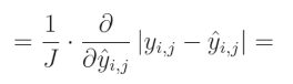
我们之前已经为L1正则化计算了绝对值的偏导数，这与L1损失类似。绝对值的导数在该值大于$0$时等于$1$，在该值小于$0$时等于$-1$。当该值为$0$时，导数不存在：

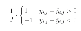
完整解决方案：

7. 平均绝对误差损失代码（Mean Absolute Error Loss Code）

均绝对误差（Mean Absolute Error, MAE）的代码与均方误差（Mean Squared Error, MSE）非常相似。前向传播中使用NumPy的np.abs()函数来计算绝对值，然后再计算均值。反向传播中，我们将使用np.sign()函数，该函数根据输入的符号返回$1$或$-1$，如果参数等于$0$，则返回$0$。接着，我们将梯度根据样本数量进行归一化，使其不受批量大小或样本数量的影响：

import numpy as np# Mean Absolute Error loss
class Loss_MeanAbsoluteError(Loss): # L1 lossdef forward(self, y_pred, y_true):# Calculate losssample_losses = np.mean(np.abs(y_true - y_pred), axis=-1)# Return lossesreturn sample_losses# Backward passdef backward(self, dvalues, y_true):# Number of samplessamples = len(dvalues)# Number of outputs in every sample# We'll use the first sample to count themoutputs = len(dvalues[0])# Calculate gradientself.dinputs = np.sign(y_true - dvalues) / outputs# Normalize gradientself.dinputs = self.dinputs / samples

8. 回归精度（Accuracy in Regression）

既然我们已经有了数据、激活函数和用于回归的损失计算，我们接下来要衡量模型的性能。

在使用交叉熵时，我们可以计算预测与真实目标值相等的情况数，并将其除以样本数量，从而衡量模型的准确率。然而，对于回归模型，我们面临两个问题：

• 第一个问题是，模型中的每个输出神经元（可能有很多）都是单独的输出，这与分类器不同，分类器的所有输出会共同贡献于一个预测结果。
• 第二个问题是，回归模型的预测值是浮点数，我们无法简单地检查输出值是否与真实目标值完全相等，因为它很可能不会相等——即便只有微小的差异，准确率也会被计算为$0$。例如，如果你的模型预测房价，其中某个样本的目标价格是$192,500$，而预测值是$192,495$，那么纯粹的“是否相等”评估会返回False。但考虑到数值的量级，这样的预测在实际中可以被视为“足够接近”或正确。

对于回归任务，没有完美的方法来衡量准确率。但为了直观展示性能，最好还是有一个准确率度量。例如，流行的深度学习框架Keras会同时展示回归模型的准确率和损失，我们也将定义自己的准确率指标。

首先，我们需要一个“限制”值，我们称之为“精度”（precision）。为了计算这个精度，我们将从真实目标值中计算标准差，并将其除以$250$。根据你的目标，这个值可能会有所不同。分母越大，准确率指标就会越“严格”。这里我们选择$250$作为分母。以下是表示这一过程的代码：

accuracy_precision = np.std(y) / 250

然后，我们可以将这个精度值用作回归输出的“容差范围”，在比较目标值和预测值的准确性时起到缓冲作用。我们通过对真实目标值与预测值之间的差异取绝对值来进行比较。接着，我们检查这个差异是否小于我们之前计算得到的精度值：

predictions = activation2.output
accuracy = np.mean(np.absolute(predictions - y) < accuracy_precision)

9. 回归模型训练（Regression Model Training）

有了新的激活函数、损失和计算精度的方法，我们现在就可以创建模型了：

import numpy as np
import nnfs
from nnfs.datasets import spiral_data
from nnfs.datasets import sine_datannfs.init()# Dense layer
class Layer_Dense:# Layer initializationdef __init__(self, n_inputs, n_neurons,weight_regularizer_l1=0, weight_regularizer_l2=0,bias_regularizer_l1=0, bias_regularizer_l2=0):# Initialize weights and biasesself.weights = 0.01 * np.random.randn(n_inputs, n_neurons)self.biases = np.zeros((1, n_neurons))# Set regularization strengthself.weight_regularizer_l1 = weight_regularizer_l1self.weight_regularizer_l2 = weight_regularizer_l2self.bias_regularizer_l1 = bias_regularizer_l1self.bias_regularizer_l2 = bias_regularizer_l2# Forward passdef forward(self, inputs):# Remember input valuesself.inputs = inputs# Calculate output values from inputs, weights and biasesself.output = np.dot(inputs, self.weights) + self.biases# Backward passdef backward(self, dvalues):# Gradients on parametersself.dweights = np.dot(self.inputs.T, dvalues)self.dbiases = np.sum(dvalues, axis=0, keepdims=True)# Gradients on regularization# L1 on weightsif self.weight_regularizer_l1 > 0:dL1 = np.ones_like(self.weights)dL1[self.weights < 0] = -1self.dweights += self.weight_regularizer_l1 * dL1# L2 on weightsif self.weight_regularizer_l2 > 0:self.dweights += 2 * self.weight_regularizer_l2 * self.weights# L1 on biasesif self.bias_regularizer_l1 > 0:dL1 = np.ones_like(self.biases)dL1[self.biases < 0] = -1self.dbiases += self.bias_regularizer_l1 * dL1# L2 on biasesif self.bias_regularizer_l2 > 0:self.dbiases += 2 * self.bias_regularizer_l2 * self.biases# Gradient on valuesself.dinputs = np.dot(dvalues, self.weights.T)# Dropout
class Layer_Dropout:        # Initdef __init__(self, rate):# Store rate, we invert it as for example for dropout# of 0.1 we need success rate of 0.9self.rate = 1 - rate# Forward passdef forward(self, inputs):# Save input valuesself.inputs = inputs# Generate and save scaled maskself.binary_mask = np.random.binomial(1, self.rate, size=inputs.shape) / self.rate# Apply mask to output valuesself.output = inputs * self.binary_mask# Backward passdef backward(self, dvalues):# Gradient on valuesself.dinputs = dvalues * self.binary_mask# ReLU activation
class Activation_ReLU:  # Forward passdef forward(self, inputs):# Remember input valuesself.inputs = inputs# Calculate output values from inputsself.output = np.maximum(0, inputs)# Backward passdef backward(self, dvalues):# Since we need to modify original variable,# let's make a copy of values firstself.dinputs = dvalues.copy()# Zero gradient where input values were negativeself.dinputs[self.inputs <= 0] = 0# Softmax activation
class Activation_Softmax:# Forward passdef forward(self, inputs):# Remember input valuesself.inputs = inputs# Get unnormalized probabilitiesexp_values = np.exp(inputs - np.max(inputs, axis=1, keepdims=True))# Normalize them for each sampleprobabilities = exp_values / np.sum(exp_values, axis=1, keepdims=True)self.output = probabilities# Backward passdef backward(self, dvalues):# Create uninitialized arrayself.dinputs = np.empty_like(dvalues)# Enumerate outputs and gradientsfor index, (single_output, single_dvalues) in enumerate(zip(self.output, dvalues)):# Flatten output arraysingle_output = single_output.reshape(-1, 1)# Calculate Jacobian matrix of the output andjacobian_matrix = np.diagflat(single_output) - np.dot(single_output, single_output.T)# Calculate sample-wise gradient# and add it to the array of sample gradientsself.dinputs[index] = np.dot(jacobian_matrix, single_dvalues)# Sigmoid activation
class Activation_Sigmoid:# Forward passdef forward(self, inputs):# Save input and calculate/save output# of the sigmoid functionself.inputs = inputsself.output = 1 / (1 + np.exp(-inputs))# Backward passdef backward(self, dvalues):# Derivative - calculates from output of the sigmoid functionself.dinputs = dvalues * (1 - self.output) * self.output# Linear activation
class Activation_Linear:# Forward passdef forward(self, inputs):# Just remember valuesself.inputs = inputsself.output = inputs# Backward passdef backward(self, dvalues):# derivative is 1, 1 * dvalues = dvalues - the chain ruleself.dinputs = dvalues.copy()# SGD optimizer
class Optimizer_SGD:# Initialize optimizer - set settings,# learning rate of 1. is default for this optimizerdef __init__(self, learning_rate=1., decay=0., momentum=0.):self.learning_rate = learning_rateself.current_learning_rate = learning_rateself.decay = decayself.iterations = 0self.momentum = momentum# Call once before any parameter updatesdef pre_update_params(self):if self.decay:self.current_learning_rate = self.learning_rate * (1. / (1. + self.decay * self.iterations))# Update parametersdef update_params(self, layer):# If we use momentumif self.momentum:# If layer does not contain momentum arrays, create them# filled with zerosif not hasattr(layer, 'weight_momentums'):layer.weight_momentums = np.zeros_like(layer.weights)# If there is no momentum array for weights# The array doesn't exist for biases yet either.layer.bias_momentums = np.zeros_like(layer.biases)# Build weight updates with momentum - take previous# updates multiplied by retain factor and update with# current gradientsweight_updates = self.momentum * layer.weight_momentums - self.current_learning_rate * layer.dweightslayer.weight_momentums = weight_updates# Build bias updatesbias_updates = self.momentum * layer.bias_momentums - self.current_learning_rate * layer.dbiaseslayer.bias_momentums = bias_updates# Vanilla SGD updates (as before momentum update)else:weight_updates = -self.current_learning_rate * layer.dweightsbias_updates = -self.current_learning_rate * layer.dbiases# Update weights and biases using either# vanilla or momentum updateslayer.weights += weight_updateslayer.biases += bias_updates# Call once after any parameter updatesdef post_update_params(self):self.iterations += 1        # Adagrad optimizer
class Optimizer_Adagrad:# Initialize optimizer - set settingsdef __init__(self, learning_rate=1., decay=0., epsilon=1e-7):self.learning_rate = learning_rateself.current_learning_rate = learning_rateself.decay = decayself.iterations = 0self.epsilon = epsilon# Call once before any parameter updatesdef pre_update_params(self):if self.decay:self.current_learning_rate = self.learning_rate * (1. / (1. + self.decay * self.iterations))# Update parametersdef update_params(self, layer):# If layer does not contain cache arrays,# create them filled with zerosif not hasattr(layer, 'weight_cache'):layer.weight_cache = np.zeros_like(layer.weights)layer.bias_cache = np.zeros_like(layer.biases)# Update cache with squared current gradientslayer.weight_cache += layer.dweights**2layer.bias_cache += layer.dbiases**2# Vanilla SGD parameter update + normalization# with square rooted cachelayer.weights += -self.current_learning_rate * layer.dweights / (np.sqrt(layer.weight_cache) + self.epsilon)layer.biases += -self.current_learning_rate * layer.dbiases / (np.sqrt(layer.bias_cache) + self.epsilon)# Call once after any parameter updatesdef post_update_params(self):self.iterations += 1# RMSprop optimizer
class Optimizer_RMSprop:            # Initialize optimizer - set settingsdef __init__(self, learning_rate=0.001, decay=0., epsilon=1e-7, rho=0.9):self.learning_rate = learning_rateself.current_learning_rate = learning_rateself.decay = decayself.iterations = 0self.epsilon = epsilonself.rho = rho# Call once before any parameter updatesdef pre_update_params(self):if self.decay:self.current_learning_rate = self.learning_rate * (1. / (1. + self.decay * self.iterations))# Update parametersdef update_params(self, layer):# If layer does not contain cache arrays,# create them filled with zerosif not hasattr(layer, 'weight_cache'):layer.weight_cache = np.zeros_like(layer.weights)layer.bias_cache = np.zeros_like(layer.biases)# Update cache with squared current gradientslayer.weight_cache = self.rho * layer.weight_cache + (1 - self.rho) * layer.dweights**2layer.bias_cache = self.rho * layer.bias_cache + (1 - self.rho) * layer.dbiases**2# Vanilla SGD parameter update + normalization# with square rooted cachelayer.weights += -self.current_learning_rate * layer.dweights / (np.sqrt(layer.weight_cache) + self.epsilon)layer.biases += -self.current_learning_rate * layer.dbiases / (np.sqrt(layer.bias_cache) + self.epsilon)# Call once after any parameter updatesdef post_update_params(self):self.iterations += 1# Adam optimizer
class Optimizer_Adam:# Initialize optimizer - set settingsdef __init__(self, learning_rate=0.001, decay=0., epsilon=1e-7, beta_1=0.9, beta_2=0.999):self.learning_rate = learning_rateself.current_learning_rate = learning_rateself.decay = decayself.iterations = 0self.epsilon = epsilonself.beta_1 = beta_1self.beta_2 = beta_2# Call once before any parameter updatesdef pre_update_params(self):if self.decay:self.current_learning_rate = self.learning_rate * (1. / (1. + self.decay * self.iterations))        # Update parametersdef update_params(self, layer):# If layer does not contain cache arrays,# create them filled with zerosif not hasattr(layer, 'weight_cache'):layer.weight_momentums = np.zeros_like(layer.weights)layer.weight_cache = np.zeros_like(layer.weights)layer.bias_momentums = np.zeros_like(layer.biases)layer.bias_cache = np.zeros_like(layer.biases)# Update momentum with current gradientslayer.weight_momentums = self.beta_1 * layer.weight_momentums + (1 - self.beta_1) * layer.dweightslayer.bias_momentums = self.beta_1 * layer.bias_momentums + (1 - self.beta_1) * layer.dbiases# Get corrected momentum# self.iteration is 0 at first pass# and we need to start with 1 hereweight_momentums_corrected = layer.weight_momentums / (1 - self.beta_1 ** (self.iterations + 1))bias_momentums_corrected = layer.bias_momentums / (1 - self.beta_1 ** (self.iterations + 1))# Update cache with squared current gradientslayer.weight_cache = self.beta_2 * layer.weight_cache + (1 - self.beta_2) * layer.dweights**2layer.bias_cache = self.beta_2 * layer.bias_cache + (1 - self.beta_2) * layer.dbiases**2# Get corrected cacheweight_cache_corrected = layer.weight_cache / (1 - self.beta_2 ** (self.iterations + 1))bias_cache_corrected = layer.bias_cache / (1 - self.beta_2 ** (self.iterations + 1))# Vanilla SGD parameter update + normalization# with square rooted cachelayer.weights += -self.current_learning_rate * weight_momentums_corrected / (np.sqrt(weight_cache_corrected) + self.epsilon)layer.biases += -self.current_learning_rate * bias_momentums_corrected / (np.sqrt(bias_cache_corrected) + self.epsilon)# Call once after any parameter updatesdef post_update_params(self):self.iterations += 1# Common loss class
class Loss:# Regularization loss calculationdef regularization_loss(self, layer):        # 0 by defaultregularization_loss = 0# L1 regularization - weights# calculate only when factor greater than 0if layer.weight_regularizer_l1 > 0:regularization_loss += layer.weight_regularizer_l1 * np.sum(np.abs(layer.weights))# L2 regularization - weightsif layer.weight_regularizer_l2 > 0:regularization_loss += layer.weight_regularizer_l2 * np.sum(layer.weights * layer.weights)# L1 regularization - biases# calculate only when factor greater than 0if layer.bias_regularizer_l1 > 0:regularization_loss += layer.bias_regularizer_l1 * np.sum(np.abs(layer.biases))# L2 regularization - biasesif layer.bias_regularizer_l2 > 0:regularization_loss += layer.bias_regularizer_l2 * np.sum(layer.biases * layer.biases)return regularization_loss# Calculates the data and regularization losses# given model output and ground truth valuesdef calculate(self, output, y):# Calculate sample lossessample_losses = self.forward(output, y)# Calculate mean lossdata_loss = np.mean(sample_losses)# Return lossreturn data_loss# Cross-entropy loss
class Loss_CategoricalCrossentropy(Loss):# Forward passdef forward(self, y_pred, y_true):# Number of samples in a batchsamples = len(y_pred)# Clip data to prevent division by 0# Clip both sides to not drag mean towards any valuey_pred_clipped = np.clip(y_pred, 1e-7, 1 - 1e-7)# Probabilities for target values -# only if categorical labelsif len(y_true.shape) == 1:correct_confidences = y_pred_clipped[range(samples),y_true]# Mask values - only for one-hot encoded labelselif len(y_true.shape) == 2:correct_confidences = np.sum(y_pred_clipped * y_true, axis=1)# Lossesnegative_log_likelihoods = -np.log(correct_confidences)return negative_log_likelihoods# Backward passdef backward(self, dvalues, y_true):# Number of samplessamples = len(dvalues)# Number of labels in every sample# We'll use the first sample to count themlabels = len(dvalues[0])# If labels are sparse, turn them into one-hot vectorif len(y_true.shape) == 1:y_true = np.eye(labels)[y_true]# Calculate gradientself.dinputs = -y_true / dvalues# Normalize gradientself.dinputs = self.dinputs / samples# Binary cross-entropy loss
class Loss_BinaryCrossentropy(Loss): # Forward passdef forward(self, y_pred, y_true):# Clip data to prevent division by 0# Clip both sides to not drag mean towards any valuey_pred_clipped = np.clip(y_pred, 1e-7, 1 - 1e-7)# Calculate sample-wise losssample_losses = -(y_true * np.log(y_pred_clipped) + (1 - y_true) * np.log(1 - y_pred_clipped))sample_losses = np.mean(sample_losses, axis=-1)# Return lossesreturn sample_losses       # Backward passdef backward(self, dvalues, y_true):# Number of samplessamples = len(dvalues)# Number of outputs in every sample# We'll use the first sample to count themoutputs = len(dvalues[0])# Clip data to prevent division by 0# Clip both sides to not drag mean towards any valueclipped_dvalues = np.clip(dvalues, 1e-7, 1 - 1e-7)# Calculate gradientself.dinputs = -(y_true / clipped_dvalues - (1 - y_true) / (1 - clipped_dvalues)) / outputs# Normalize gradientself.dinputs = self.dinputs / samples# Mean Squared Error loss
class Loss_MeanSquaredError(Loss): # L2 loss# Forward passdef forward(self, y_pred, y_true):# Calculate losssample_losses = np.mean((y_true - y_pred)**2, axis=-1)# Return lossesreturn sample_losses# Backward passdef backward(self, dvalues, y_true):# Number of samplessamples = len(dvalues)# Number of outputs in every sample# We'll use the first sample to count themoutputs = len(dvalues[0])# Gradient on valuesself.dinputs = -2 * (y_true - dvalues) / outputs# Normalize gradientself.dinputs = self.dinputs / samples# Mean Absolute Error loss
class Loss_MeanAbsoluteError(Loss): # L1 lossdef forward(self, y_pred, y_true):# Calculate losssample_losses = np.mean(np.abs(y_true - y_pred), axis=-1)# Return lossesreturn sample_losses# Backward passdef backward(self, dvalues, y_true):# Number of samplessamples = len(dvalues)# Number of outputs in every sample# We'll use the first sample to count themoutputs = len(dvalues[0])# Calculate gradientself.dinputs = np.sign(y_true - dvalues) / outputs# Normalize gradientself.dinputs = self.dinputs / samples# Softmax classifier - combined Softmax activation
# and cross-entropy loss for faster backward step
class Activation_Softmax_Loss_CategoricalCrossentropy():  # Creates activation and loss function objectsdef __init__(self):self.activation = Activation_Softmax()self.loss = Loss_CategoricalCrossentropy()# Forward passdef forward(self, inputs, y_true):# Output layer's activation functionself.activation.forward(inputs)# Set the outputself.output = self.activation.output# Calculate and return loss valuereturn self.loss.calculate(self.output, y_true)# Backward passdef backward(self, dvalues, y_true):# Number of samplessamples = len(dvalues)     # If labels are one-hot encoded,# turn them into discrete valuesif len(y_true.shape) == 2:y_true = np.argmax(y_true, axis=1)# Copy so we can safely modifyself.dinputs = dvalues.copy()# Calculate gradientself.dinputs[range(samples), y_true] -= 1# Normalize gradientself.dinputs = self.dinputs / samples# Create dataset
X, y = sine_data()# Create Dense layer with 1 input feature and 64 output values
dense1 = Layer_Dense(1, 64)# Create ReLU activation (to be used with Dense layer):
activation1 = Activation_ReLU()# Create second Dense layer with 64 input features (as we take output
# of previous layer here) and 1 output value
dense2 = Layer_Dense(64, 1)
# Create Linear activation:
activation2 = Activation_Linear()# Create loss function
loss_function = Loss_MeanSquaredError()# Create optimizer
optimizer = Optimizer_Adam()# Accuracy precision for accuracy calculation
# There are no really accuracy factor for regression problem,
# but we can simulate/approximate it. We'll calculate it by checking
# how many values have a difference to their ground truth equivalent
# less than given precision
# We'll calculate this precision as a fraction of standard deviation
# of al the ground truth values
accuracy_precision = np.std(y) / 250# Train in loop
for epoch in range(10001):# Perform a forward pass of our training data through this layerdense1.forward(X)# Perform a forward pass through activation function# takes the output of first dense layer hereactivation1.forward(dense1.output)# Perform a forward pass through second Dense layer# takes outputs of activation function# of first layer as inputsdense2.forward(activation1.output)# Perform a forward pass through activation function# takes the output of second dense layer hereactivation2.forward(dense2.output)# Calculate the data lossdata_loss = loss_function.calculate(activation2.output, y)# Calculate regularization penaltyregularization_loss = loss_function.regularization_loss(dense1) + loss_function.regularization_loss(dense2)# Calculate overall lossloss = data_loss + regularization_loss# Calculate accuracy from output of activation2 and targets# To calculate it we're taking absolute difference between# predictions and ground truth values and compare if differences# are lower than given precision valuepredictions = activation2.outputaccuracy = np.mean(np.absolute(predictions - y) < accuracy_precision)if not epoch % 100:print(f'epoch: {epoch}, ' + f'acc: {accuracy:.3f}, ' + f'loss: {loss:.3f} (' + f'data_loss: {data_loss:.3f}, ' + f'reg_loss: {regularization_loss:.3f}), ' + f'lr: {optimizer.current_learning_rate}')# Backward passloss_function.backward(activation2.output, y)activation2.backward(loss_function.dinputs)dense2.backward(activation2.dinputs)activation1.backward(dense2.dinputs)dense1.backward(activation1.dinputs)# Update weights and biasesoptimizer.pre_update_params()optimizer.update_params(dense1)optimizer.update_params(dense2)optimizer.post_update_params()

>>>
epoch: 0, acc: 0.002, loss: 0.500 (data_loss: 0.500, reg_loss: 0.000), lr: 0.001
epoch: 100, acc: 0.003, loss: 0.346 (data_loss: 0.346, reg_loss: 0.000), lr: 0.001
...
epoch: 9900, acc: 0.003, loss: 0.145 (data_loss: 0.145, reg_loss: 0.000), lr: 0.001
epoch: 10000, acc: 0.004, loss: 0.145 (data_loss: 0.145, reg_loss: 0.000), lr: 0.001

这里的训练效果并不理想！让我们添加绘制测试数据的功能，同时对测试数据进行前向传递，在同一张图上绘制输出数据：

import matplotlib.pyplot as pltX_test, y_test = sine_data()dense1.forward(X_test)
activation1.forward(dense1.output)
dense2.forward(activation1.output)
activation2.forward(dense2.output)plt.plot(X_test, y_test)
plt.plot(X_test, activation2.output)
plt.show()

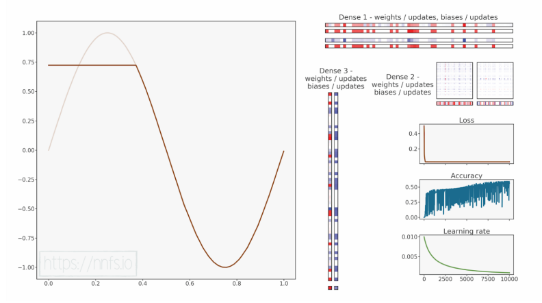
首先，我们导入了matplotlib库，然后创建了一组新的数据。接下来，有4行代码与我们之前代码中前向传播的代码相同。我们可以将其称为预测，或者在我们接下来要讨论的内容中，将其视为验证。我们将在未来的章节中解释验证和预测是什么。目前，理解我们正在做的事情就足够了：我们在与训练模型相同的特征集上进行预测，以查看模型学习到了什么，并返回了什么结果——即输出与训练时的真实目标值有多接近。然后我们绘制训练数据（显然是一个正弦波）和预测数据（我们希望其也形成一个正弦波）。让我们再次运行这段代码，并查看生成的图像：

培训过程动画：

代码可视化：https://nnfs.io/ghi

回顾一下修正线性激活函数（ReLU），它的非线性行为使我们能够映射非线性函数，但我们还需要两个或更多隐藏层。而在这里，我们只有1个隐藏层，后面是输出层。正如我们现在应该知道的那样，这显然是不够的！

如果我们再增加一层：

# Create dataset
X, y = sine_data()# Create Dense layer with 1 input feature and 64 output values
dense1 = Layer_Dense(1, 64)# Create ReLU activation (to be used with Dense layer):
activation1 = Activation_ReLU()# Create second Dense layer with 64 input features (as we take output
# of previous layer here) and 64 output values
dense2 = Layer_Dense(64, 64)# Create ReLU activation (to be used with Dense layer):
activation2 = Activation_ReLU()# Create third Dense layer with 64 input features (as we take output
# of previous layer here) and 1 output value
dense3 = Layer_Dense(64, 1)# Create Linear activation:
activation3 = Activation_Linear()# Create loss function
loss_function = Loss_MeanSquaredError()# Create optimizer
optimizer = Optimizer_Adam()# Accuracy precision for accuracy calculation
# There are no really accuracy factor for regression problem,
# but we can simulate/approximate it. We'll calculate it by checking
# how many values have a difference to their ground truth equivalent
# less than given precision
# We'll calculate this precision as a fraction of standard deviation
# of al the ground truth values
accuracy_precision = np.std(y) / 250# Train in loop
for epoch in range(10001):# Perform a forward pass of our training data through this layerdense1.forward(X)# Perform a forward pass through activation function# takes the output of first dense layer hereactivation1.forward(dense1.output)# Perform a forward pass through second Dense layer# takes outputs of activation function# of first layer as inputsdense2.forward(activation1.output)# Perform a forward pass through activation function# takes the output of second dense layer hereactivation2.forward(dense2.output)# Perform a forward pass through third Dense layer# takes outputs of activation function of second layer as inputsdense3.forward(activation2.output)# Perform a forward pass through activation function# takes the output of third dense layer hereactivation3.forward(dense3.output)# Calculate the data lossdata_loss = loss_function.calculate(activation3.output, y)# Calculate regularization penaltyregularization_loss = loss_function.regularization_loss(dense1) + loss_function.regularization_loss(dense2) + loss_function.regularization_loss(dense3)# Calculate overall lossloss = data_loss + regularization_loss# Calculate accuracy from output of activation2 and targets# To calculate it we're taking absolute difference between# predictions and ground truth values and compare if differences# are lower than given precision valuepredictions = activation3.outputaccuracy = np.mean(np.absolute(predictions - y) < accuracy_precision)if not epoch % 100:print(f'epoch: {epoch}, ' + f'acc: {accuracy:.3f}, ' + f'loss: {loss:.3f} (' + f'data_loss: {data_loss:.3f}, ' + f'reg_loss: {regularization_loss:.3f}), ' + f'lr: {optimizer.current_learning_rate}')# Backward passloss_function.backward(activation3.output, y)activation3.backward(loss_function.dinputs)dense3.backward(activation3.dinputs)activation2.backward(dense3.dinputs)dense2.backward(activation2.dinputs)activation1.backward(dense2.dinputs)dense1.backward(activation1.dinputs)# Update weights and biasesoptimizer.pre_update_params()optimizer.update_params(dense1)optimizer.update_params(dense2)optimizer.update_params(dense3)optimizer.post_update_params()import matplotlib.pyplot as pltX_test, y_test = sine_data()dense1.forward(X_test)
activation1.forward(dense1.output)
dense2.forward(activation1.output)
activation2.forward(dense2.output)
dense3.forward(activation2.output)
activation3.forward(dense3.output)plt.plot(X_test, y_test)
plt.plot(X_test, activation3.output)
plt.show()

>>>
epoch: 0, acc: 0.002, loss: 0.500 (data_loss: 0.500, reg_loss: 0.000), lr: 0.001
epoch: 100, acc: 0.003, loss: 0.187 (data_loss: 0.187, reg_loss: 0.000), lr: 0.001
...
epoch: 9900, acc: 0.617, loss: 0.031 (data_loss: 0.031, reg_loss: 0.000), lr: 0.001
epoch: 10000, acc: 0.620, loss: 0.031 (data_loss: 0.031, reg_loss: 0.000), lr: 0.001

代码可视化：https://nnfs.io/hij

我们的模型准确率并不理想，损失似乎停留在一个较高的水平。从图像中我们可以看到原因，模型在拟合数据时遇到了一些困难，看起来可能卡在了局部最小值。正如我们已经学习过的那样，为了帮助模型跳出局部最小值，我们可以尝试使用更高的学习率并添加学习率衰减。在之前的模型中，我们使用了默认的学习率0.001。现在我们将其设置为0.01，并添加学习率衰减：

optimizer = Optimizer_Adam(learning_rate=0.01, decay=1e-3)

>>>
epoch: 0, acc: 0.002, loss: 0.500 (data_loss: 0.500, reg_loss: 0.000), lr: 0.01
epoch: 100, acc: 0.027, loss: 0.061 (data_loss: 0.061, reg_loss: 0.000), lr: 0.009099181073703368
...
epoch: 9900, acc: 0.565, loss: 0.031 (data_loss: 0.031, reg_loss: 0.000), lr: 0.0009175153683824203
epoch: 10000, acc: 0.564, loss: 0.031 (data_loss: 0.031, reg_loss: 0.000), lr: 0.0009091735612328393

代码可视化：https://nnfs.io/ijk

这次我们的模型似乎仍然停留在更低的准确率上。那就让我们尝试使用更大的学习率吧：

optimizer = Optimizer_Adam(learning_rate=0.05, decay=1e-3)

>>>
epoch: 0, acc: 0.002, loss: 0.500 (data_loss: 0.500, reg_loss: 0.000), lr: 0.05
epoch: 100, acc: 0.087, loss: 0.031 (data_loss: 0.031, reg_loss: 0.000), lr: 0.04549590536851684
...
epoch: 9900, acc: 0.275, loss: 0.031 (data_loss: 0.031, reg_loss: 0.000), lr: 0.004587576841912101
epoch: 10000, acc: 0.229, loss: 0.031 (data_loss: 0.031, reg_loss: 0.000), lr: 0.0045458678061641965

代码可视化：https://nnfs.io/jkl

情况变得更加糟糕了。准确率显著下降，我们可以观察到正弦曲线的下部分形状也变得更差了。似乎我们无法让这个模型学习到数据，但经过多次测试和调整超参数后，我们发现学习率设置为0.005时效果更好：

optimizer = Optimizer_Adam(learning_rate=0.005, decay=1e-3)

>>>
epoch: 0, acc: 0.003, loss: 0.496 (data_loss: 0.496, reg_loss: 0.000), lr: 0.005
epoch: 100, acc: 0.017, loss: 0.048 (data_loss: 0.048, reg_loss: 0.000), lr: 0.004549590536851684
...
epoch: 9900, acc: 0.982, loss: 0.000 (data_loss: 0.000, reg_loss: 0.000), lr: 0.00045875768419121016
epoch: 10000, acc: 0.981, loss: 0.000 (data_loss: 0.000, reg_loss: 0.000), lr: 0.00045458678061641964

代码可视化：https://nnfs.io/klm

这次模型学习得相当不错，但有趣的是，较低或较高的学习率都会导致准确率较低，并且损失值卡在同一位置，而介于它们之间的学习率反而有效。

调试这种问题通常是一项相当困难的任务，且超出了本书的讨论范围。准确率和损失值表明参数的更新幅度不够大，但增加学习率反而使情况变得更糟，我们只能找到这样一个单一的点，让模型能够学习。你可能还记得，在第3章中，我们讨论了参数初始化方法以及为什么要明智地进行初始化。事实证明，在当前情况下，我们可以通过将Dense层中权重初始化的因子从0.01更改为0.1，来帮助模型学习。但你可能会问——既然学习率用于决定应用到参数的梯度幅度，为什么改变这些初始值会有帮助呢？正如你所记得的，反向传播的梯度是使用权重计算的，而学习率不会影响它。这就是为什么使用正确的权重初始化很重要，而到目前为止，我们为每个模型使用的都是相同的值。

例如，如果我们查看Keras（一个神经网络框架）的源代码，我们会发现：

def glorot_uniform(seed=None):"""Glorot uniform initializer, also called Xavier uniform initializer.It draws samples from a uniform distribution within [-limit, limit]where `limit` is `sqrt(6 / (fan_in + fan_out))`where `fan_in` is the number of input units in the weight tensorand `fan_out` is the number of output units in the weight tensor.# Argumentsseed: A Python integer. Used to seed the random generator.# ReturnsAn initializer.# ReferencesGlorot & Bengio, AISTATS 2010http://jmlr.org/proceedings/papers/v9/glorot10a/glorot10a.pdf"""return VarianceScaling(scale=1.,mode='fan_avg',distribution='uniform',seed=seed)

这段代码是Keras 2库的一部分。上述内容中真正重要的是注释部分，它描述了如何初始化权重。我们可以发现有一些重要的信息需要记住——用于乘以均匀分布抽取值的因子取决于输入数量和神经元数量，而不像我们的情况那样是一个常数。这种初始化方法称为Glorot均匀分布（Glorot Uniform）。事实上，我们（本书的作者）在自己的项目中也遇到过非常类似的问题，通过改变权重初始化的方式，使模型从完全无法学习变成能够学习的状态。

对于这个模型的目的，让我们将Dense层中权重初始化的正态分布抽取值的乘数因子改为0.1，并重新运行上述四个尝试，比较结果：

self.weights = 0.1 * np.random.randn(n_inputs, n_neurons)

并重新进行了上述所有测试：

optimizer = Optimizer_Adam()

>>>
epoch: 0, acc: 0.003, loss: 0.496 (data_loss: 0.496, reg_loss: 0.000), lr: 0.001
epoch: 100, acc: 0.005, loss: 0.114 (data_loss: 0.114, reg_loss: 0.000), lr: 0.001
...
epoch: 9900, acc: 0.869, loss: 0.000 (data_loss: 0.000, reg_loss: 0.000), lr: 0.001
epoch: 10000, acc: 0.883, loss: 0.000 (data_loss: 0.000, reg_loss: 0.000), lr: 0.001

代码可视化：https://nnfs.io/lmn

这个模型之前被卡住了，现在已经达到了很高的精度。虽然还有一些明显的瑕疵，比如这个正弦曲线的底边，但整体效果较好。

optimizer = Optimizer_Adam(learning_rate=0.01, decay=1e-3)

>>>
epoch: 0, acc: 0.003, loss: 0.496 (data_loss: 0.496, reg_loss: 0.000), lr: 0.01
epoch: 100, acc: 0.065, loss: 0.011 (data_loss: 0.011, reg_loss: 0.000), lr: 0.009099181073703368
...
epoch: 9900, acc: 0.958, loss: 0.000 (data_loss: 0.000, reg_loss: 0.000), lr: 0.0009175153683824203
epoch: 10000, acc: 0.949, loss: 0.000 (data_loss: 0.000, reg_loss: 0.000), lr: 0.0009091735612328393

代码可视化：https://nnfs.io/mno

另一个以前被卡住的模型这次训练得非常好，达到了非常高的准确率。

optimizer = Optimizer_Adam(learning_rate=0.05, decay=1e-3)

>>>
epoch: 0, acc: 0.003, loss: 0.496 (data_loss: 0.496, reg_loss: 0.000), lr: 0.05
epoch: 100, acc: 0.016, loss: 0.008 (data_loss: 0.008, reg_loss: 0.000), lr: 0.04549590536851684
...
epoch: 9000, acc: 0.802, loss: 0.000 (data_loss: 0.000, reg_loss: 0.000), lr: 0.005000500050005001
epoch: 9100, acc: 0.233, loss: 0.000 (data_loss: 0.000, reg_loss: 0.000), lr: 0.004950985246063967
epoch: 9200, acc: 0.434, loss: 0.000 (data_loss: 0.000, reg_loss: 0.000), lr: 0.004902441415825081
epoch: 9300, acc: 0.838, loss: 0.000 (data_loss: 0.000, reg_loss: 0.000), lr: 0.0048548402757549285
epoch: 9400, acc: 0.309, loss: 0.000 (data_loss: 0.000, reg_loss: 0.000), lr: 0.004808154630252909
epoch: 9500, acc: 0.253, loss: 0.000 (data_loss: 0.000, reg_loss: 0.000), lr: 0.004762358319839985
epoch: 9600, acc: 0.795, loss: 0.000 (data_loss: 0.000, reg_loss: 0.000), lr: 0.004717426172280404
epoch: 9700, acc: 0.802, loss: 0.000 (data_loss: 0.000, reg_loss: 0.000), lr: 0.004673333956444528
epoch: 9800, acc: 0.141, loss: 0.000 (data_loss: 0.000, reg_loss: 0.000), lr: 0.004630058338735069
epoch: 9900, acc: 0.221, loss: 0.000 (data_loss: 0.000, reg_loss: 0.000), lr: 0.004587576841912101
epoch: 10000, acc: 0.631, loss: 0.000 (data_loss: 0.000, reg_loss: 0.000), lr: 0.0045458678061641965

代码可视化：https://nnfs.io/nop

在这种优化器设置下，“跳跃”的准确率表明学习率过大，但即便如此，该模型依然相当不错地学习到了正弦函数的形状。

optimizer = Optimizer_Adam(learning_rate=0.005, decay=1e-3)

>>>
epoch: 0, acc: 0.003, loss: 0.496 (data_loss: 0.496, reg_loss: 0.000), lr: 0.005
epoch: 100, acc: 0.017, loss: 0.048 (data_loss: 0.048, reg_loss: 0.000), lr: 0.004549590536851684
...
epoch: 9900, acc: 0.982, loss: 0.000 (data_loss: 0.000, reg_loss: 0.000), lr: 0.00045875768419121016
epoch: 10000, acc: 0.981, loss: 0.000 (data_loss: 0.000, reg_loss: 0.000), lr: 0.00045458678061641964

代码可视化：https://nnfs.io/opq

这些超参数再次产生了最佳结果，但差距并不大。

正如我们所看到的，这一次我们的模型在所有情况下都学会了，使用不同的学习率时都没有陷入停滞。这说明改变权重初始化对训练过程的影响是多么显著。

到此为止的全部代码：

import numpy as np
import nnfs
from nnfs.datasets import spiral_data
from nnfs.datasets import sine_datannfs.init()# Dense layer
class Layer_Dense:# Layer initializationdef __init__(self, n_inputs, n_neurons,weight_regularizer_l1=0, weight_regularizer_l2=0,bias_regularizer_l1=0, bias_regularizer_l2=0):# Initialize weights and biases# self.weights = 0.01 * np.random.randn(n_inputs, n_neurons)self.weights = 0.1 * np.random.randn(n_inputs, n_neurons)self.biases = np.zeros((1, n_neurons))# Set regularization strengthself.weight_regularizer_l1 = weight_regularizer_l1self.weight_regularizer_l2 = weight_regularizer_l2self.bias_regularizer_l1 = bias_regularizer_l1self.bias_regularizer_l2 = bias_regularizer_l2# Forward passdef forward(self, inputs):# Remember input valuesself.inputs = inputs# Calculate output values from inputs, weights and biasesself.output = np.dot(inputs, self.weights) + self.biases# Backward passdef backward(self, dvalues):# Gradients on parametersself.dweights = np.dot(self.inputs.T, dvalues)self.dbiases = np.sum(dvalues, axis=0, keepdims=True)# Gradients on regularization# L1 on weightsif self.weight_regularizer_l1 > 0:dL1 = np.ones_like(self.weights)dL1[self.weights < 0] = -1self.dweights += self.weight_regularizer_l1 * dL1# L2 on weightsif self.weight_regularizer_l2 > 0:self.dweights += 2 * self.weight_regularizer_l2 * self.weights# L1 on biasesif self.bias_regularizer_l1 > 0:dL1 = np.ones_like(self.biases)dL1[self.biases < 0] = -1self.dbiases += self.bias_regularizer_l1 * dL1# L2 on biasesif self.bias_regularizer_l2 > 0:self.dbiases += 2 * self.bias_regularizer_l2 * self.biases# Gradient on valuesself.dinputs = np.dot(dvalues, self.weights.T)# Dropout
class Layer_Dropout:        # Initdef __init__(self, rate):# Store rate, we invert it as for example for dropout# of 0.1 we need success rate of 0.9self.rate = 1 - rate# Forward passdef forward(self, inputs):# Save input valuesself.inputs = inputs# Generate and save scaled maskself.binary_mask = np.random.binomial(1, self.rate, size=inputs.shape) / self.rate# Apply mask to output valuesself.output = inputs * self.binary_mask# Backward passdef backward(self, dvalues):# Gradient on valuesself.dinputs = dvalues * self.binary_mask# ReLU activation
class Activation_ReLU:  # Forward passdef forward(self, inputs):# Remember input valuesself.inputs = inputs# Calculate output values from inputsself.output = np.maximum(0, inputs)# Backward passdef backward(self, dvalues):# Since we need to modify original variable,# let's make a copy of values firstself.dinputs = dvalues.copy()# Zero gradient where input values were negativeself.dinputs[self.inputs <= 0] = 0# Softmax activation
class Activation_Softmax:# Forward passdef forward(self, inputs):# Remember input valuesself.inputs = inputs# Get unnormalized probabilitiesexp_values = np.exp(inputs - np.max(inputs, axis=1, keepdims=True))# Normalize them for each sampleprobabilities = exp_values / np.sum(exp_values, axis=1, keepdims=True)self.output = probabilities# Backward passdef backward(self, dvalues):# Create uninitialized arrayself.dinputs = np.empty_like(dvalues)# Enumerate outputs and gradientsfor index, (single_output, single_dvalues) in enumerate(zip(self.output, dvalues)):# Flatten output arraysingle_output = single_output.reshape(-1, 1)# Calculate Jacobian matrix of the output andjacobian_matrix = np.diagflat(single_output) - np.dot(single_output, single_output.T)# Calculate sample-wise gradient# and add it to the array of sample gradientsself.dinputs[index] = np.dot(jacobian_matrix, single_dvalues)# Sigmoid activation
class Activation_Sigmoid:# Forward passdef forward(self, inputs):# Save input and calculate/save output# of the sigmoid functionself.inputs = inputsself.output = 1 / (1 + np.exp(-inputs))# Backward passdef backward(self, dvalues):# Derivative - calculates from output of the sigmoid functionself.dinputs = dvalues * (1 - self.output) * self.output# Linear activation
class Activation_Linear:# Forward passdef forward(self, inputs):# Just remember valuesself.inputs = inputsself.output = inputs# Backward passdef backward(self, dvalues):# derivative is 1, 1 * dvalues = dvalues - the chain ruleself.dinputs = dvalues.copy()# SGD optimizer
class Optimizer_SGD:# Initialize optimizer - set settings,# learning rate of 1. is default for this optimizerdef __init__(self, learning_rate=1., decay=0., momentum=0.):self.learning_rate = learning_rateself.current_learning_rate = learning_rateself.decay = decayself.iterations = 0self.momentum = momentum# Call once before any parameter updatesdef pre_update_params(self):if self.decay:self.current_learning_rate = self.learning_rate * (1. / (1. + self.decay * self.iterations))# Update parametersdef update_params(self, layer):# If we use momentumif self.momentum:# If layer does not contain momentum arrays, create them# filled with zerosif not hasattr(layer, 'weight_momentums'):layer.weight_momentums = np.zeros_like(layer.weights)# If there is no momentum array for weights# The array doesn't exist for biases yet either.layer.bias_momentums = np.zeros_like(layer.biases)# Build weight updates with momentum - take previous# updates multiplied by retain factor and update with# current gradientsweight_updates = self.momentum * layer.weight_momentums - self.current_learning_rate * layer.dweightslayer.weight_momentums = weight_updates# Build bias updatesbias_updates = self.momentum * layer.bias_momentums - self.current_learning_rate * layer.dbiaseslayer.bias_momentums = bias_updates# Vanilla SGD updates (as before momentum update)else:weight_updates = -self.current_learning_rate * layer.dweightsbias_updates = -self.current_learning_rate * layer.dbiases# Update weights and biases using either# vanilla or momentum updateslayer.weights += weight_updateslayer.biases += bias_updates# Call once after any parameter updatesdef post_update_params(self):self.iterations += 1        # Adagrad optimizer
class Optimizer_Adagrad:# Initialize optimizer - set settingsdef __init__(self, learning_rate=1., decay=0., epsilon=1e-7):self.learning_rate = learning_rateself.current_learning_rate = learning_rateself.decay = decayself.iterations = 0self.epsilon = epsilon# Call once before any parameter updatesdef pre_update_params(self):if self.decay:self.current_learning_rate = self.learning_rate * (1. / (1. + self.decay * self.iterations))# Update parametersdef update_params(self, layer):# If layer does not contain cache arrays,# create them filled with zerosif not hasattr(layer, 'weight_cache'):layer.weight_cache = np.zeros_like(layer.weights)layer.bias_cache = np.zeros_like(layer.biases)# Update cache with squared current gradientslayer.weight_cache += layer.dweights**2layer.bias_cache += layer.dbiases**2# Vanilla SGD parameter update + normalization# with square rooted cachelayer.weights += -self.current_learning_rate * layer.dweights / (np.sqrt(layer.weight_cache) + self.epsilon)layer.biases += -self.current_learning_rate * layer.dbiases / (np.sqrt(layer.bias_cache) + self.epsilon)# Call once after any parameter updatesdef post_update_params(self):self.iterations += 1# RMSprop optimizer
class Optimizer_RMSprop:            # Initialize optimizer - set settingsdef __init__(self, learning_rate=0.001, decay=0., epsilon=1e-7, rho=0.9):self.learning_rate = learning_rateself.current_learning_rate = learning_rateself.decay = decayself.iterations = 0self.epsilon = epsilonself.rho = rho# Call once before any parameter updatesdef pre_update_params(self):if self.decay:self.current_learning_rate = self.learning_rate * (1. / (1. + self.decay * self.iterations))# Update parametersdef update_params(self, layer):# If layer does not contain cache arrays,# create them filled with zerosif not hasattr(layer, 'weight_cache'):layer.weight_cache = np.zeros_like(layer.weights)layer.bias_cache = np.zeros_like(layer.biases)# Update cache with squared current gradientslayer.weight_cache = self.rho * layer.weight_cache + (1 - self.rho) * layer.dweights**2layer.bias_cache = self.rho * layer.bias_cache + (1 - self.rho) * layer.dbiases**2# Vanilla SGD parameter update + normalization# with square rooted cachelayer.weights += -self.current_learning_rate * layer.dweights / (np.sqrt(layer.weight_cache) + self.epsilon)layer.biases += -self.current_learning_rate * layer.dbiases / (np.sqrt(layer.bias_cache) + self.epsilon)# Call once after any parameter updatesdef post_update_params(self):self.iterations += 1# Adam optimizer
class Optimizer_Adam:# Initialize optimizer - set settingsdef __init__(self, learning_rate=0.001, decay=0., epsilon=1e-7, beta_1=0.9, beta_2=0.999):self.learning_rate = learning_rateself.current_learning_rate = learning_rateself.decay = decayself.iterations = 0self.epsilon = epsilonself.beta_1 = beta_1self.beta_2 = beta_2# Call once before any parameter updatesdef pre_update_params(self):if self.decay:self.current_learning_rate = self.learning_rate * (1. / (1. + self.decay * self.iterations))        # Update parametersdef update_params(self, layer):# If layer does not contain cache arrays,# create them filled with zerosif not hasattr(layer, 'weight_cache'):layer.weight_momentums = np.zeros_like(layer.weights)layer.weight_cache = np.zeros_like(layer.weights)layer.bias_momentums = np.zeros_like(layer.biases)layer.bias_cache = np.zeros_like(layer.biases)# Update momentum with current gradientslayer.weight_momentums = self.beta_1 * layer.weight_momentums + (1 - self.beta_1) * layer.dweightslayer.bias_momentums = self.beta_1 * layer.bias_momentums + (1 - self.beta_1) * layer.dbiases# Get corrected momentum# self.iteration is 0 at first pass# and we need to start with 1 hereweight_momentums_corrected = layer.weight_momentums / (1 - self.beta_1 ** (self.iterations + 1))bias_momentums_corrected = layer.bias_momentums / (1 - self.beta_1 ** (self.iterations + 1))# Update cache with squared current gradientslayer.weight_cache = self.beta_2 * layer.weight_cache + (1 - self.beta_2) * layer.dweights**2layer.bias_cache = self.beta_2 * layer.bias_cache + (1 - self.beta_2) * layer.dbiases**2# Get corrected cacheweight_cache_corrected = layer.weight_cache / (1 - self.beta_2 ** (self.iterations + 1))bias_cache_corrected = layer.bias_cache / (1 - self.beta_2 ** (self.iterations + 1))# Vanilla SGD parameter update + normalization# with square rooted cachelayer.weights += -self.current_learning_rate * weight_momentums_corrected / (np.sqrt(weight_cache_corrected) + self.epsilon)layer.biases += -self.current_learning_rate * bias_momentums_corrected / (np.sqrt(bias_cache_corrected) + self.epsilon)# Call once after any parameter updatesdef post_update_params(self):self.iterations += 1# Common loss class
class Loss:# Regularization loss calculationdef regularization_loss(self, layer):        # 0 by defaultregularization_loss = 0# L1 regularization - weights# calculate only when factor greater than 0if layer.weight_regularizer_l1 > 0:regularization_loss += layer.weight_regularizer_l1 * np.sum(np.abs(layer.weights))# L2 regularization - weightsif layer.weight_regularizer_l2 > 0:regularization_loss += layer.weight_regularizer_l2 * np.sum(layer.weights * layer.weights)# L1 regularization - biases# calculate only when factor greater than 0if layer.bias_regularizer_l1 > 0:regularization_loss += layer.bias_regularizer_l1 * np.sum(np.abs(layer.biases))# L2 regularization - biasesif layer.bias_regularizer_l2 > 0:regularization_loss += layer.bias_regularizer_l2 * np.sum(layer.biases * layer.biases)return regularization_loss# Calculates the data and regularization losses# given model output and ground truth valuesdef calculate(self, output, y):# Calculate sample lossessample_losses = self.forward(output, y)# Calculate mean lossdata_loss = np.mean(sample_losses)# Return lossreturn data_loss# Cross-entropy loss
class Loss_CategoricalCrossentropy(Loss):# Forward passdef forward(self, y_pred, y_true):# Number of samples in a batchsamples = len(y_pred)# Clip data to prevent division by 0# Clip both sides to not drag mean towards any valuey_pred_clipped = np.clip(y_pred, 1e-7, 1 - 1e-7)# Probabilities for target values -# only if categorical labelsif len(y_true.shape) == 1:correct_confidences = y_pred_clipped[range(samples),y_true]# Mask values - only for one-hot encoded labelselif len(y_true.shape) == 2:correct_confidences = np.sum(y_pred_clipped * y_true, axis=1)# Lossesnegative_log_likelihoods = -np.log(correct_confidences)return negative_log_likelihoods# Backward passdef backward(self, dvalues, y_true):# Number of samplessamples = len(dvalues)# Number of labels in every sample# We'll use the first sample to count themlabels = len(dvalues[0])# If labels are sparse, turn them into one-hot vectorif len(y_true.shape) == 1:y_true = np.eye(labels)[y_true]# Calculate gradientself.dinputs = -y_true / dvalues# Normalize gradientself.dinputs = self.dinputs / samples# Binary cross-entropy loss
class Loss_BinaryCrossentropy(Loss): # Forward passdef forward(self, y_pred, y_true):# Clip data to prevent division by 0# Clip both sides to not drag mean towards any valuey_pred_clipped = np.clip(y_pred, 1e-7, 1 - 1e-7)# Calculate sample-wise losssample_losses = -(y_true * np.log(y_pred_clipped) + (1 - y_true) * np.log(1 - y_pred_clipped))sample_losses = np.mean(sample_losses, axis=-1)# Return lossesreturn sample_losses       # Backward passdef backward(self, dvalues, y_true):# Number of samplessamples = len(dvalues)# Number of outputs in every sample# We'll use the first sample to count themoutputs = len(dvalues[0])# Clip data to prevent division by 0# Clip both sides to not drag mean towards any valueclipped_dvalues = np.clip(dvalues, 1e-7, 1 - 1e-7)# Calculate gradientself.dinputs = -(y_true / clipped_dvalues - (1 - y_true) / (1 - clipped_dvalues)) / outputs# Normalize gradientself.dinputs = self.dinputs / samples# Mean Squared Error loss
class Loss_MeanSquaredError(Loss): # L2 loss# Forward passdef forward(self, y_pred, y_true):# Calculate losssample_losses = np.mean((y_true - y_pred)**2, axis=-1)# Return lossesreturn sample_losses# Backward passdef backward(self, dvalues, y_true):# Number of samplessamples = len(dvalues)# Number of outputs in every sample# We'll use the first sample to count themoutputs = len(dvalues[0])# Gradient on valuesself.dinputs = -2 * (y_true - dvalues) / outputs# Normalize gradientself.dinputs = self.dinputs / samples# Mean Absolute Error loss
class Loss_MeanAbsoluteError(Loss): # L1 lossdef forward(self, y_pred, y_true):# Calculate losssample_losses = np.mean(np.abs(y_true - y_pred), axis=-1)# Return lossesreturn sample_losses# Backward passdef backward(self, dvalues, y_true):# Number of samplessamples = len(dvalues)# Number of outputs in every sample# We'll use the first sample to count themoutputs = len(dvalues[0])# Calculate gradientself.dinputs = np.sign(y_true - dvalues) / outputs# Normalize gradientself.dinputs = self.dinputs / samples# Softmax classifier - combined Softmax activation
# and cross-entropy loss for faster backward step
class Activation_Softmax_Loss_CategoricalCrossentropy():  # Creates activation and loss function objectsdef __init__(self):self.activation = Activation_Softmax()self.loss = Loss_CategoricalCrossentropy()# Forward passdef forward(self, inputs, y_true):# Output layer's activation functionself.activation.forward(inputs)# Set the outputself.output = self.activation.output# Calculate and return loss valuereturn self.loss.calculate(self.output, y_true)# Backward passdef backward(self, dvalues, y_true):# Number of samplessamples = len(dvalues)     # If labels are one-hot encoded,# turn them into discrete valuesif len(y_true.shape) == 2:y_true = np.argmax(y_true, axis=1)# Copy so we can safely modifyself.dinputs = dvalues.copy()# Calculate gradientself.dinputs[range(samples), y_true] -= 1# Normalize gradientself.dinputs = self.dinputs / samples# Create dataset
X, y = sine_data()# Create Dense layer with 1 input feature and 64 output values
dense1 = Layer_Dense(1, 64)# Create ReLU activation (to be used with Dense layer):
activation1 = Activation_ReLU()# Create second Dense layer with 64 input features (as we take output
# of previous layer here) and 64 output values
dense2 = Layer_Dense(64, 64)# Create ReLU activation (to be used with Dense layer):
activation2 = Activation_ReLU()# Create third Dense layer with 64 input features (as we take output
# of previous layer here) and 1 output value
dense3 = Layer_Dense(64, 1)# Create Linear activation:
activation3 = Activation_Linear()# Create loss function
loss_function = Loss_MeanSquaredError()# Create optimizer
# optimizer = Optimizer_Adam()
# optimizer = Optimizer_Adam(learning_rate=0.01, decay=1e-3)
# optimizer = Optimizer_Adam(learning_rate=0.05, decay=1e-3)
optimizer = Optimizer_Adam(learning_rate=0.005, decay=1e-3)# Accuracy precision for accuracy calculation
# There are no really accuracy factor for regression problem,
# but we can simulate/approximate it. We'll calculate it by checking
# how many values have a difference to their ground truth equivalent
# less than given precision
# We'll calculate this precision as a fraction of standard deviation
# of al the ground truth values
accuracy_precision = np.std(y) / 250# Train in loop
for epoch in range(10001):# Perform a forward pass of our training data through this layerdense1.forward(X)# Perform a forward pass through activation function# takes the output of first dense layer hereactivation1.forward(dense1.output)# Perform a forward pass through second Dense layer# takes outputs of activation function# of first layer as inputsdense2.forward(activation1.output)# Perform a forward pass through activation function# takes the output of second dense layer hereactivation2.forward(dense2.output)# Perform a forward pass through third Dense layer# takes outputs of activation function of second layer as inputsdense3.forward(activation2.output)# Perform a forward pass through activation function# takes the output of third dense layer hereactivation3.forward(dense3.output)# Calculate the data lossdata_loss = loss_function.calculate(activation3.output, y)# Calculate regularization penaltyregularization_loss = loss_function.regularization_loss(dense1) + loss_function.regularization_loss(dense2) + loss_function.regularization_loss(dense3)# Calculate overall lossloss = data_loss + regularization_loss# Calculate accuracy from output of activation2 and targets# To calculate it we're taking absolute difference between# predictions and ground truth values and compare if differences# are lower than given precision valuepredictions = activation3.outputaccuracy = np.mean(np.absolute(predictions - y) < accuracy_precision)if not epoch % 100:print(f'epoch: {epoch}, ' + f'acc: {accuracy:.3f}, ' + f'loss: {loss:.3f} (' + f'data_loss: {data_loss:.3f}, ' + f'reg_loss: {regularization_loss:.3f}), ' + f'lr: {optimizer.current_learning_rate}')# Backward passloss_function.backward(activation3.output, y)activation3.backward(loss_function.dinputs)dense3.backward(activation3.dinputs)activation2.backward(dense3.dinputs)dense2.backward(activation2.dinputs)activation1.backward(dense2.dinputs)dense1.backward(activation1.dinputs)# Update weights and biasesoptimizer.pre_update_params()optimizer.update_params(dense1)optimizer.update_params(dense2)optimizer.update_params(dense3)optimizer.post_update_params()import matplotlib.pyplot as pltX_test, y_test = sine_data()dense1.forward(X_test)
activation1.forward(dense1.output)
dense2.forward(activation1.output)
activation2.forward(dense2.output)
dense3.forward(activation2.output)
activation3.forward(dense3.output)plt.plot(X_test, y_test)
plt.plot(X_test, activation3.output)
plt.show()

---

本章的章节代码、更多资源和勘误表：https://nnfs.io/ch17