Factorization Machines(论文笔记)
样例一:
一个简单的例子,train是一个字典,先将train进行“one-hot” coding,然后输入相关特征向量,可以预测相关性。
from pyfm import pylibfm
from sklearn.feature_extraction import DictVectorizer
import numpy as np
train = [{"user": "1", "item": "5", "age": 19},{"user": "2", "item": "43", "age": 33},{"user": "3", "item": "20", "age": 55},{"user": "4", "item": "10", "age": 20},
]
v = DictVectorizer()
X = v.fit_transform(train)
print(X.toarray())
y = np.repeat(1.0,X.shape[0])
#print(X.shape[0])
fm = pylibfm.FM()
fm.fit(X,y)
fm.predict(v.transform({"user": "1", "item": "10", "age": 40}))
输出:
[[19.  0.  0.  0.  1.  1.  0.  0.  0.][33.  0.  0.  1.  0.  0.  1.  0.  0.][55.  0.  1.  0.  0.  0.  0.  1.  0.][20.  1.  0.  0.  0.  0.  0.  0.  1.]]
4
Creating validation dataset of 0.01 of training for adaptive regularization
-- Epoch 1
Training log loss: 0.37518
array([0.9999684])
样例二:
是基于真实的电影评分数据来训练。数据集点击下载即可。
import numpy as np
from sklearn.feature_extraction import DictVectorizer
from pyfm import pylibfm# Read in data
def loadData(filename,path="ml-100k/"):data = []y = []users=set()items=set()with open(path+filename) as f:for line in f:(user,movieid,rating,ts)=line.split('\t')data.append({ "user_id": str(user), "movie_id": str(movieid)})y.append(float(rating))users.add(user)items.add(movieid)return (data, np.array(y), users, items)(train_data, y_train, train_users, train_items) = loadData("ua.base")
(test_data, y_test, test_users, test_items) = loadData("ua.test")
v = DictVectorizer()
X_train = v.fit_transform(train_data)
X_test = v.transform(test_data)# Build and train a Factorization Machine
fm = pylibfm.FM(num_factors=10, num_iter=100, verbose=True, task="regression", initial_learning_rate=0.001, learning_rate_schedule="optimal")fm.fit(X_train,y_train)# Evaluate
preds = fm.predict(X_test)
from sklearn.metrics import mean_squared_error
print("FM MSE: %.4f" % mean_squared_error(y_test,preds))
输出:
Creating validation dataset of 0.01 of training for adaptive regularization
-- Epoch 1
Training MSE: 0.59525
-- Epoch 2
Training MSE: 0.51804
-- Epoch 3
Training MSE: 0.49046
-- Epoch 4
Training MSE: 0.47458
-- Epoch 5
Training MSE: 0.46416
-- Epoch 6
Training MSE: 0.45662
-- Epoch 7
Training MSE: 0.45099
-- Epoch 8
Training MSE: 0.44639
-- Epoch 9
Training MSE: 0.44264
-- Epoch 10
Training MSE: 0.43949
-- Epoch 11
Training MSE: 0.43675
-- Epoch 12
Training MSE: 0.43430
-- Epoch 13
Training MSE: 0.43223
-- Epoch 14
Training MSE: 0.43020
-- Epoch 15
Training MSE: 0.42851
-- Epoch 16
Training MSE: 0.42691
-- Epoch 17
Training MSE: 0.42531
-- Epoch 18
Training MSE: 0.42389
-- Epoch 19
Training MSE: 0.42255
-- Epoch 20
Training MSE: 0.42128
-- Epoch 21
Training MSE: 0.42003
-- Epoch 22
Training MSE: 0.41873
-- Epoch 23
Training MSE: 0.41756
-- Epoch 24
Training MSE: 0.41634
-- Epoch 25
Training MSE: 0.41509
-- Epoch 26
Training MSE: 0.41391
-- Epoch 27
Training MSE: 0.41274
-- Epoch 28
Training MSE: 0.41149
-- Epoch 29
Training MSE: 0.41032
-- Epoch 30
Training MSE: 0.40891
-- Epoch 31
Training MSE: 0.40774
-- Epoch 32
Training MSE: 0.40635
-- Epoch 33
Training MSE: 0.40495
-- Epoch 34
Training MSE: 0.40354
-- Epoch 35
Training MSE: 0.40203
-- Epoch 36
Training MSE: 0.40047
-- Epoch 37
Training MSE: 0.39889
-- Epoch 38
Training MSE: 0.39728
-- Epoch 39
Training MSE: 0.39562
-- Epoch 40
Training MSE: 0.39387
-- Epoch 41
Training MSE: 0.39216
-- Epoch 42
Training MSE: 0.39030
-- Epoch 43
Training MSE: 0.38847
-- Epoch 44
Training MSE: 0.38655
-- Epoch 45
Training MSE: 0.38461
-- Epoch 46
Training MSE: 0.38269
-- Epoch 47
Training MSE: 0.38068
-- Epoch 48
Training MSE: 0.37864
-- Epoch 49
Training MSE: 0.37657
-- Epoch 50
Training MSE: 0.37459
-- Epoch 51
Training MSE: 0.37253
-- Epoch 52
Training MSE: 0.37045
-- Epoch 53
Training MSE: 0.36845
-- Epoch 54
Training MSE: 0.36647
-- Epoch 55
Training MSE: 0.36448
-- Epoch 56
Training MSE: 0.36254
-- Epoch 57
Training MSE: 0.36067
-- Epoch 58
Training MSE: 0.35874
-- Epoch 59
Training MSE: 0.35690
-- Epoch 60
Training MSE: 0.35511
-- Epoch 61
Training MSE: 0.35333
-- Epoch 62
Training MSE: 0.35155
-- Epoch 63
Training MSE: 0.34992
-- Epoch 64
Training MSE: 0.34829
-- Epoch 65
Training MSE: 0.34675
-- Epoch 66
Training MSE: 0.34538
-- Epoch 67
Training MSE: 0.34393
-- Epoch 68
Training MSE: 0.34258
-- Epoch 69
Training MSE: 0.34129
-- Epoch 70
Training MSE: 0.34006
-- Epoch 71
Training MSE: 0.33885
-- Epoch 72
Training MSE: 0.33773
-- Epoch 73
Training MSE: 0.33671
-- Epoch 74
Training MSE: 0.33564
-- Epoch 75
Training MSE: 0.33468
-- Epoch 76
Training MSE: 0.33375
-- Epoch 77
Training MSE: 0.33292
-- Epoch 78
Training MSE: 0.33211
-- Epoch 79
Training MSE: 0.33131
-- Epoch 80
Training MSE: 0.33065
-- Epoch 81
Training MSE: 0.33002
-- Epoch 82
Training MSE: 0.32930
-- Epoch 83
Training MSE: 0.32882
-- Epoch 84
Training MSE: 0.32813
-- Epoch 85
Training MSE: 0.32764
-- Epoch 86
Training MSE: 0.32722
-- Epoch 87
Training MSE: 0.32677
-- Epoch 88
Training MSE: 0.32635
-- Epoch 89
Training MSE: 0.32591
-- Epoch 90
Training MSE: 0.32550
-- Epoch 91
Training MSE: 0.32513
-- Epoch 92
Training MSE: 0.32481
-- Epoch 93
Training MSE: 0.32451
-- Epoch 94
Training MSE: 0.32421
-- Epoch 95
Training MSE: 0.32397
-- Epoch 96
Training MSE: 0.32363
-- Epoch 97
Training MSE: 0.32341
-- Epoch 98
Training MSE: 0.32319
-- Epoch 99
Training MSE: 0.32293
-- Epoch 100
Training MSE: 0.32268
FM MSE: 0.8873
样例三:是一个分类的样例
import numpy as np
from sklearn.feature_extraction import DictVectorizer
from sklearn.model_selection import train_test_split
from pyfm import pylibfmfrom sklearn.datasets import make_classificationX, y = make_classification(n_samples=1000,n_features=100, n_clusters_per_class=1)
data = [ {v: k for k, v in dict(zip(i, range(len(i)))).items()}  for i in X]X_train, X_test, y_train, y_test = train_test_split(data, y, test_size=0.1, random_state=42)v = DictVectorizer()
X_train = v.fit_transform(X_train)
X_test = v.transform(X_test)fm = pylibfm.FM(num_factors=50, num_iter=10, verbose=True, task="classification", initial_learning_rate=0.0001, learning_rate_schedule="optimal")fm.fit(X_train,y_train)from sklearn.metrics import log_loss
print("Validation log loss: %.4f" % log_loss(y_test,fm.predict(X_test)))
输出:
Creating validation dataset of 0.01 of training for adaptive regularization
-- Epoch 1
Training log loss: 2.12467
-- Epoch 2
Training log loss: 1.74185
-- Epoch 3
Training log loss: 1.42232
-- Epoch 4
Training log loss: 1.16085
-- Epoch 5
Training log loss: 0.94964
-- Epoch 6
Training log loss: 0.78052
-- Epoch 7
Training log loss: 0.64547
-- Epoch 8
Training log loss: 0.53758
-- Epoch 9
Training log loss: 0.45132
-- Epoch 10
Training log loss: 0.38187
Validation log loss: 1.3678
代码:pyFM/pyfm/pylibfm.py at master · coreylynch/pyFM (github.com)
相关文章:
)
Factorization Machines(论文笔记)
样例一: 一个简单的例子,train是一个字典,先将train进行“one-hot” coding,然后输入相关特征向量,可以预测相关性。 from pyfm import pylibfm from sklearn.feature_extraction import DictVectorizer import numpy as np tra…...
——使用QTimer定时触发槽函数)
Qt开发(5)——使用QTimer定时触发槽函数
实现效果 软件启动之后,开始计时,到达预定时间后,调用其他类的某个函数。 类的分工 BaseType:软件初始化的调用类 FuncType: 功能函数所在类 具体函数 // FuncType.h class FuncType: public QObject {Q_OBJECT public: publ…...
2023年JAVA最新面试题
2023年JAVA最新面试题 1 JavaWeb基础1.1 HashMap的底层实现原理?1.2 HashMap 和 HashTable的异同?1.5 Collection 和 Collections的区别?1.6 Collection接口的两种区别1.7 ArrayList、LinkedList、Vector者的异同?1.8 String、Str…...
(四)RabbitMQ高级特性(消费端限流、利用限流实现不公平分发、消息存活时间、优先级队列
Lison <dreamlison163.com>, v1.0.0, 2023.06.23 RabbitMQ高级特性(消费端限流、利用限流实现不公平分发、消息存活时间、优先级队列 文章目录 RabbitMQ高级特性(消费端限流、利用限流实现不公平分发、消息存活时间、优先级队列消费端限流利用限流…...
Vue如何配置eslint
eslint官网: eslint.bootcss.com eslicate如何配置 1、选择新的配置: 2、选择三个必选项 3、再选择Css预处理器 4、之后选择处理器 5、选择是提交的时候就进行保存模式 6、放到独立的配置文件上去 7、最后一句是将自己的数据存为预设 8、配合console不要出现的规则…...

Elasticsearch查询文档
GET查询索引单个文档 GET /索引/_doc/ID GET /ffbf/_doc/123返回结果如下,查到了有数据"found" : true表示 {"_index" : "ffbf","_type" : "_doc","_id" : "123","_version" : 2...

面向对象编程:多态性的理论与实践
文章目录 1. 修饰词和访问权限2. 多态的概念3. 多态的使用现象4. 多态的问题与解决5. 多态的意义 在面向对象编程中,多态是一个重要的概念,它允许不同的对象以不同的方式响应相同的消息。本文将深入探讨多态的概念及其应用,以及在Java中如何实…...

linux:filezilla root密码登陆
问题: 如题 参考: 亚马逊服务器FileZilla登录失败解决办法_亚马逊云 ssh链接秘钥认证不了 ubuntu拒绝root用户ssh远程登录解决办法 总结: vi /etc/ssh/sshd_config,修改配置: PermitRootLogin yes PasswordAuthenticat…...
在nginx上部署nuxt项目
先安装Node.js 我安的18.17.0。 安装完成后,可以使用cmd,winr然cmd进入,测试是否安装成功。安装在哪个盘都可以测试。 测试 输入node -v 和 npm -v,(中间有空格)出现下图版本提示就是完成了NodeJS的安装…...
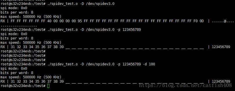
嵌入式linux通用spi驱动之spidev使用总结
Linux内核集成了spidev驱动,提供了SPI设备的用户空间API。支持用于半双工通信的read和write访问接口以及用于全双工通信和I/O配置的ioctl接口。使用时,只需将SPI从设备的compatible属性值添加到spidev区动的spidev dt ids[]数组中,即可将该SP…...

【Nodejs】Puppeteer\爬虫实践
puppeteer 文档:puppeteer.js中文文档|puppeteerjs中文网|puppeteer爬虫教程 Puppeteer本身依赖6.4以上的Node,但是为了异步超级好用的async/await,推荐使用7.6版本以上的Node。另外headless Chrome本身对服务器依赖的库的版本要求比较高,c…...

Windows Active Directory密码同步
大多数 IT 环境中,员工需要记住其默认 Windows Active Directory (AD) 帐户以外的帐户的单独凭据,最重要的是,每个密码还受不同的密码策略和到期日期的约束,为不同的帐户使用单独的密码会增加用户忘记密码和…...
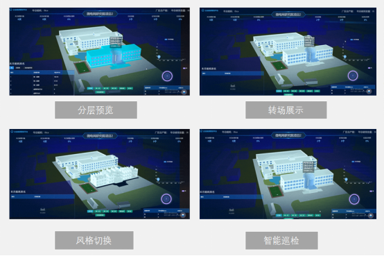
安科瑞能源物联网以能源供应、能源管理、设备管理、能耗分析的能源流向为主线-安科瑞黄安南
摘要:随着科学技术的发展,我国的物联网技术有了很大进展。为了提升电力抄表服务的稳定性,保障电力抄表数据的可靠性,本文提出并实现了基于物联网的智能电力抄表服务平台,结合云计算、大数据等技术,提供电力…...
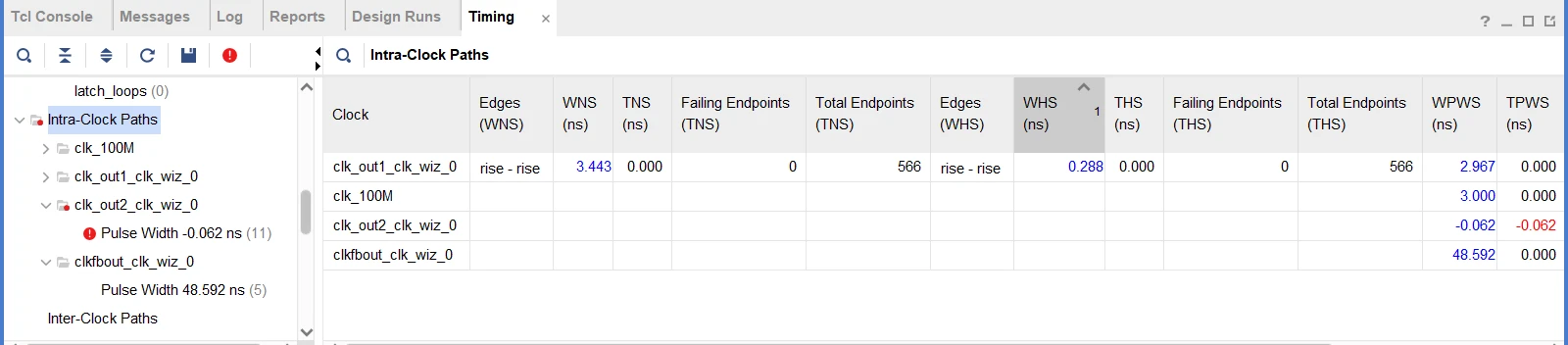
FPGA设计时序分析一、时序路径
目录 一、前言 二、时序路径 2.1 时序路径构成 2.2 时序路径分类 2.3 数据捕获 2.4 Fast corner/Slow corner 2.5 Vivado时序报告 三、参考资料 一、前言 时序路径字面容易简单地理解为时钟路径,事实时钟存在的意义是为了数据的处理、传输,因此严…...
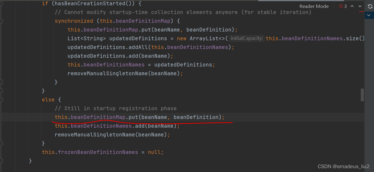
spring复习:(52)注解方式下,ConfigurationClassPostProcessor是怎么被添加到容器的?
进入AnnotationConfigApplicationContext的构造方法: 进入AnnotatedBeanDefinitionReader的构造方法: 进入this(registry, getOrCreateEnvironment(registry));代码如下: 进入AnnotationConfigUtils.registerAnnotationConfigProcessors方…...
全国大学生数据统计与分析竞赛2021年【本科组】-B题:用户消费行为价值分析
目录 摘 要 1 任务背景与重述 1.1 任务背景 1.2 任务重述 2 任务分析 3 数据假设 4 任务求解 4.1 任务一:数据预处理 4.1.1 数据清洗 4.1.2 数据集成 4.1.3 数据变换 4.2 任务二:对用户城市分布情况与分布情况可视化分析 4.2.1 城市分布情况可视化分析 4…...

力扣1667. 修复表中的名字
表: Users ------------------------- | Column Name | Type | ------------------------- | user_id | int | | name | varchar | ------------------------- 在 SQL 中,user_id 是该表的主键。 该表包含用户的 ID 和名字。…...
【设计模式】详解观察者模式
文章目录 1、简介2、观察者模式简单实现抽象主题(Subject)具体主题(ConcreteSubject)抽象观察者(Observer)具体观察者(ConcrereObserver)测试: 观察者设计模式优缺点观察…...

用html+javascript打造公文一键排版系统8:附件及标题排版
最近工作有点忙,所 以没能及时完善公文一键排版系统,现在只好熬夜更新一下。 有时公文有包括附件,招照公文排版规范: 附件应当另面编排,并在版记之前,与公文正文一起装订。“附件”二字及附件顺序号用3号黑…...
微服务体系<1>
我们的微服务架构 我们的微服务架构和单体架构的区别 什么是微服务架构 微服务就是吧我们传统的单体服务分成 订单模块 库存模块 账户模块单体模块 是本地调用 从订单模块 调用到库存模块 再到账户模块 这三个模块都是调用的同一个数据库 这就是我们的单体架构微服务 就是…...

如何高效管理Windows Defender?Defender Control开源工具全解析
如何高效管理Windows Defender?Defender Control开源工具全解析 【免费下载链接】defender-control An open-source windows defender manager. Now you can disable windows defender permanently. 项目地址: https://gitcode.com/gh_mirrors/de/defender-contr…...
真实输出)
SenseVoice-small-ONNX效果展示:情感倾向标注(兴奋/平静/急促)真实输出
SenseVoice-small-ONNX效果展示:情感倾向标注(兴奋/平静/急促)真实输出 1. 核心能力概览 SenseVoice-small-ONNX是一个基于ONNX量化的多语言语音识别模型,它不仅能够准确识别语音内容,还能智能分析说话人的情感倾向。…...

5步构建炉石传说自动化系统:开源工具让日常任务效率提升500%
5步构建炉石传说自动化系统:开源工具让日常任务效率提升500% 【免费下载链接】Hearthstone-Script Hearthstone script(炉石传说脚本) 项目地址: https://gitcode.com/gh_mirrors/he/Hearthstone-Script 炉石传说自动化系统是一款能够…...

OpenClaw+千问3.5-9B低成本方案:自建模型替代OpenAI API
OpenClaw千问3.5-9B低成本方案:自建模型替代OpenAI API 1. 为什么选择自建模型替代OpenAI API 去年冬天的一个深夜,我正在调试一个基于OpenClaw的自动化工作流。当看到账单上OpenAI API调用费用突破四位数时,我意识到必须寻找替代方案。这就…...
。)
Python爬虫入门:10步快速掌握网页数据抓取,【大数据实战】如何从0到1构建用户画像系统(案例+数据仓库+Airflow调度)。
准备工作 安装Python环境,确保版本在3.6以上。推荐使用Anaconda管理Python环境,避免版本冲突。安装必要的库,如requests、BeautifulSoup、lxml等。可以通过pip命令快速安装: pip install requests beautifulsoup4 lxml理解基本概念…...

从Java到Vue的全栈开发之路:一次真实的面试对话
从Java到Vue的全栈开发之路:一次真实的面试对话 在一家互联网大厂的面试中,一位名叫林晨的28岁程序员正接受着技术面试官的提问。他拥有硕士学历,有5年的Java全栈开发经验,曾参与多个大型项目,涉及电商平台、内容社区与…...

24GB显存利用率优化:OpenClaw长任务链对接Qwen3-14B的7个技巧
24GB显存利用率优化:OpenClaw长任务链对接Qwen3-14B的7个技巧 1. 为什么需要关注显存利用率? 上周我尝试用OpenClaw自动化处理一个包含200份PDF文档的信息提取任务时,系统在运行到第37个文件时突然崩溃。查看日志才发现是显存耗尽导致的OOM…...

Django UI扩展全攻略:打造炫酷管理界面,【面试】Kafka / RabbitMQ / ActiveMQ。
Django第三方扩展UI详解:打造现代化管理界面和用户界面 核心UI扩展库介绍 Django-admin-interface 提供高度可定制的管理后台界面,支持主题切换、颜色自定义和模块拖拽布局。无需修改Django原生代码即可实现视觉升级,适合快速构建品牌化管理系…...

学术党福音:OpenClaw+Qwen3-32B自动生成LaTeX论文图表
学术党福音:OpenClawQwen3-32B自动生成LaTeX论文图表 1. 为什么需要自动化论文图表生成 作为长期与LaTeX搏斗的科研狗,我经历过无数次这样的深夜:在Python里调完matplotlib参数,手动导出PNG,再在LaTeX里反复调整\inc…...
)
QT界面设计小技巧:用QListWidget+CheckBox打造可交互列表(避坑指南)
QT界面设计实战:QListWidget与CheckBox的高效交互方案 在桌面应用开发中,列表控件与复选框的组合堪称经典交互模式。这种设计不仅直观地呈现多项选择场景,还能有效提升用户操作效率。作为QT框架中的核心组件,QListWidget与QCheckB…...