Reinforcement Learning with Code 【Chapter 8. Value Funtion Approximation】
Reinforcement Learning with Code
This note records how the author begin to learn RL. Both theoretical understanding and code practice are presented. Many material are referenced such as ZhaoShiyu’s Mathematical Foundation of Reinforcement Learning, .
文章目录
- Reinforcement Learning with Code
- Chapter 8. Value Funtion Approximation
- 8.1 State value: MC/TD learning with function approximation
- 8.2 Action value: Sarsa with funtion approximation
- 8.3 Optimal action value: Q-learning with function approximation
- 8.4 Deep Q-learning (DQN)
- Reference
Chapter 8. Value Funtion Approximation
As so far in this note, state and action values are represented in tabular fashion. There are two problems that first although tabular representation is intuitive, it would encounter some problems when the state action space is large. Second since the value of a state is updated only if it is visited, the values of unvisited states cannot be estimated.
We can sovle the problems using a parameterized function v ^ ( s , w ) \hat{v}(s,w) v^(s,w) to approximate the value funtion, where w ∈ R m w\in\mathbb{R}^m w∈Rm is the parameter vector. On the one hand, we only need to store the parameter w w w instead of all states s s s, which is much smaller. On the other hand, when a state s s s is visited, the parameter w w w is updated so that the values of some other unvisited states can also be estimated.
We usually use neural network to approximate the value function. This problem basically is a regression problem. We can find the optimal parameter w w w by minimize some objective funtions, which we will introduce next.
8.1 State value: MC/TD learning with function approximation
Let v π ( s ) v_\pi(s) vπ(s) and v ^ ( s , w ) \hat{v}(s,w) v^(s,w) be the true value and approximated state value of s ∈ S s\in\mathcal{S} s∈S. The objective funtion considered in value function approximation is usually
J ( w ) = E [ ( v π ( S ) − v ^ ( S , w ) ) 2 ] \textcolor{red}{J(w) = \mathbb{E}\Big[ \big( v_\pi(S)-\hat{v}(S,w) \big)^2 \Big]} J(w)=E[(vπ(S)−v^(S,w))2]
which is also called mean square error in deep learning field. Where S , S ′ S,S^\prime S,S′ denote random variable of state s s s.
Next, we discuss the distribution of random variable S S S. We often use the stationary distribution, which describeds the long-run behavior of a Markov process. Let { d π ( s ) } s ∈ S \textcolor{blue}{\{d_\pi(s)\}_{s\in\mathcal{S}}} {dπ(s)}s∈S donte the stationary distribution of random variable S S S. By definition, d π ( s ) ≥ 0 d_\pi(s)\ge 0 dπ(s)≥0 and ∑ s ∈ S d π ( s ) = 1 \sum_{s\in\mathcal{S}} d_\pi(s)=1 ∑s∈Sdπ(s)=1. Hence, the objective funciton can be rewritten as
J ( w ) = ∑ s ∈ S d π ( s ) [ v π ( s ) − v ^ ( s , w ) ] 2 \textcolor{red}{J(w) = \sum_{s\in\mathcal{S}} d_\pi(s) \Big[v_\pi(s)-\hat{v}(s,w) \Big]^2} J(w)=s∈S∑dπ(s)[vπ(s)−v^(s,w)]2
This objective function is a weighted squared error. How to compute the stationary distribution of random variable S S S? We often use the equation
d π T = d π T P π d_\pi^T = d_\pi^T P_\pi dπT=dπTPπ
As a result, d π d_\pi dπ is the left eigenvector of P π P_\pi Pπ associated with the eigenvalue of 1 1 1. The proof is omitted.
Recall the spirit of gradient descent (GD). We can use it to minimize the objective function as
w k + 1 = w k − α k ∇ w E [ ( v π ( S ) − v ^ ( S , w ) ) 2 ] = w k − α k E [ ∇ w ( v π ( S ) − v ^ ( S , w ) ) 2 ] = w k − 2 α k E [ ( v π ( S ) − v ^ ( S , w ) ) ∇ w ( − v ^ ( S , w ) ) ] = w k + 2 α k E [ v π ( S ) − v ^ ( S , w ) ∇ w v ^ ( S , w ) ] \begin{aligned} w_{k+1} & = w_k - \alpha_k \nabla_w \mathbb{E}\Big[ (v_\pi(S)-\hat{v}(S,w))^2 \Big] \\ & = w_k - \alpha_k \mathbb{E} \Big[ \nabla_w(v_\pi(S)-\hat{v}(S,w))^2 \Big] \\ & = w_k - 2\alpha_k \mathbb{E}\Big[ (v_\pi(S)-\hat{v}(S,w)) \nabla_w(-\hat{v}(S,w)) \Big] \\ & = w_k + 2\alpha_k \mathbb{E} \Big[v_\pi(S)-\hat{v}(S,w) \nabla_w\hat{v}(S,w) \Big] \end{aligned} wk+1=wk−αk∇wE[(vπ(S)−v^(S,w))2]=wk−αkE[∇w(vπ(S)−v^(S,w))2]=wk−2αkE[(vπ(S)−v^(S,w))∇w(−v^(S,w))]=wk+2αkE[vπ(S)−v^(S,w)∇wv^(S,w)]
where without loss of generality the cofficient 2 before α k \alpha_k αk can be dropped. By the spirit of stochastic gradient descent (SGD), we can remove the expectation operation to obtain
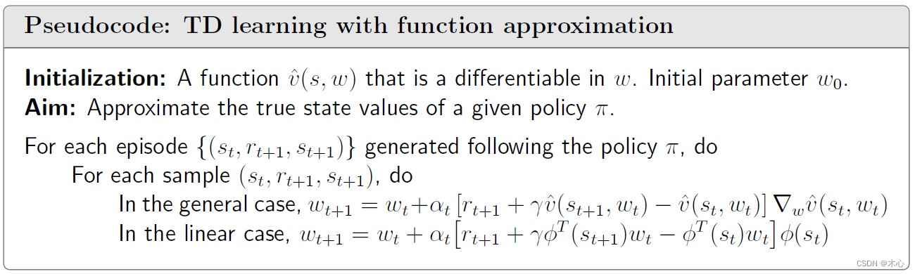
w t + 1 = w t + a t ( v π ( s t ) − v ^ ( s t , w t ) ) ∇ w v ^ ( s t , w t ) w_{t+1} = w_t + a_t (v_\pi(s_t) - \hat{v}(s_t,w_t))\nabla_w \hat{v}(s_t,w_t) wt+1=wt+at(vπ(st)−v^(st,wt))∇wv^(st,wt)
However this equation can’t be implemented. Because it requires the true state value v π v_\pi vπ, which is the unknown to be esitmated. Hence, we can use the idea of Monte Carlo or TD learning to estimate it.
By Monte Carlo learning spirit, we can use the g t g_t gt to denote the discounted return that
g t = r t + 1 + γ r t + 2 + γ 2 r t + 3 + ⋯ g_t = r_{t+1} + \gamma r_{t+2} + \gamma^2 r_{t+3} + \cdots gt=rt+1+γrt+2+γ2rt+3+⋯
Then, g t g_t gt can be used as an approximation of v π ( s ) v_\pi(s) vπ(s). The algorithm becomes
w t + 1 = w t + a t ( g t − v ^ ( s t , w t ) ) ∇ w v ^ ( s t , w t ) w_{t+1} = w_t + a_t (\textcolor{red}{g_t} - \hat{v}(s_t,w_t))\nabla_w \hat{v}(s_t,w_t) wt+1=wt+at(gt−v^(st,wt))∇wv^(st,wt)
By TD learning spirit, we can use the r t + 1 + γ v ^ ( s t + 1 , w t ) r_{t+1}+\gamma \hat{v}(s_{t+1},w_t) rt+1+γv^(st+1,wt) as the approximation of v π ( s ) v_\pi(s) vπ(s). The algorithm becomes
w t + 1 = w t + a t ( r t + 1 + γ v ^ ( s t + 1 , w ) − v ^ ( s t , w t ) ) ∇ w v ^ ( s t , w t ) w_{t+1} = w_t + a_t (\textcolor{red}{r_{t+1}+\gamma \hat{v}(s_{t+1},w)} - \hat{v}(s_t,w_t))\nabla_w \hat{v}(s_t,w_t) wt+1=wt+at(rt+1+γv^(st+1,w)−v^(st,wt))∇wv^(st,wt)
Pesudocode:
8.2 Action value: Sarsa with funtion approximation
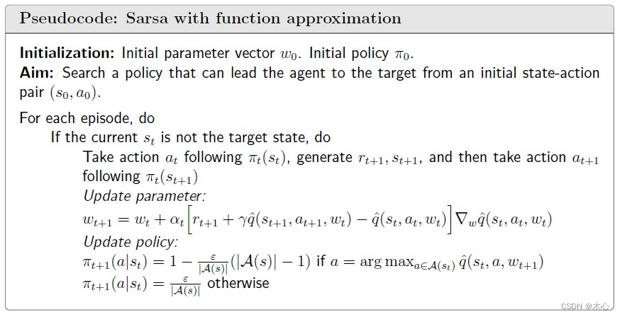
To seach for optimal policies, we need to estimate action values. This section introduces how to estimate action values using Sarsa in the presence of value function approximation.
The action value q π ( s , a ) q_\pi(s,a) qπ(s,a) is described by a function q ^ ( s , a , w ) \hat{q}(s,a,w) q^(s,a,w) parameterized by w w w. The objective funtion considered in action value approximation is usually selected as
J ( w ) = E [ ( q π ( S , A ) − q ^ ( S , A , w ) ) 2 ] \textcolor{red}{J(w) = \mathbb{E}[(q_\pi(S,A) - \hat{q}(S,A,w))^2]} J(w)=E[(qπ(S,A)−q^(S,A,w))2]
Use the stochasitic gradient descent to minimize the objective function
w k + 1 = w k − α k ∇ w E [ ( q π ( S , A ) − q ^ ( S , A , w ) ) 2 ] = w k + 2 a k E [ q π ( S , A ) − q ^ ( S , A , w ) ] ∇ w q ^ ( S , A , w ) = w k + α k ( q π ( s , a ) − q ^ ( s , a , w ) ) ∇ w q ^ ( s , a , w ) \begin{aligned} w_{k+1} & = w_k - \alpha_k \nabla_w \mathbb{E}[(q_\pi(S,A) - \hat{q}(S,A,w))^2] \\ & = w_k + 2a_k \mathbb{E}[q_\pi(S,A) - \hat{q}(S,A,w)]\nabla_w \hat{q}(S,A,w) \\ & = w_k + \alpha_k (q_\pi(s,a) - \hat{q}(s,a,w))\nabla_w\hat{q}(s,a,w) \end{aligned} wk+1=wk−αk∇wE[(qπ(S,A)−q^(S,A,w))2]=wk+2akE[qπ(S,A)−q^(S,A,w)]∇wq^(S,A,w)=wk+αk(qπ(s,a)−q^(s,a,w))∇wq^(s,a,w)
where without loss of generality the cofficient 2 before α k \alpha_k αk can be dropped.
By Sarsa spirit, we use the r + γ q ^ ( s ′ , a ′ , w ) r+\gamma \hat{q}(s^\prime,a^\prime,w) r+γq^(s′,a′,w) to approximate ture action value q π ( s , a ) q_\pi(s,a) qπ(s,a). Hence we have
w k + 1 = w k + α k ( r + γ q ^ ( s ′ , a ′ , w ) − q ^ ( s , a , w ) ) ∇ w q ^ ( s , a , w ) w_{k+1} = w_k + \alpha_k (r+\gamma \hat{q}(s^\prime,a^\prime,w) - \hat{q}(s,a,w))\nabla_w\hat{q}(s,a,w) wk+1=wk+αk(r+γq^(s′,a′,w)−q^(s,a,w))∇wq^(s,a,w)
The sampled data ( s , a , r k , s k ′ , a k ′ ) (s,a,r_k,s^\prime_k,a^\prime_k) (s,a,rk,sk′,ak′) is changed to ( s t , a t , r t + 1 , s t + 1 , a t + 1 ) (s_t,a_t,r_{t+1},s_{t+1},a_{t+1}) (st,at,rt+1,st+1,at+1). Hence
w t + 1 = w t + α t [ r t + 1 + γ q ^ ( s t + 1 , a t + 1 , w t ) − q ^ ( s t , a t , w t ) ] ∇ w q ^ ( s t , a t , w t ) w_{t+1} = w_t + \alpha_t \Big[ \textcolor{red}{r_{t+1}+\gamma \hat{q}(s_{t+1},a_{t+1},w_t)} - \hat{q}(s_t,a_t,w_t) \Big]\nabla_w \hat{q}(s_t,a_t,w_t) wt+1=wt+αt[rt+1+γq^(st+1,at+1,wt)−q^(st,at,wt)]∇wq^(st,at,wt)
Pseudocode:
8.3 Optimal action value: Q-learning with function approximation
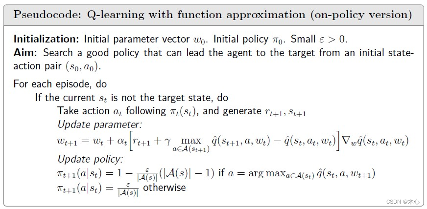
Similar to Sarsa, tabular Q-learning can also be extended to the case of value function approximation.
By the spirit of Q-learning, the update rule is
w t + 1 = w t + α t [ r t + 1 + γ max a ∈ A ( s t + 1 ) q ^ ( s t + 1 , a , w t ) − q ^ ( s t , a t , w t ) ] ∇ w q ^ ( s t , a t , w t ) w_{t+1} = w_t + \alpha_t \Big[ \textcolor{red}{r_{t+1}+\gamma \max_{a\in\mathcal{A}(s_{t+1})} \hat{q}(s_{t+1},a,w_t)} - \hat{q}(s_t,a_t,w_t) \Big]\nabla_w \hat{q}(s_t,a_t,w_t) wt+1=wt+αt[rt+1+γa∈A(st+1)maxq^(st+1,a,wt)−q^(st,at,wt)]∇wq^(st,at,wt)
which is the same as Sarsa expect that q ^ ( s t + 1 , a t + 1 , w t ) \hat{q}(s_{t+1},a_{t+1},w_t) q^(st+1,at+1,wt) is replaced by max a ∈ A ( s t + 1 ) q ^ ( s t + 1 , a , w t ) \max_{a\in\mathcal{A}(s_{t+1})} \hat{q}(s_{t+1},a,w_t) maxa∈A(st+1)q^(st+1,a,wt).
Pseudocode:
8.4 Deep Q-learning (DQN)
We can introduce deep neural networks into Q-learning to obtain deep Q-learning or deep Q-network (DQN).
Mathematically, deep Q-learning aims to minimize the objective funtion
J ( w ) = E [ ( R + γ max a ∈ A ( S ′ ) q ^ ( S ′ , a , w ) − q ^ ( S , A , w ) ) 2 ] \textcolor{red}{J(w) = \mathbb{E} \Big[ \Big( R+\gamma \max_{a\in\mathcal{A}(S^\prime)} \hat{q}(S^\prime, a, w) - \hat{q}(S,A,w) \Big)^2 \Big]} J(w)=E[(R+γa∈A(S′)maxq^(S′,a,w)−q^(S,A,w))2]
where ( S , A , R , S ′ ) (S,A,R,S^\prime) (S,A,R,S′) are random variables representing a state, an action taken at that state, the immediate reward, and the next state. This objective funtion can be viewed as the Bellman opitmality error. That is because
q ( s , a ) = E [ R t + 1 + γ max a ∈ A ( S t + 1 ) q ( S t + 1 , a ) ∣ S t = s , A t = a ] q(s,a) = \mathbb{E} \Big[ R_{t+1} + \gamma \max_{a\in\mathcal{A}(S_{t+1})} q(S_{t+1},a) | S_t = s, A_t= a \Big] q(s,a)=E[Rt+1+γa∈A(St+1)maxq(St+1,a)∣St=s,At=a]
is the Bellman optimality equation in terms of action value.
Then we can use the stochastic gradient to minimize the objective funtion. However, it is noted that the parameter w w w not only apperas in q ^ ( S , A , w ) \hat{q}(S,A,w) q^(S,A,w) but also in y ≜ R + γ max a ∈ A ( S ′ ) q ^ ( S ′ , a , w ) y\triangleq R+\gamma \max_{a\in\mathcal{A}(S^\prime)}\hat{q}(S^\prime,a,w) y≜R+γmaxa∈A(S′)q^(S′,a,w). For the sake of simplicity, we can assume that w w w in y y y is fixed (at least for a while) when we calculate the gradient. To do that, we can introduce two networks. One is a *main networ*k representing q ^ ( s , a , w ) \hat{q}(s,a,w) q^(s,a,w) and the other is a target network q ^ ( s , a , w T ) \hat{q}(s,a,w_T) q^(s,a,wT). The objective function in this case degenerates to
J ( w ) = E [ ( R + γ max a ∈ A ( S ′ ) q ^ ( S ′ , a , w T ) − q ^ ( S , A , w ) ) 2 ] J(w) = \mathbb{E} \Big[ \Big( R+\gamma \max_{a\in\mathcal{A}(S^\prime)} \hat{q}(S^\prime, a, w_T) - \hat{q}(S,A,w) \Big)^2 \Big] J(w)=E[(R+γa∈A(S′)maxq^(S′,a,wT)−q^(S,A,w))2]
where w T w_T wT is the target network parameter and w w w is the main network parameter. When w T w_T wT is fixed, the gradient of J ( w ) J(w) J(w) is
∇ w J = − 2 ∗ E [ ( R + γ max a ∈ A ( S ′ ) q ^ ( S ′ , a , w T ) − q ^ ( S ′ , A , w ) ) ∇ w q ^ ( S , A , w ) ] \nabla_{w}J = -2*\mathbb{E} \Big[ \Big( R + \gamma \max_{a\in\mathcal{A}(S^\prime)} \hat{q}(S^\prime,a,w_T) - \hat{q}(S^\prime,A,w) \Big) \nabla_{w}\hat{q}(S,A,w) \Big] ∇wJ=−2∗E[(R+γa∈A(S′)maxq^(S′,a,wT)−q^(S′,A,w))∇wq^(S,A,w)]
There are two techniques should be noticed.
When the target network is fixed, using stochastic gradient descent (SGD) we can obtain
w t + 1 = w t + α t [ r t + 1 + γ max a ∈ A ( s t + 1 ) q ^ ( s t + 1 , a , w T ) − q ^ ( s t , a t , w ) ] ∇ w q ^ ( s t , a t , w ) \textcolor{red}{w_{t+1} = w_{t} + \alpha_t \Big[ r_{t+1} + \gamma \max_{a\in\mathcal{A}(s_{t+1})} \hat{q}(s_{t+1},a,w_T) - \hat{q}(s_t,a_t,w) \Big] \nabla_w \hat{q}(s_t,a_t,w)} wt+1=wt+αt[rt+1+γa∈A(st+1)maxq^(st+1,a,wT)−q^(st,at,w)]∇wq^(st,at,w)
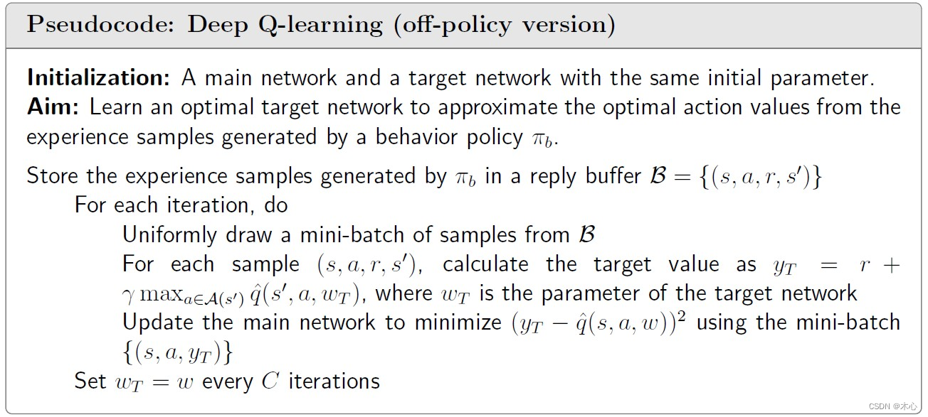
One technique is experience replay. This is, after we have collected some experience samples, we don’t use these samples in the order they were collected. Instead, we store them in a data set, called replay buffer, and draw a batch of samples randomly to train the neureal network. In particular, let ( s , a , r , s ′ ) (s,a,r,s^\prime) (s,a,r,s′) be an experience sample and B ≜ { ( s , a , r , s ′ ) } \mathcal{B}\triangleq \{(s,a,r,s^\prime) \} B≜{(s,a,r,s′)} be the replay buffer. Every time we train the neural network, we can draw a mini-batch of random samples from the reply buffer. The draw of samples, or called experience replay, should follow a uniform distribution.
Another technique is use two networks. A main network parameterized by w w w, and a target network parameterized by w T w_T wT. The two network parameters are set to be the same initially. The target output is y T ≜ r + γ max a ∈ A ( s ′ ) q ^ ( s ′ , a , w T ) y_T \triangleq r + \gamma \max_{a\in\mathcal{A}(s^\prime)}\hat{q}(s^\prime,a,w_T) yT≜r+γmaxa∈A(s′)q^(s′,a,wT). Then, we directly minimize the TD error or called loss function ( y − q ^ ( s , a , w , ) ) 2 (y-\hat{q}(s,a,w,))^2 (y−q^(s,a,w,))2 over the mini-batch { ( s , a , y T ) } \{(s,a,y_T)\} {(s,a,yT)} instead of a single sample to improve efficiency and stability.
The parameter of the main network is updated in every interation. By contrast, the target network is set to be the same as the main network every a certain number of iterations to meet the assumption that w T w_T wT is fixed when calculating the gradient.
Pseudocode:
Reference
赵世钰老师的课程
相关文章:
Reinforcement Learning with Code 【Chapter 8. Value Funtion Approximation】
Reinforcement Learning with Code This note records how the author begin to learn RL. Both theoretical understanding and code practice are presented. Many material are referenced such as ZhaoShiyu’s Mathematical Foundation of Reinforcement Learning, . 文章…...

常用InnoDB参数介绍
常用InnoDB参数介绍 1 状态参数1.1 InnoDB 缓冲池状态监控1.1.1 Innodb_buffer_pool_pages_total1.1.2 Innodb_buffer_pool_pages_data1.1.3 Innodb_buffer_pool_bytes_data1.1.4 Innodb_buffer_pool_pages_dirty1.1.5 Innodb_buffer_pool_bytes_dirty1.1.6 Innodb_buffer_pool…...

云原生网关部署新范式丨 Higress 发布 1.1 版本,支持脱离 K8s 部署
作者:澄潭 版本特性 Higress 1.1.0 版本已经 Release,K8s 环境下可以使用以下命令将 Higress 升级到最新版本: kubectl apply -f https://github.com/alibaba/higress/releases/download/v1.1.0/customresourcedefinitions.gen.yaml helm …...

【通讯录】--C语言
💐 🌸 🌷 🍀 🌹 🌻 🌺 🍁 🍃 🍂 🌿 🍄🍝 🍛 🍤 📃个人主页 :阿然成长日记 …...
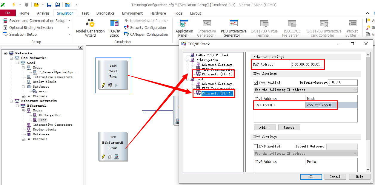
通过两种实现方式理解CANoe TC8 demo是如何判断接收的以太网报文里的字段的
假设有一个测试用例,需求是:编写一个测试用例,发送一条icmpv4 echo request报文给DUT,identifier字段设置为10。判断DUT能够回复icmpv4 echo reply报文,且identifier字段值为10。 实现:在canoe的simulation setup界面插入一个test节点,ip地址为:192.168.0.1,mac地址为…...

Mysql- 存储引擎
目录 1.Mysql体系结构 2.存储引擎简介 3.存储引擎特点 InnoDB MyISAM Memory 4.存储引擎选择 1.Mysql体系结构 MySQL整体的逻辑结构可以分为4层: 连接层:进行相关的连接处理、权限控制、安全处理等操作 服务层:服务层负责与客户层进行…...
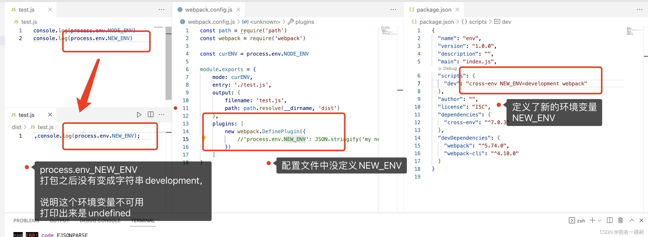
vite / nuxt3 项目使用define配置/自定义,可以使用process.env.xxx获取的环境变量
每日鸡汤:每个你想要学习的瞬间,都是未来的你向自己求救 首先可以看一下我的这篇文章了解一下关于 process.env 的环境变量。 对于vite项目,在我们初始化项目之后,在浏览器中打印 process.env,只有 NODE_ENV这个变量&…...
平台的binutils)
在Linux、Ubuntu中跨平台编译ARM(AARCH64)平台的binutils
Binutils 是GNU(https://www.gnu.org/)提供的一组二进制工具的集合。通常,在已经安装了Linux操作系统的个人电脑上,系统就已经自带了这个工具集。但在进行嵌入式开发的时候,可能会用到支持ARM64平台的Binutils,这时就需要用到交叉编译。 此前,在【1】我们已经介绍过Ubun…...
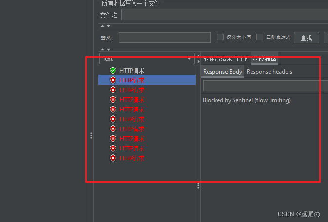
SpringCloudAlibaba微服务实战系列(五)Sentinel1.8.5+Nacos持久化
Sentinel数据持久化 前面介绍Sentinel的流控、熔断降级等功能,同时Sentinel应用也在面临着一个问题:我们在Sentinel后台管理界面中配置了一堆流控、降级规则,但是Sentinel一重启,这些规则全部消失了。那么我们就要考虑Sentinel的持…...

pytest中conftest的用法以及钩子基本使用
一、conftest是什么? conftest是pytest进阶中的高级应用,最近正好用到这一块儿,研究之后,向大家分享该高级应用。 二、使用步骤 1.conftest代码块 以全局性使用driver为主,只启动一次浏览器: pytest.fi…...

数据结构---顺序栈、链栈
特点 typedef struct Stack { int* base; //栈底 int* top;//栈顶 int stacksize //栈的容量; }SqStack; typedef struct StackNode { int data;//数据域 struct StackNode* next; //指针域 }StackNode,*LinkStack; 顺序栈 #define MaxSize 100 typedef struct Stack { int*…...

我的MacBook Pro:维护心得与实用技巧
文章目录 我的MacBook Pro:维护心得与实用技巧工作电脑概况:MacBook Pro 2019款 16 寸日常维护措施个人维护技巧其他建议 我的MacBook Pro:维护心得与实用技巧 无论是学习还是工作,电脑都是IT人必不可少的重要武器。一台好电脑除…...
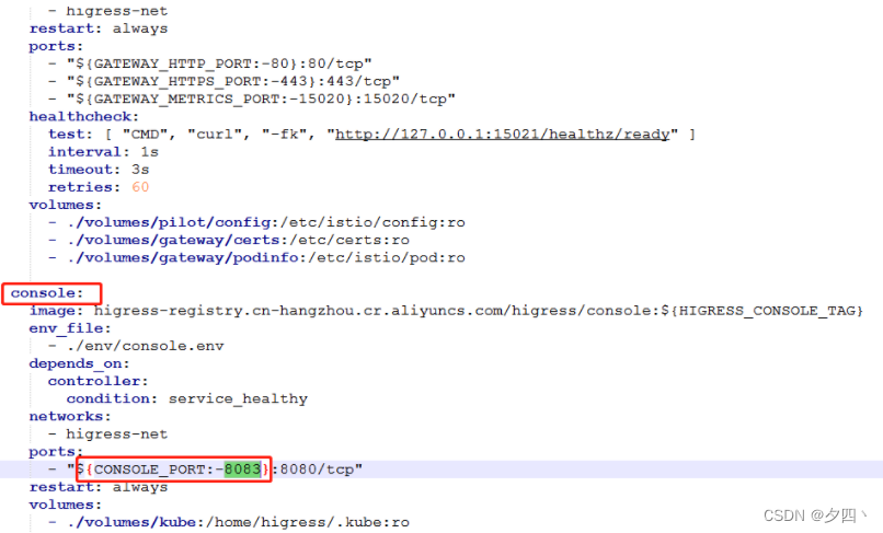
Higress非K8S安装
Higress非K8S安装 文章目录 Higress非K8S安装环境安装安装higress进入到higress 的目录下修改下nacos的地址启动Higress登录higress管理页面 Higress 是基于阿里内部构建的下一代云原生网关,官网介绍:https://higress.io/zh-cn/docs/overview/what-is-hi…...
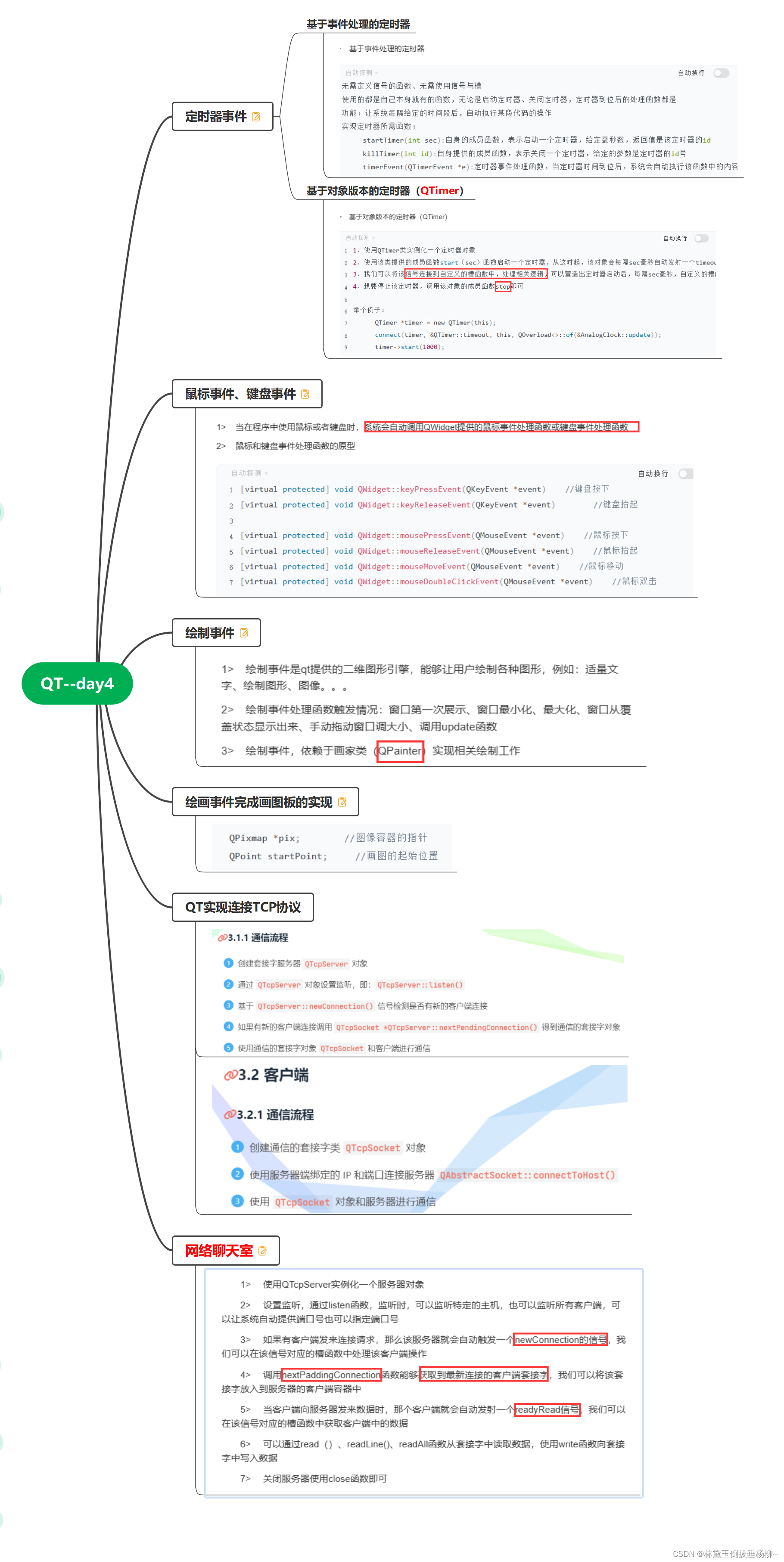
QT--day4(定时器事件、鼠标事件、键盘事件、绘制事件、实现画板、QT实现TCP服务器)
QT实现tcpf服务器代码:(源文件) #include "widget.h" #include "ui_widget.h"Widget::Widget(QWidget *parent): QWidget(parent), ui(new Ui::Widget) {ui->setupUi(this);//给服务器指针实例化空间server new QTc…...

hjm家族信托科技研究报告
目录 绪论 研究背景与意义 一、选题背景 二、选题意义 研究内容与主要研究方法 一、本文内容 二、研究方法 创新与不足 一、创新 二、不足之处 文献综述与理论基础 文献综述 国外研究现状国内研究现状国内外研究综述 理论基础 金融创新理论组合投资理论生命周期理论…...

[SQL挖掘机] - 视图相关操作
创建视图: create view view_name as select column1, column2, ... from table_name where condition;以上语句创建了一个名为view_name的视图,它基于table_name表格,并选择了列column1、column2等作为结果集。可以使用where子句来指定条件。 注意: 视…...
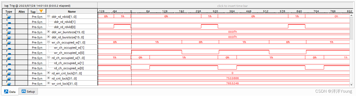
【Quartus FPGA】EMIF DDR3 读写带宽测试
在通信原理中,通信系统的有效性用带宽来衡量,带宽定义为每秒传输的比特数,单位 b/s,或 bps。在 DDR3 接口的产品设计中,DDR3 读/写带宽是设计者必须考虑的指标。本文主要介绍了 Quartus FPGA 平台 EMIF 参数配置&#…...

Flutter:flutter_local_notifications——消息推送的学习
前言 注: 刚开始学习,如果某些案例使用时遇到问题,可以自行百度、查看官方案例、官方github。 简介 Flutter Local Notifications是一个用于在Flutter应用程序中显示本地通知的插件。它提供了一个简单而强大的方法来在设备上发送通知&#…...
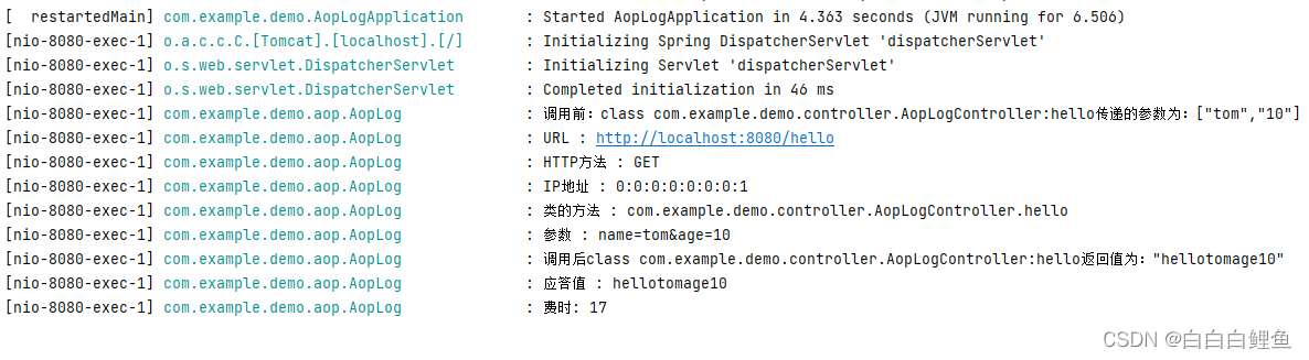
Spring AOP (面向切面编程)原理与代理模式—实例演示
一、AOP介绍和应用场景 Spring 中文文档 (springdoc.cn) Spring | Home 官网 1、AOP介绍(为什么会出现AOP ?) Java是一个面向对象(OOP)的语言,但它有一些弊端。虽然使用OOP可以通过组合或继承的方…...
什么是SCRUM认证体系 ?
Scrum认证是一个针对个人职业发展的认证体系,基础级认证主要面向Scrum的三个角色:Scrum Master、Scrum Product Owner 和 Developers。Scrum认证体系由Scrum官方机构—国际Scrum联盟(ScrumAlliance.org)制定和维护,Scr…...

Realistic Vision V5.1 模型安全与内容过滤部署指南
Realistic Vision V5.1 模型安全与内容过滤部署指南 如果你正在公司里部署AI图像生成服务,最头疼的问题是什么?除了模型效果和生成速度,恐怕就是内容安全了。你肯定不希望员工或者用户用它生成一些不合规的图片,这不仅可能违反公…...

Coze-Loop与Vue3前端性能优化:渲染速度提升方案
Coze-Loop与Vue3前端性能优化:渲染速度提升方案 1. 为什么Vue3项目需要Coze-Loop来诊断性能问题 在实际开发中,很多团队都遇到过这样的困惑:明明代码写得挺规范,但页面滚动卡顿、列表加载缓慢、交互响应迟滞。我们曾接手一个电商…...

MATLAB伪彩色增强实战:从灰度分层到频域处理的完整指南
1. 伪彩色增强技术入门指南 第一次接触伪彩色增强是在研究生课题中,当时需要分析一批医学X光片。盯着那些灰蒙蒙的片子看了三天后,我突然意识到:人眼对色彩差异的敏感度,确实远超对灰度变化的感知。这就是伪彩色技术的核心价值——…...

RVC效果对比实测:原声vs克隆声,你能听出区别吗?
RVC效果对比实测:原声vs克隆声,你能听出区别吗? 1. 引言:AI语音克隆技术的新突破 想象一下,你最喜欢的歌手正在用你的声音唱歌,或者你的播客节目突然有了专业播音员的音色。这不再是科幻场景,…...

新手福音:利用快马一键生成mobaxterm中文界面配置脚本
作为一个经常需要远程连接服务器的用户,MobaXterm一直是我的主力工具之一。但刚开始使用时,全英文的界面确实让我这个新手有点手足无措。最近发现用InsCode(快马)平台可以快速生成配置脚本,简直不要太方便! 为什么需要中文界面 对…...

MiddleBury与SceneFlow数据集相机参数解析与深度图生成实战
1. MiddleBury与SceneFlow数据集简介 MiddleBury和SceneFlow是计算机视觉领域两个非常重要的立体视觉数据集。MiddleBury数据集由Middlebury College发布,包含了大量高质量的立体图像对,这些图像对由两台相机在同一时间、不同位置拍摄,涵盖了…...

VSCode安装与Qwen3开发环境配置一站式解决方案
VSCode安装与Qwen3开发环境配置一站式解决方案 为智能字幕开发量身打造的高效开发环境配置指南 1. 开篇:为什么需要专门的环境配置? 你是不是也遇到过这样的情况:好不容易下载了代码,却发现各种依赖报错,环境配置折腾…...

OpenClaw学习路径:从nanobot镜像入门到开发自定义技能
OpenClaw学习路径:从nanobot镜像入门到开发自定义技能 1. 为什么选择OpenClaw作为自动化助手 第一次听说OpenClaw时,我正在为重复性的文件整理工作头疼。作为一个经常需要处理大量技术文档的开发者,每天要花费数小时在机械的文件分类、重命…...

M2LOrder模型跨操作系统部署:从Windows到Linux的兼容性实战
M2LOrder模型跨操作系统部署:从Windows到Linux的兼容性实战 你是不是也遇到过这种情况?在Windows电脑上跑得好好的一个AI服务,想迁移到Linux服务器上,结果各种报错,环境依赖、路径问题、权限设置……折腾半天也搞不定…...

YOLO X Layout中小企业应用:无需训练,开箱即用的文档结构理解AI工具
YOLO X Layout中小企业应用:无需训练,开箱即用的文档结构理解AI工具 1. 引言:让文档理解变得简单高效 在日常办公中,我们经常需要处理各种文档——扫描的合同、拍摄的表格、电子版报告。传统方式需要人工逐个识别文档中的文字、…...