【机器学习】Feature Engineering and Polynomial Regression
Feature Engineering and Polynomial Regression
- 1. 多项式特征
- 2. 选择特征
- 3. 缩放特征
- 4. 复杂函数
- 附录
首先,导入所需的库:
import numpy as np
import matplotlib.pyplot as plt
from lab_utils_multi import zscore_normalize_features, run_gradient_descent_feng
np.set_printoptions(precision=2)  # reduced display precision on numpy arrays
线性回归模型表示为:
f w , b = w 0 x 0 + w 1 x 1 + . . . + w n − 1 x n − 1 + b (1) f_{\mathbf{w},b} = w_0x_0 + w_1x_1+ ... + w_{n-1}x_{n-1} + b \tag{1} fw,b=w0x0+w1x1+...+wn−1xn−1+b(1)
思考一下,如果特征是非线性的或者是特征的结合,线性模型不能拟合,那该怎么办?
1. 多项式特征
尝试使用目前已知的知识来拟合非线性曲线。我们将从一个简单的二次方程开始: y = 1 + x 2 y = 1+x^2 y=1+x2
# create target data
x = np.arange(0, 20, 1)
y = 1 + x**2
X = x.reshape(-1, 1)model_w,model_b = run_gradient_descent_feng(X,y,iterations=1000, alpha = 1e-2)plt.scatter(x, y, marker='x', c='r', label="Actual Value"); plt.title("no feature engineering")
plt.plot(x,X@model_w + model_b, label="Predicted Value");  plt.xlabel("X"); plt.ylabel("y"); plt.legend(); plt.show()
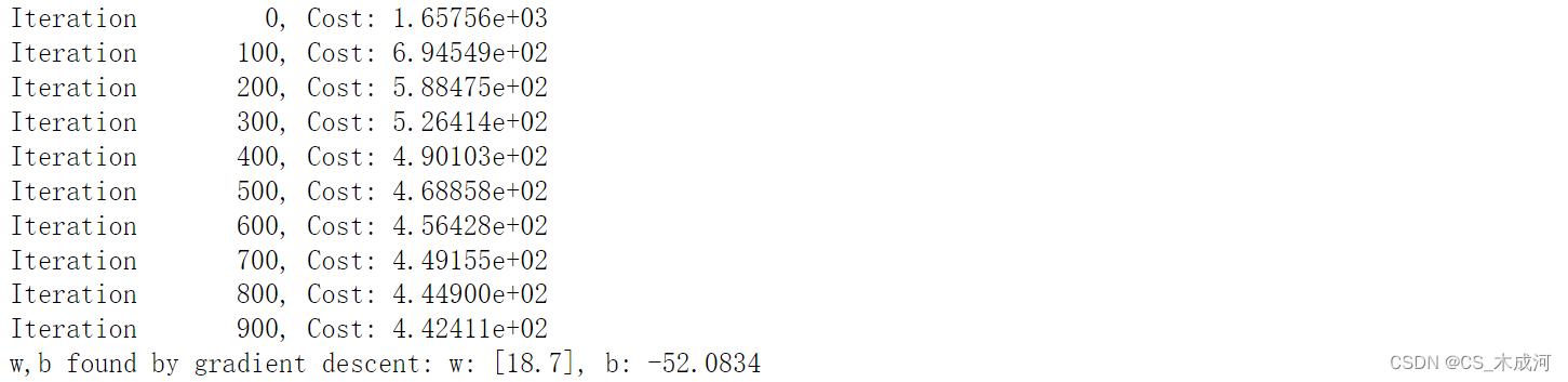
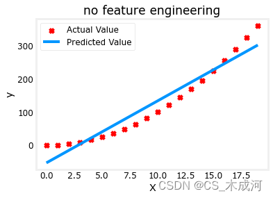
正如所期待的那样,线性方程明显不合适。如果将X 换成 X**2会如何?
# create target data
x = np.arange(0, 20, 1)
y = 1 + x**2# Engineer features
X = x**2      #<-- added engineered feature
X = X.reshape(-1, 1)  #X should be a 2-D Matrix
model_w,model_b = run_gradient_descent_feng(X, y, iterations=10000, alpha = 1e-5)plt.scatter(x, y, marker='x', c='r', label="Actual Value"); plt.title("Added x**2 feature")
plt.plot(x, np.dot(X,model_w) + model_b, label="Predicted Value"); plt.xlabel("x"); plt.ylabel("y"); plt.legend(); plt.show()
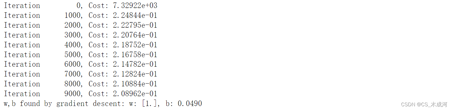
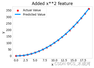
梯度下降将 w , b \mathbf{w},b w,b的初始值修改为 (1.0,0.049) ,即模型方程 y = 1 ∗ x 0 2 + 0.049 y=1*x_0^2+0.049 y=1∗x02+0.049, 这非常接近目标方程 y = 1 ∗ x 0 2 + 1 y=1*x_0^2+1 y=1∗x02+1.
2. 选择特征
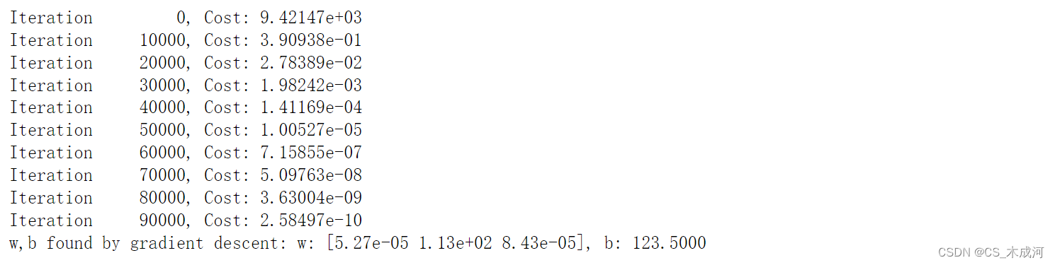
从上面可以知道, x 2 x^2 x2是需要的。接下来我们尝试: y = w 0 x 0 + w 1 x 1 2 + w 2 x 2 3 + b y=w_0x_0 + w_1x_1^2 + w_2x_2^3+b y=w0x0+w1x12+w2x23+b
# create target data
x = np.arange(0, 20, 1)
y = x**2# engineer features .
X = np.c_[x, x**2, x**3]   #<-- added engineered feature
model_w,model_b = run_gradient_descent_feng(X, y, iterations=10000, alpha=1e-7)plt.scatter(x, y, marker='x', c='r', label="Actual Value"); plt.title("x, x**2, x**3 features")
plt.plot(x, X@model_w + model_b, label="Predicted Value"); plt.xlabel("x"); plt.ylabel("y"); plt.legend(); plt.show()
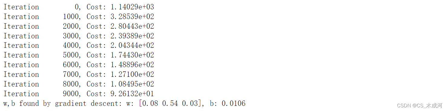
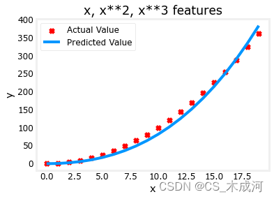
w \mathbf{w} w的值为 [0.08 0.54 0.03] , b 为 0.0106。训练后的模型为:
0.08 x + 0.54 x 2 + 0.03 x 3 + 0.0106 0.08x + 0.54x^2 + 0.03x^3 + 0.0106 0.08x+0.54x2+0.03x3+0.0106
梯度下降通过相对于其他项增加 w 1 w_1 w1项,强调了最适合 x 2 x^2 x2的数据。如果运行很长时间,它将继续减少其他项的影响。梯度下降通过强调其相关参数来为我们选择“正确”的特征。
- 一般来讲,特征被重新缩放,因此它们可以相互比较
- 权重值越小意味着不太重要的特征,在极端情况下,当权重变为零或非常接近零时,相关特征在将模型拟合到数据中是有用的。
- 如上所述,拟合后,与 x 2 x^2 x2功能相关的权重远大于 x x x或 x 3 x^3 x3的权重,因为它在拟合数据时最有用。
多项式特征是根据它们与目标数据的匹配程度来选择的。一旦我们创建了新特征,我们仍然使用线性回归。最好的特征将相对于目标呈线性关系。下面通过一个例子来理解这一点。
# create target data
x = np.arange(0, 20, 1)
y = x**2# engineer features .
X = np.c_[x, x**2, x**3]   #<-- added engineered feature
X_features = ['x','x^2','x^3']
fig,ax=plt.subplots(1, 3, figsize=(12, 3), sharey=True)
for i in range(len(ax)):ax[i].scatter(X[:,i],y)ax[i].set_xlabel(X_features[i])
ax[0].set_ylabel("y")
plt.show()
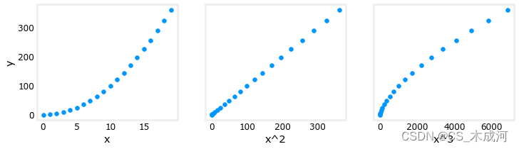
很明显, x 2 x^2 x2特征映射到目标值 y y y是线性的。线性回归可以使用该特征轻松生成模型。
3. 缩放特征
如果数据集具有显着不同尺度的特征,则应该应用特征缩放来加速梯度下降。在上面的例子中,有 x x x, x 2 x^2 x2 和 x 3 x^3 x3,这自然会有非常不同的规模。接下来将 Z-score 归一化应用到示例中。
# create target data
x = np.arange(0,20,1)
X = np.c_[x, x**2, x**3]
print(f"Peak to Peak range by column in Raw        X:{np.ptp(X,axis=0)}")# add mean_normalization
X = zscore_normalize_features(X)
print(f"Peak to Peak range by column in Normalized X:{np.ptp(X,axis=0)}")

使用更大的alpha值运行:
x = np.arange(0,20,1)
y = x**2X = np.c_[x, x**2, x**3]
X = zscore_normalize_features(X) model_w, model_b = run_gradient_descent_feng(X, y, iterations=100000, alpha=1e-1)plt.scatter(x, y, marker='x', c='r', label="Actual Value"); plt.title("Normalized x x**2, x**3 feature")
plt.plot(x,X@model_w + model_b, label="Predicted Value"); plt.xlabel("x"); plt.ylabel("y"); plt.legend(); plt.show()
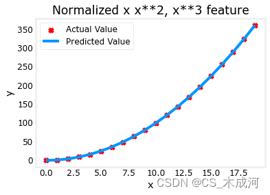
特征缩放使得收敛速度更快。梯度下降过程中, x 2 x^2 x2 是最受强调的, x 3 x^3 x3项几乎被消除。
4. 复杂函数
通过特征工程,甚至可以对相当复杂的函数进行建模:
x = np.arange(0,20,1)
y = np.cos(x/2)X = np.c_[x, x**2, x**3,x**4, x**5, x**6, x**7, x**8, x**9, x**10, x**11, x**12, x**13]
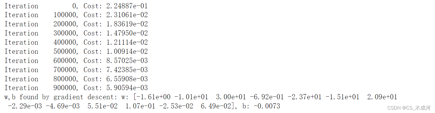
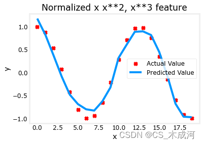
X = zscore_normalize_features(X) model_w,model_b = run_gradient_descent_feng(X, y, iterations=1000000, alpha = 1e-1)plt.scatter(x, y, marker='x', c='r', label="Actual Value"); plt.title("Normalized x x**2, x**3 feature")
plt.plot(x,X@model_w + model_b, label="Predicted Value"); plt.xlabel("x"); plt.ylabel("y"); plt.legend(); plt.show()
附录
lab_utils_multi.py源码:
import numpy as np
import copy
import math
from scipy.stats import norm
import matplotlib.pyplot as plt
from mpl_toolkits.mplot3d import axes3d
from matplotlib.ticker import MaxNLocator
dlblue = '#0096ff'; dlorange = '#FF9300'; dldarkred='#C00000'; dlmagenta='#FF40FF'; dlpurple='#7030A0';
plt.style.use('./deeplearning.mplstyle')def load_data_multi():data = np.loadtxt("data/ex1data2.txt", delimiter=',')X = data[:,:2]y = data[:,2]return X, y##########################################################
# Plotting Routines
##########################################################def plt_house_x(X, y,f_wb=None, ax=None):''' plot house with aXis '''if not ax:fig, ax = plt.subplots(1,1)ax.scatter(X, y, marker='x', c='r', label="Actual Value")ax.set_title("Housing Prices")ax.set_ylabel('Price (in 1000s of dollars)')ax.set_xlabel(f'Size (1000 sqft)')if f_wb is not None:ax.plot(X, f_wb,  c=dlblue, label="Our Prediction")ax.legend()def mk_cost_lines(x,y,w,b, ax):''' makes vertical cost lines'''cstr = "cost = (1/2m)*1000*("ctot = 0label = 'cost for point'for p in zip(x,y):f_wb_p = w*p[0]+bc_p = ((f_wb_p - p[1])**2)/2c_p_txt = c_p/1000ax.vlines(p[0], p[1],f_wb_p, lw=3, color=dlpurple, ls='dotted', label=label)label='' #just onecxy = [p[0], p[1] + (f_wb_p-p[1])/2]ax.annotate(f'{c_p_txt:0.0f}', xy=cxy, xycoords='data',color=dlpurple, xytext=(5, 0), textcoords='offset points')cstr += f"{c_p_txt:0.0f} +"ctot += c_pctot = ctot/(len(x))cstr = cstr[:-1] + f") = {ctot:0.0f}"ax.text(0.15,0.02,cstr, transform=ax.transAxes, color=dlpurple)def inbounds(a,b,xlim,ylim):xlow,xhigh = xlimylow,yhigh = ylimax, ay = abx, by = bif (ax > xlow and ax < xhigh) and (bx > xlow and bx < xhigh) \and (ay > ylow and ay < yhigh) and (by > ylow and by < yhigh):return(True)else:return(False)from mpl_toolkits.mplot3d import axes3d
def plt_contour_wgrad(x, y, hist, ax, w_range=[-100, 500, 5], b_range=[-500, 500, 5], contours = [0.1,50,1000,5000,10000,25000,50000], resolution=5, w_final=200, b_final=100,step=10 ):b0,w0 = np.meshgrid(np.arange(*b_range),np.arange(*w_range))z=np.zeros_like(b0)n,_ = w0.shapefor i in range(w0.shape[0]):for j in range(w0.shape[1]):z[i][j] = compute_cost(x, y, w0[i][j], b0[i][j] )CS = ax.contour(w0, b0, z, contours, linewidths=2,colors=[dlblue, dlorange, dldarkred, dlmagenta, dlpurple]) ax.clabel(CS, inline=1, fmt='%1.0f', fontsize=10)ax.set_xlabel("w");  ax.set_ylabel("b")ax.set_title('Contour plot of cost J(w,b), vs b,w with path of gradient descent')w = w_final; b=b_finalax.hlines(b, ax.get_xlim()[0],w, lw=2, color=dlpurple, ls='dotted')ax.vlines(w, ax.get_ylim()[0],b, lw=2, color=dlpurple, ls='dotted')base = hist[0]for point in hist[0::step]:edist = np.sqrt((base[0] - point[0])**2 + (base[1] - point[1])**2)if(edist > resolution or point==hist[-1]):if inbounds(point,base, ax.get_xlim(),ax.get_ylim()):plt.annotate('', xy=point, xytext=base,xycoords='data',arrowprops={'arrowstyle': '->', 'color': 'r', 'lw': 3},va='center', ha='center')base=pointreturn# plots p1 vs p2. Prange is an array of entries [min, max, steps]. In feature scaling lab.
def plt_contour_multi(x, y, w, b, ax, prange, p1, p2, title="", xlabel="", ylabel=""): contours = [1e2, 2e2,3e2,4e2, 5e2, 6e2, 7e2,8e2,1e3, 1.25e3,1.5e3, 1e4, 1e5, 1e6, 1e7]px,py = np.meshgrid(np.linspace(*(prange[p1])),np.linspace(*(prange[p2])))z=np.zeros_like(px)n,_ = px.shapefor i in range(px.shape[0]):for j in range(px.shape[1]):w_ij = wb_ij = bif p1 <= 3: w_ij[p1] = px[i,j]if p1 == 4: b_ij = px[i,j]if p2 <= 3: w_ij[p2] = py[i,j]if p2 == 4: b_ij = py[i,j]z[i][j] = compute_cost(x, y, w_ij, b_ij )CS = ax.contour(px, py, z, contours, linewidths=2,colors=[dlblue, dlorange, dldarkred, dlmagenta, dlpurple]) ax.clabel(CS, inline=1, fmt='%1.2e', fontsize=10)ax.set_xlabel(xlabel);  ax.set_ylabel(ylabel)ax.set_title(title, fontsize=14)def plt_equal_scale(X_train, X_norm, y_train):fig,ax = plt.subplots(1,2,figsize=(12,5))prange = [[ 0.238-0.045, 0.238+0.045,  50],[-25.77326319-0.045, -25.77326319+0.045, 50],[-50000, 0,      50],[-1500,  0,      50],[0, 200000, 50]]w_best = np.array([0.23844318, -25.77326319, -58.11084634,  -1.57727192])b_best = 235plt_contour_multi(X_train, y_train, w_best, b_best, ax[0], prange, 0, 1, title='Unnormalized, J(w,b), vs w[0],w[1]',xlabel= "w[0] (size(sqft))", ylabel="w[1] (# bedrooms)")#w_best = np.array([111.1972, -16.75480051, -28.51530411, -37.17305735])b_best = 376.949151515151prange = [[ 111-50, 111+50,   75],[-16.75-50,-16.75+50, 75],[-28.5-8, -28.5+8,  50],[-37.1-16,-37.1+16, 50],[376-150, 376+150, 50]]plt_contour_multi(X_norm, y_train, w_best, b_best, ax[1], prange, 0, 1, title='Normalized, J(w,b), vs w[0],w[1]',xlabel= "w[0] (normalized size(sqft))", ylabel="w[1] (normalized # bedrooms)")fig.suptitle("Cost contour with equal scale", fontsize=18)#plt.tight_layout(rect=(0,0,1.05,1.05))fig.tight_layout(rect=(0,0,1,0.95))plt.show()def plt_divergence(p_hist, J_hist, x_train,y_train):x=np.zeros(len(p_hist))y=np.zeros(len(p_hist))v=np.zeros(len(p_hist))for i in range(len(p_hist)):x[i] = p_hist[i][0]y[i] = p_hist[i][1]v[i] = J_hist[i]fig = plt.figure(figsize=(12,5))plt.subplots_adjust( wspace=0 )gs = fig.add_gridspec(1, 5)fig.suptitle(f"Cost escalates when learning rate is too large")#===============#  First subplot#===============ax = fig.add_subplot(gs[:2], )# Print w vs cost to see minimumfix_b = 100w_array = np.arange(-70000, 70000, 1000)cost = np.zeros_like(w_array)for i in range(len(w_array)):tmp_w = w_array[i]cost[i] = compute_cost(x_train, y_train, tmp_w, fix_b)ax.plot(w_array, cost)ax.plot(x,v, c=dlmagenta)ax.set_title("Cost vs w, b set to 100")ax.set_ylabel('Cost')ax.set_xlabel('w')ax.xaxis.set_major_locator(MaxNLocator(2)) #===============# Second Subplot#===============tmp_b,tmp_w = np.meshgrid(np.arange(-35000, 35000, 500),np.arange(-70000, 70000, 500))z=np.zeros_like(tmp_b)for i in range(tmp_w.shape[0]):for j in range(tmp_w.shape[1]):z[i][j] = compute_cost(x_train, y_train, tmp_w[i][j], tmp_b[i][j] )ax = fig.add_subplot(gs[2:], projection='3d')ax.plot_surface(tmp_w, tmp_b, z,  alpha=0.3, color=dlblue)ax.xaxis.set_major_locator(MaxNLocator(2)) ax.yaxis.set_major_locator(MaxNLocator(2)) ax.set_xlabel('w', fontsize=16)ax.set_ylabel('b', fontsize=16)ax.set_zlabel('\ncost', fontsize=16)plt.title('Cost vs (b, w)')# Customize the view angle ax.view_init(elev=20., azim=-65)ax.plot(x, y, v,c=dlmagenta)return# draw derivative line
# y = m*(x - x1) + y1
def add_line(dj_dx, x1, y1, d, ax):x = np.linspace(x1-d, x1+d,50)y = dj_dx*(x - x1) + y1ax.scatter(x1, y1, color=dlblue, s=50)ax.plot(x, y, '--', c=dldarkred,zorder=10, linewidth = 1)xoff = 30 if x1 == 200 else 10ax.annotate(r"$\frac{\partial J}{\partial w}$ =%d" % dj_dx, fontsize=14,xy=(x1, y1), xycoords='data',xytext=(xoff, 10), textcoords='offset points',arrowprops=dict(arrowstyle="->"),horizontalalignment='left', verticalalignment='top')def plt_gradients(x_train,y_train, f_compute_cost, f_compute_gradient):#===============#  First subplot#===============fig,ax = plt.subplots(1,2,figsize=(12,4))# Print w vs cost to see minimumfix_b = 100w_array = np.linspace(-100, 500, 50)w_array = np.linspace(0, 400, 50)cost = np.zeros_like(w_array)for i in range(len(w_array)):tmp_w = w_array[i]cost[i] = f_compute_cost(x_train, y_train, tmp_w, fix_b)ax[0].plot(w_array, cost,linewidth=1)ax[0].set_title("Cost vs w, with gradient; b set to 100")ax[0].set_ylabel('Cost')ax[0].set_xlabel('w')# plot lines for fixed b=100for tmp_w in [100,200,300]:fix_b = 100dj_dw,dj_db = f_compute_gradient(x_train, y_train, tmp_w, fix_b )j = f_compute_cost(x_train, y_train, tmp_w, fix_b)add_line(dj_dw, tmp_w, j, 30, ax[0])#===============# Second Subplot#===============tmp_b,tmp_w = np.meshgrid(np.linspace(-200, 200, 10), np.linspace(-100, 600, 10))U = np.zeros_like(tmp_w)V = np.zeros_like(tmp_b)for i in range(tmp_w.shape[0]):for j in range(tmp_w.shape[1]):U[i][j], V[i][j] = f_compute_gradient(x_train, y_train, tmp_w[i][j], tmp_b[i][j] )X = tmp_wY = tmp_bn=-2color_array = np.sqrt(((V-n)/2)**2 + ((U-n)/2)**2)ax[1].set_title('Gradient shown in quiver plot')Q = ax[1].quiver(X, Y, U, V, color_array, units='width', )qk = ax[1].quiverkey(Q, 0.9, 0.9, 2, r'$2 \frac{m}{s}$', labelpos='E',coordinates='figure')ax[1].set_xlabel("w"); ax[1].set_ylabel("b")def norm_plot(ax, data):scale = (np.max(data) - np.min(data))*0.2x = np.linspace(np.min(data)-scale,np.max(data)+scale,50)_,bins, _ = ax.hist(data, x, color="xkcd:azure")#ax.set_ylabel("Count")mu = np.mean(data); std = np.std(data); dist = norm.pdf(bins, loc=mu, scale = std)axr = ax.twinx()axr.plot(bins,dist, color = "orangered", lw=2)axr.set_ylim(bottom=0)axr.axis('off')def plot_cost_i_w(X,y,hist):ws = np.array([ p[0] for p in hist["params"]])rng = max(abs(ws[:,0].min()),abs(ws[:,0].max()))wr = np.linspace(-rng+0.27,rng+0.27,20)cst = [compute_cost(X,y,np.array([wr[i],-32, -67, -1.46]), 221) for i in range(len(wr))]fig,ax = plt.subplots(1,2,figsize=(12,3))ax[0].plot(hist["iter"], (hist["cost"]));  ax[0].set_title("Cost vs Iteration")ax[0].set_xlabel("iteration"); ax[0].set_ylabel("Cost")ax[1].plot(wr, cst); ax[1].set_title("Cost vs w[0]")ax[1].set_xlabel("w[0]"); ax[1].set_ylabel("Cost")ax[1].plot(ws[:,0],hist["cost"])plt.show()##########################################################
# Regression Routines
##########################################################def compute_gradient_matrix(X, y, w, b): """Computes the gradient for linear regression Args:X : (array_like Shape (m,n)) variable such as house size y : (array_like Shape (m,1)) actual value w : (array_like Shape (n,1)) Values of parameters of the model      b : (scalar )                Values of parameter of the model      Returnsdj_dw: (array_like Shape (n,1)) The gradient of the cost w.r.t. the parameters w. dj_db: (scalar)                The gradient of the cost w.r.t. the parameter b. """m,n = X.shapef_wb = X @ w + b              e   = f_wb - y                dj_dw  = (1/m) * (X.T @ e)    dj_db  = (1/m) * np.sum(e)    return dj_db,dj_dw#Function to calculate the cost
def compute_cost_matrix(X, y, w, b, verbose=False):"""Computes the gradient for linear regression Args:X : (array_like Shape (m,n)) variable such as house size y : (array_like Shape (m,)) actual value w : (array_like Shape (n,)) parameters of the model b : (scalar               ) parameter of the model verbose : (Boolean) If true, print out intermediate value f_wbReturnscost: (scalar)                      """ m,n = X.shape# calculate f_wb for all examples.f_wb = X @ w + b  # calculate costtotal_cost = (1/(2*m)) * np.sum((f_wb-y)**2)if verbose: print("f_wb:")if verbose: print(f_wb)return total_cost# Loop version of multi-variable compute_cost
def compute_cost(X, y, w, b): """compute costArgs:X : (ndarray): Shape (m,n) matrix of examples with multiple featuresw : (ndarray): Shape (n)   parameters for prediction   b : (scalar):              parameter  for prediction   Returnscost: (scalar)             cost"""m = X.shape[0]cost = 0.0for i in range(m):                                f_wb_i = np.dot(X[i],w) + b       cost = cost + (f_wb_i - y[i])**2              cost = cost/(2*m)                                 return(np.squeeze(cost)) def compute_gradient(X, y, w, b): """Computes the gradient for linear regression Args:X : (ndarray Shape (m,n)) matrix of examples y : (ndarray Shape (m,))  target value of each examplew : (ndarray Shape (n,))  parameters of the model      b : (scalar)              parameter of the model      Returnsdj_dw : (ndarray Shape (n,)) The gradient of the cost w.r.t. the parameters w. dj_db : (scalar)             The gradient of the cost w.r.t. the parameter b. """m,n = X.shape           #(number of examples, number of features)dj_dw = np.zeros((n,))dj_db = 0.for i in range(m):                             err = (np.dot(X[i], w) + b) - y[i]   for j in range(n):                         dj_dw[j] = dj_dw[j] + err * X[i,j]    dj_db = dj_db + err                        dj_dw = dj_dw/m                                dj_db = dj_db/m                                return dj_db,dj_dw#This version saves more values and is more verbose than the assigment versons
def gradient_descent_houses(X, y, w_in, b_in, cost_function, gradient_function, alpha, num_iters): """Performs batch gradient descent to learn theta. Updates theta by taking num_iters gradient steps with learning rate alphaArgs:X : (array_like Shape (m,n)    matrix of examples y : (array_like Shape (m,))    target value of each examplew_in : (array_like Shape (n,)) Initial values of parameters of the modelb_in : (scalar)                Initial value of parameter of the modelcost_function: function to compute costgradient_function: function to compute the gradientalpha : (float) Learning ratenum_iters : (int) number of iterations to run gradient descentReturnsw : (array_like Shape (n,)) Updated values of parameters of the model afterrunning gradient descentb : (scalar)                Updated value of parameter of the model afterrunning gradient descent"""# number of training examplesm = len(X)# An array to store values at each iteration primarily for graphing laterhist={}hist["cost"] = []; hist["params"] = []; hist["grads"]=[]; hist["iter"]=[];w = copy.deepcopy(w_in)  #avoid modifying global w within functionb = b_insave_interval = np.ceil(num_iters/10000) # prevent resource exhaustion for long runsprint(f"Iteration Cost          w0       w1       w2       w3       b       djdw0    djdw1    djdw2    djdw3    djdb  ")print(f"---------------------|--------|--------|--------|--------|--------|--------|--------|--------|--------|--------|")for i in range(num_iters):# Calculate the gradient and update the parametersdj_db,dj_dw = gradient_function(X, y, w, b)   # Update Parameters using w, b, alpha and gradientw = w - alpha * dj_dw               b = b - alpha * dj_db               # Save cost J,w,b at each save interval for graphingif i == 0 or i % save_interval == 0:     hist["cost"].append(cost_function(X, y, w, b))hist["params"].append([w,b])hist["grads"].append([dj_dw,dj_db])hist["iter"].append(i)# Print cost every at intervals 10 times or as many iterations if < 10if i% math.ceil(num_iters/10) == 0:#print(f"Iteration {i:4d}: Cost {cost_function(X, y, w, b):8.2f}   ")cst = cost_function(X, y, w, b)print(f"{i:9d} {cst:0.5e} {w[0]: 0.1e} {w[1]: 0.1e} {w[2]: 0.1e} {w[3]: 0.1e} {b: 0.1e} {dj_dw[0]: 0.1e} {dj_dw[1]: 0.1e} {dj_dw[2]: 0.1e} {dj_dw[3]: 0.1e} {dj_db: 0.1e}")return w, b, hist #return w,b and history for graphingdef run_gradient_descent(X,y,iterations=1000, alpha = 1e-6):m,n = X.shape# initialize parametersinitial_w = np.zeros(n)initial_b = 0# run gradient descentw_out, b_out, hist_out = gradient_descent_houses(X ,y, initial_w, initial_b,compute_cost, compute_gradient_matrix, alpha, iterations)print(f"w,b found by gradient descent: w: {w_out}, b: {b_out:0.2f}")return(w_out, b_out, hist_out)# compact extaction of hist data
#x = hist["iter"]
#J  = np.array([ p    for p in hist["cost"]])
#ws = np.array([ p[0] for p in hist["params"]])
#dj_ws = np.array([ p[0] for p in hist["grads"]])#bs = np.array([ p[1] for p in hist["params"]]) def run_gradient_descent_feng(X,y,iterations=1000, alpha = 1e-6):m,n = X.shape# initialize parametersinitial_w = np.zeros(n)initial_b = 0# run gradient descentw_out, b_out, hist_out = gradient_descent(X ,y, initial_w, initial_b,compute_cost, compute_gradient_matrix, alpha, iterations)print(f"w,b found by gradient descent: w: {w_out}, b: {b_out:0.4f}")return(w_out, b_out)def gradient_descent(X, y, w_in, b_in, cost_function, gradient_function, alpha, num_iters): """Performs batch gradient descent to learn theta. Updates theta by taking num_iters gradient steps with learning rate alphaArgs:X : (array_like Shape (m,n)    matrix of examples y : (array_like Shape (m,))    target value of each examplew_in : (array_like Shape (n,)) Initial values of parameters of the modelb_in : (scalar)                Initial value of parameter of the modelcost_function: function to compute costgradient_function: function to compute the gradientalpha : (float) Learning ratenum_iters : (int) number of iterations to run gradient descentReturnsw : (array_like Shape (n,)) Updated values of parameters of the model afterrunning gradient descentb : (scalar)                Updated value of parameter of the model afterrunning gradient descent"""# number of training examplesm = len(X)# An array to store values at each iteration primarily for graphing laterhist={}hist["cost"] = []; hist["params"] = []; hist["grads"]=[]; hist["iter"]=[];w = copy.deepcopy(w_in)  #avoid modifying global w within functionb = b_insave_interval = np.ceil(num_iters/10000) # prevent resource exhaustion for long runsfor i in range(num_iters):# Calculate the gradient and update the parametersdj_db,dj_dw = gradient_function(X, y, w, b)   # Update Parameters using w, b, alpha and gradientw = w - alpha * dj_dw               b = b - alpha * dj_db               # Save cost J,w,b at each save interval for graphingif i == 0 or i % save_interval == 0:     hist["cost"].append(cost_function(X, y, w, b))hist["params"].append([w,b])hist["grads"].append([dj_dw,dj_db])hist["iter"].append(i)# Print cost every at intervals 10 times or as many iterations if < 10if i% math.ceil(num_iters/10) == 0:#print(f"Iteration {i:4d}: Cost {cost_function(X, y, w, b):8.2f}   ")cst = cost_function(X, y, w, b)print(f"Iteration {i:9d}, Cost: {cst:0.5e}")return w, b, hist #return w,b and history for graphingdef load_house_data():data = np.loadtxt("./data/houses.txt", delimiter=',', skiprows=1)X = data[:,:4]y = data[:,4]return X, ydef zscore_normalize_features(X,rtn_ms=False):"""returns z-score normalized X by columnArgs:X : (numpy array (m,n)) ReturnsX_norm: (numpy array (m,n)) input normalized by column"""mu     = np.mean(X,axis=0)  sigma  = np.std(X,axis=0)X_norm = (X - mu)/sigma      if rtn_ms:return(X_norm, mu, sigma)else:return(X_norm)
相关文章:
【机器学习】Feature Engineering and Polynomial Regression
Feature Engineering and Polynomial Regression 1. 多项式特征2. 选择特征3. 缩放特征4. 复杂函数附录 首先,导入所需的库: import numpy as np import matplotlib.pyplot as plt from lab_utils_multi import zscore_normalize_features, run_gradien…...

Rust- 变量绑定
In Rust, you bind values to a variable name using the let keyword. This is often referred to as “variable binding” because it’s like binding a name to a value. Here’s a simple example: let x 5;In this example, x is bound to the value 5. By default, …...
向“数”而“深”,联想凌拓的“破局求变”底气何来?
前言:要赢得更多机遇,“破局求变”尤为重要。 【全球存储观察 | 热点关注】2019年2月25日,承袭联想集团与NetApp的“双基因”,联想凌拓正式成立。历经四年多的发展,联想凌拓已成为中国企业级数据管理领域的…...
pytorch实战-图像分类(二)(模型训练及验证)(基于迁移学习(理解+代码))
目录 1.迁移学习概念 2.数据预处理 3.训练模型(基于迁移学习) 3.1选择网络,这里用resnet 3.2如果用GPU训练,需要加入以下代码 3.3卷积层冻结模块 3.4加载resnet152模 3.5解释initialize_model函数 3.6迁移学习网络搭建 3.…...
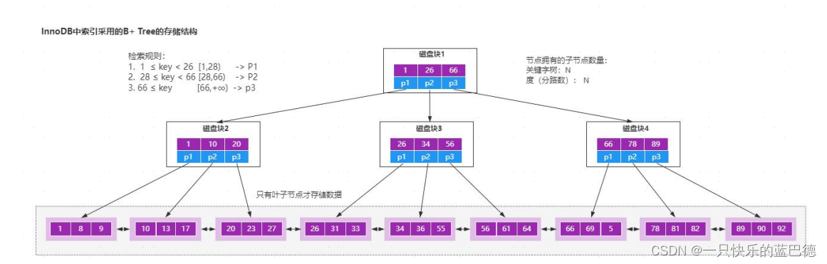
b 树和 b+树的理解
项目场景: 图灵奖获得者(Niklaus Wirth )说过: 程序 数据结构 算法, 也就说我们无时无刻 都在和数据结构打交道。 只是作为 Java 开发,由于技术体系的成熟度较高,使得大部分人认为࿱…...

正则表达式 —— Awk
Awk awk:文本三剑客之一,是功能最强大的文本工具 awk也是按行来进行操作,对行操作完之后,可以根据指定命令来对行取列 awk的分隔符,默认分隔符是空格或tab键,多个空格会压缩成一个 awk的用法 awk的格式…...

国芯新作 | 四核Cortex-A53@1.4GHz,仅168元起?含税?哇!!!
创龙科技SOM-TLT507是一款基于全志科技T507-H处理器设计的4核ARM Cortex-A53全国产工业核心板,主频高达1.416GHz。核心板CPU、ROM、RAM、电源、晶振等所有元器件均采用国产工业级方案,国产化率100%。 核心板通过邮票孔连接方式引出MIPI CSI、HDMI OUT、…...
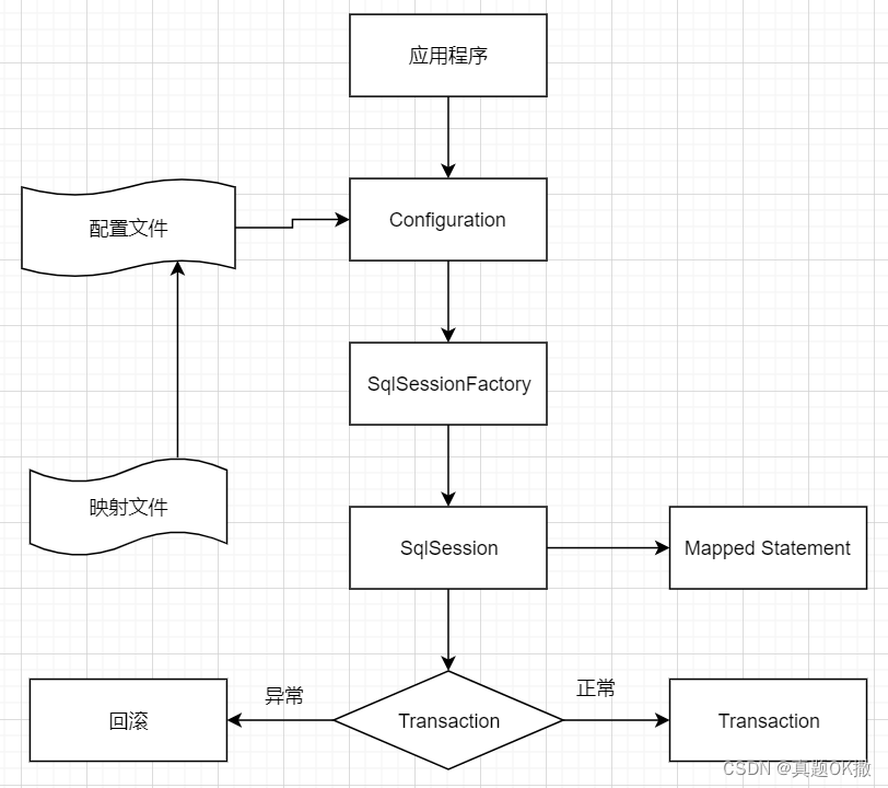
【MyBatis】 框架原理
目录 10.3【MyBatis】 框架原理 10.3.1 【MyBatis】 整体架构 10.3.2 【MyBatis】 运行原理 10.4 【MyBatis】 核心组件的生命周期 10.4.1 SqlSessionFactoryBuilder 10.4.2 SqlSessionFactory 10.4.3 SqlSession 10.4.4 Mapper Instances 与 Hibernate 框架相比&#…...
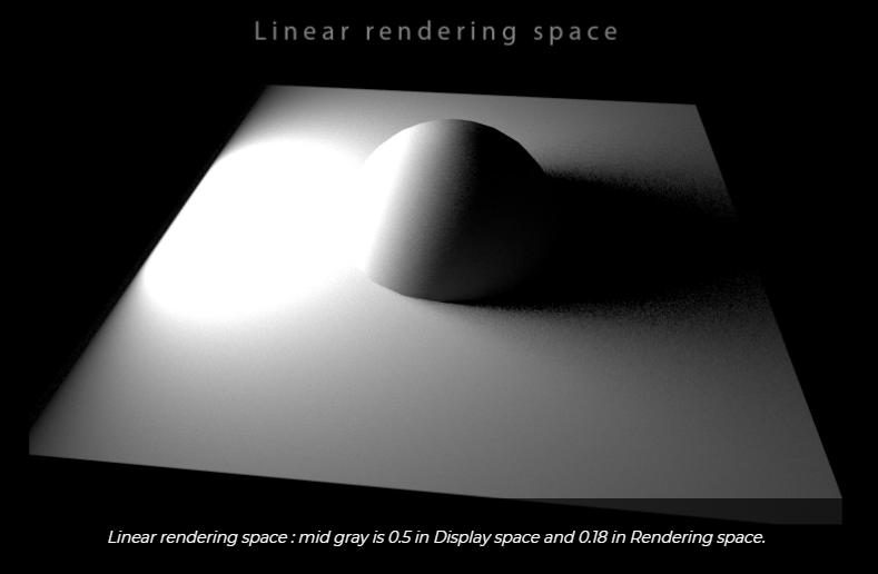
三、线性工作流
再生产的各个环节,正确使用gamma编码及gamma解码,使得最终得到的颜色数据与最初输入的物理数据一致。如果使用gamma空间的贴图,在传给着色器前需要从gamma空间转到线性空间。 如果不在线性空间下进行渲染,会产生的问题:…...
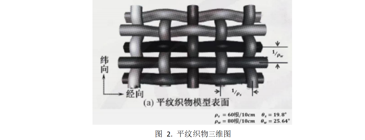
2023华数杯数学建模A题思路 - 隔热材料的结构优化控制研究
# 1 赛题 A 题 隔热材料的结构优化控制研究 新型隔热材料 A 具有优良的隔热特性,在航天、军工、石化、建筑、交通等 高科技领域中有着广泛的应用。 目前,由单根隔热材料 A 纤维编织成的织物,其热导率可以直接测出;但是 单根隔热…...
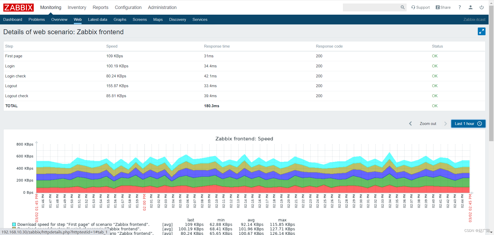
Zabbix分布式监控Web监控
目录 1 概述2 配置 Web 场景2.1 配置步骤2.2 显示 3 Web 场景步骤3.1 创建新的 Web 场景。3.2 定义场景的步骤3.3 保存配置完成的Web 监控场景。 4 Zabbix-Get的使用 1 概述 您可以使用 Zabbix 对多个网站进行可用性方面监控: 要使用 Web 监控,您需要定…...

PHP从入门到精通—PHP开发入门-PHP概述、PHP开发环境搭建、PHP开发环境搭建、第一个PHP程序、PHP开发流程
每开始学习一门语言,都要了解这门语言和进行开发环境的搭建。同样,学生开始PHP学习之前,首先要了解这门语言的历史、语言优势等内容以及了解开发环境的搭建。 PHP概述 认识PHP PHP最初是由Rasmus Lerdorf于1994年为了维护个人网页而编写的一…...

【LeetCode-中等】722. 删除注释
题目链接 722. 删除注释 标签 字符串 步骤 Step1. 先将source合并为一个字符串进行处理,中间补上’\n’,方便后续确定注释开始、结束位置。 string combined; for (auto str : source) {combined str "\n"; }Step2. 定义数组 toDel&am…...

rust里如何判断字符串是否相等呢?
在 Rust 中,有几种方法可以判断字符串是否相等。下面是其中几种常见的方法: 使用 运算符:可以直接使用 运算符比较两个字符串是否相等。例如: fn main() {let str1 "hello";let str2 "world";if str1 …...
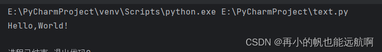
python基本知识学习
一、输出语句 在控制台输出Hello,World! print("Hello,World!") 二、注释 单行注释:以#开头 # print("你好") 多行注释: 选中要注释的代码Ctrl/三单引号三双引号 # print("你好") # a1 # a2 print("Hello,World!&…...
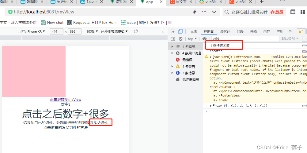
vue3和typescript_组件
1 components下新建myComponent.vue 2 页面中引入组件,传入值,并且绑定事件函数。 3...

Qt+联想电脑管家
1.自定义按钮类 效果: (1)仅当未选中,未悬浮时 (2)其他三种情况,均如图 #ifndef BTN_H #define BTN_H#include <QPushButton> class btn : public QPushButton {Q_OBJECT public:btn(QWidget * parent nullptr);void set_normal_icon(…...
论文阅读-BotPercent: Estimating Twitter Bot Populations from Groups to Crowds
目录 摘要 引言 方法 数据集 BotPercent架构 实验结果 活跃用户中的Bot数量 Bot Population among Comment Sections Bot Participation in Content Moderation Votes Bot Population in Different Countries’ Politics 论文链接:https://arxiv.org/pdf/23…...
用于永磁同步电机驱动器的自适应SDRE非线性无传感器速度控制(MatlabSimulink实现)
💥💥💞💞欢迎来到本博客❤️❤️💥💥 🏆博主优势:🌞🌞🌞博客内容尽量做到思维缜密,逻辑清晰,为了方便读者。 ⛳️座右铭&a…...

Spring Cloud+Spring Boot+Mybatis+uniapp+前后端分离实现知识付费平台免费搭建 qt
Java版知识付费源码 Spring CloudSpring BootMybatisuniapp前后端分离实现知识付费平台 提供职业教育、企业培训、知识付费系统搭建服务。系统功能包含:录播课、直播课、题库、营销、公司组织架构、员工入职培训等。 提供私有化部署,免费售…...
)
给Python异步代码加上类型提示(Type Hints)
为Python异步代码添加类型提示:提升健壮性与可维护性 在Python生态中,异步编程(asyncio)已成为处理高并发场景的核心工具,但动态类型的特性使得代码在复杂项目中容易变得难以维护。通过引入类型提示(Type …...

g4f提供的模型调用:python JavaScript和curl
g4f提供模型的使用,例子页面:G4F - Providers and Models 可以这样: python from g4f.client import Clientclient Client() response client.chat.completions.create(model"",messages[{"role": "user"…...

Context Engineering:比Prompt Engineering更重要的AI任务构建秘籍!
Context Engineering是一门设计和构建动态系统的学科,旨在为LLM提供适时、适格、适切的信息和工具,以高效完成任务。它与Prompt Engineering的区别在于,后者关注提示词编写,前者则侧重完整的信息供给系统构建。Context Engineerin…...

Flutter APK打包遇阻:深入剖析‘gen_snapshot’缺失引发的非零退出值错误
1. 问题现象:Flutter打包APK时遭遇的"拦路虎" 最近在Windows系统上用Flutter打包APK时,突然遇到了一个让人头疼的错误。执行flutter build apk命令后,控制台抛出一堆红色错误信息,最显眼的就是那句"Process finish…...

STM32 串口 FIFO 与 DMA 高效数据流设计
1. 为什么需要FIFODMA的串口方案 第一次用STM32做串口通信时,我天真地以为直接调用HAL_UART_Receive_IT()就能搞定所有问题。结果在工业现场调试时,当传感器以115200波特率连续发送数据时,系统直接卡死——这就是典型的数据淹没问题。后来发现…...

Dev-C++ 6.3与5.11版本对比:如何根据你的Windows系统选择最佳IDE版本
Dev-C 6.3与5.11版本深度对比:如何为你的Windows系统选择最佳开发环境 当你在Windows系统上寻找一款轻量级C/C集成开发环境时,Dev-C总是会出现在推荐列表中。但面对Embarcadero Dev-C 6.3和经典的Dev-Cpp 5.11两个主要版本,很多开发者都会陷入…...

应对2026检测新规:论文如何优化?实测10款降低AI率工具,SCI/工科适用
现在写论文最怕的,已经不是查重了。怕什么?怕那个AIGC率太高。 真的,越来越多学校开始抓AIGC检测报告了,重复率放一边,就看你AI痕迹多不多。我自己就是刚爬出坑的25届学姐,这坑我踩得死死的。怎么说呢&…...

保姆级教程:用Python和GEE Python API把本地训练的袋装决策树模型部署到Google Earth Engine
从零部署袋装决策树模型到Google Earth Engine的完整实践指南 当我们需要处理海量遥感数据时,本地计算资源往往捉襟见肘。Google Earth Engine(GEE)提供了强大的云端计算能力,但其原生支持的机器学习算法有限。本文将带你完整实现…...

ESP32-WROVER-E/IE模组硬件选型与外围电路设计实战
1. ESP32-WROVER-E与ESP32-WROVER-IE模组选型指南 第一次接触ESP32-WROVER系列模组时,很多人会被型号后缀搞晕。其实区分E和IE版本只需要记住一个关键点:字母"I"代表外部天线接口。ESP32-WROVER-IE模组预留了IPEX天线座,而ESP32-WR…...
:软件篇之系统工程详解(上篇))
计算机系统基础知识(十七):软件篇之系统工程详解(上篇)
📝 前言 在系统架构设计师的知识体系中,我们学过处理器、存储器、网络协议、数据库、操作系统等具体的计算机技术。但将这些技术组件有效组织起来,设计出一个满足业务需求的完整系统,还需要一套更高层次的思维方式——系统工程。…...