matplotlib绘制三维图
目录
- 线状堆积图 PolygonPlot
- 三维表面图 SurfacePlot
- 散点图ScatterPlot
- 柱形图 BarPlot
- 三维直方图
- 螺旋曲线图 LinePlot
- ContourPlot
- 轮廓图
- 网状图 WireframePlot
- 箭头图
- 二维三维合并
- 文本图Text
- 三维多个子图
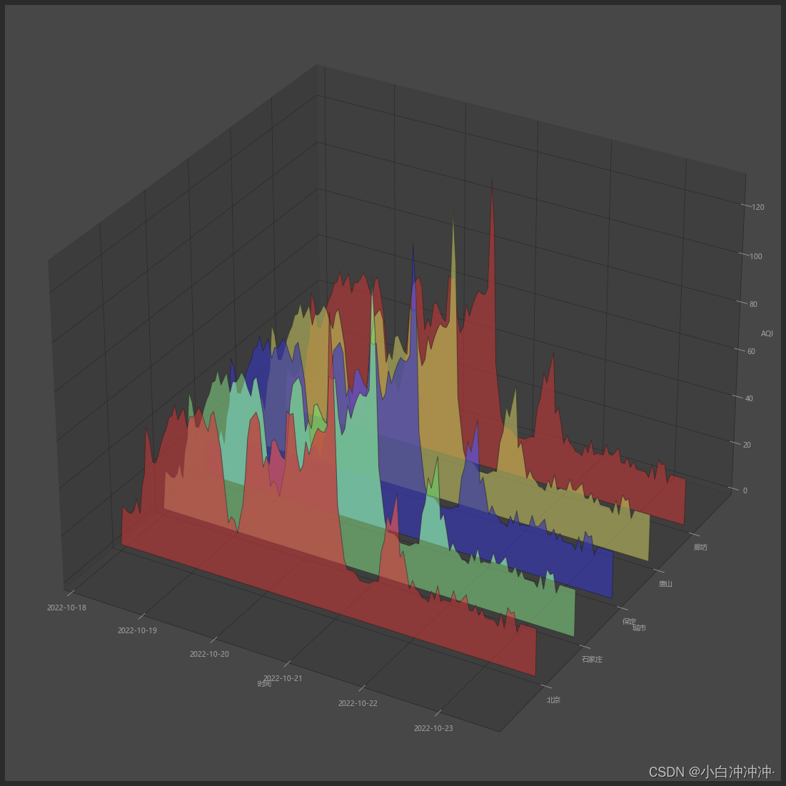
线状堆积图 PolygonPlot
Axes3D.add_collection3d(col, zs=0, zdir=‘z’)
这个函数可以将三维 collection对象或二维collection对象加入到一个图形中,包括:
- PolyCollection
- LineCollection
- PatchCollection
import pandas as pd
from mpl_toolkits.mplot3d import Axes3D
from matplotlib.collections import PolyCollection
import matplotlib.pyplot as plt
from matplotlib import colors as mcolors
import numpy as np
plt.rcParams['font.family'] = 'Microsoft YaHei' # 字体设置
plt.rcParams['font.size'] = 10 # 字体大小设置fig = plt.figure(figsize=(30,20))
ax = fig.gca(projection='3d')def cc(arg):return mcolors.to_rgba(arg, alpha=0.6)
def polygon_under_graph(xlist, ylist):'''Construct the vertex list which defines the polygon filling the space underthe (xlist, ylist) line graph.  Assumes the xs are in ascending order.'''return [(xlist[0], 0.), *zip(xlist, ylist), (xlist[-1], 0.)]xs = np.arange(0,137,1)verts = []zs = [0.0,1.0,2.0, 3.0,4.0]
for z in zs:for i in range(1,6):   #读取数据ys = df.iloc[:,i]verts.append(polygon_under_graph(xs,ys))poly = PolyCollection(verts, facecolors=[cc('r'), cc('g'), cc('b'),cc('y'),cc('r')])
poly.set_alpha(0.7)  # 图形的透明度
ax.add_collection3d(poly, zs=zs, zdir='y')names_1 = ['2022-10-18', '2022-10-19', '2022-10-20','2022-10-21',
'2022-10-22', '2022-10-23']
plt.xticks(xs[::24], names_1)names = ['北京', '石家庄', '保定','唐山','廊坊']
plt.yticks(zs, names)ax.set_xlabel('时间')
ax.set_ylabel('城市')
ax.set_zlabel('AQI')
ax.set_xlim3d(0, 136)
ax.set_ylim3d(-1, 5)
ax.set_zlim3d(0, 130)
#plt.savefig('三维时间.png',bbox_inches = 'tight',dpi=500)
plt.show()
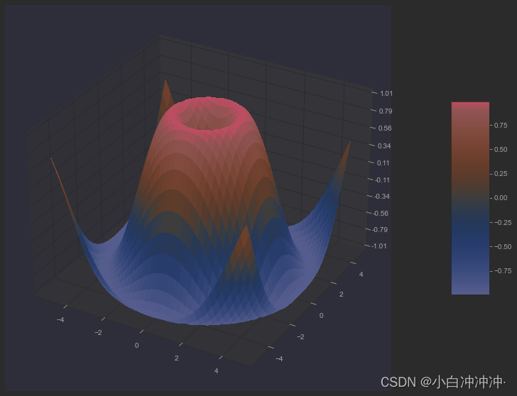
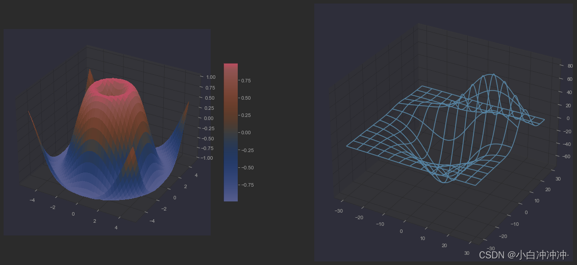
三维表面图 SurfacePlot
Axes3D.plot_surface(X, Y, Z, *args, norm=None, vmin=None, vmax=None, lightsource=None, **kwargs)
这个函数算是比较常用的函数,用于绘制三维表面图,让人惊艳的是它的着色效果。
| Argument | Description |
|---|---|
| X, Y,Z | 坐标点 |
| rcount,ccount,rstride,cstride | 同上 |
| color | 定义surface patch的颜色,type:color-like |
| cmap | 定义surface patch的颜色,只不过是colorMap,type:colormap |
| facecolors | 指定单个patch的颜色, type:array-like of colors |
| norm | colormap的normalization, type:Normalize |
| shade | 阴影效果,type:boolean |
| vmin, vmax | normalization的边界 |
| **kwargs | 向下传递到Poly3DCollection |
| antialiased | 抗锯齿,type:boolean |
from mpl_toolkits.mplot3d import Axes3D
import matplotlib.pyplot as plt
from matplotlib import cmfrom matplotlib.ticker import LinearLocator, FormatStrFormatter
import numpy as npfig = plt.figure(figsize=(30,10))
ax = fig.gca(projection='3d')# Make data.
X = np.arange(-5, 5, 0.25)
Y = np.arange(-5, 5, 0.25)
X, Y = np.meshgrid(X, Y)
R = np.sqrt(X**2 + Y**2)
Z = np.sin(R)# Plot the surface.
surf = ax.plot_surface(X, Y, Z, cmap=cm.coolwarm,linewidth=0, antialiased=False)# Customize the z axis.
ax.set_zlim(-1.01, 1.01)
ax.zaxis.set_major_locator(LinearLocator(10))
ax.zaxis.set_major_formatter(FormatStrFormatter('%.02f'))# Add a color bar which maps values to colors.
fig.colorbar(surf, shrink=0.5, aspect=5)plt.show()
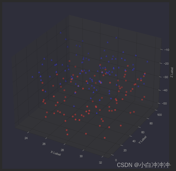
散点图ScatterPlot
Axes3D.scatter(xs, ys, zs=0, zdir=‘z’, s=20, c=None, depthshade=True, *args, **kwargs)
返回Patch3DCollection,
其他参数向下传递给plot函数
| Argument | Description |
|---|---|
| xs, ys | x,y坐标点 |
| zs | z 坐标,可以是一个标量或一个x*y维矩阵,默认是0. |
| zdir | 当绘制二维图像时的z轴方向 |
| s | size,即散点大小 |
| c | 颜色映射,其取值可以是非常多类型,有时间专门写一篇讲解 |
| depthshade | 是否渲染景深(或则就说阴影吧),默认是True. |
from mpl_toolkits.mplot3d import Axes3Dimport matplotlib.pyplot as plt
import numpy as np# Fixing random state for reproducibility
np.random.seed(19680801)def randrange(n, vmin, vmax):'''Helper function to make an array of random numbers having shape (n, )with each number distributed Uniform(vmin, vmax).'''return (vmax - vmin)*np.random.rand(n) + vminfig = plt.figure(figsize=(20,10))
ax = fig.add_subplot(111, projection='3d')n = 100# For each set of style and range settings, plot n random points in the box
# defined by x in [23, 32], y in [0, 100], z in [zlow, zhigh].
for c, m, zlow, zhigh in [('r', 'o', -50, -25), ('b', '^', -30, -5)]:xs = randrange(n, 23, 32)ys = randrange(n, 0, 100)zs = randrange(n, zlow, zhigh)ax.scatter(xs, ys, zs, c=c, marker=m)ax.set_xlabel('X Label')
ax.set_ylabel('Y Label')
ax.set_zlabel('Z Label')plt.show()
柱形图 BarPlot
Axes3D.bar(left, height, zs=0, zdir=‘z’, *args, **kwargs)
其他参数向下传递给bar函数,返回Patch3DCollection对象
| Argument | Description |
|---|---|
| left | 条形图水平坐标 |
| height | 条形的高度 |
| zs | Z方向 |
| zdir | 同上 |
from mpl_toolkits.mplot3d import Axes3D  # noqa: F401 unused importimport matplotlib.pyplot as plt
import numpy as np# Fixing random state for reproducibility
np.random.seed(19680801)fig = plt.figure(figsize=(10,20))
ax = fig.add_subplot(111, projection='3d')colors = ['r', 'g', 'b', 'y']
yticks = [3, 2, 1, 0]
for c, k in zip(colors, yticks):# Generate the random data for the y=k 'layer'.xs = np.arange(20)ys = np.random.rand(20)# You can provide either a single color or an array with the same length as# xs and ys. To demonstrate this, we color the first bar of each set cyan.cs = [c] * len(xs)# Plot the bar graph given by xs and ys on the plane y=k with 80% opacity.ax.bar(xs, ys, zs=k, zdir='y', color=cs, alpha=0.8)ax.set_xlabel('X')
ax.set_ylabel('Y')
ax.set_zlabel('Z')# On the y axis let's only label the discrete values that we have data for.
ax.set_yticks(yticks)plt.show()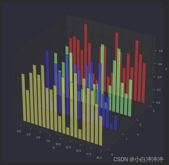
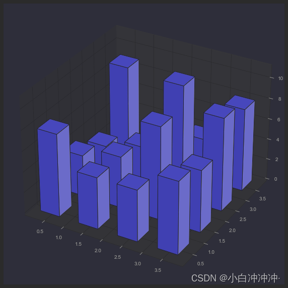
三维直方图
from mpl_toolkits.mplot3d import Axes3D
import matplotlib.pyplot as plt
import numpy as npfig = plt.figure()
ax = fig.add_subplot(111, projection='3d')
x, y = np.random.rand(2, 100) * 4
hist, xedges, yedges = np.histogram2d(x, y, bins=4, range=[[0, 4], [0, 4]])# Construct arrays for the anchor positions of the 16 bars.
# Note: np.meshgrid gives arrays in (ny, nx) so we use 'F' to flatten xpos,
# ypos in column-major order. For numpy >= 1.7, we could instead call meshgrid
# with indexing='ij'.
xpos, ypos = np.meshgrid(xedges[:-1] + 0.25, yedges[:-1] + 0.25)
xpos = xpos.flatten('F')
ypos = ypos.flatten('F')
zpos = np.zeros_like(xpos)# Construct arrays with the dimensions for the 16 bars.
dx = 0.5 * np.ones_like(zpos)
dy = dx.copy()
dz = hist.flatten()ax.bar3d(xpos, ypos, zpos, dx, dy, dz, color='b', zsort='average')plt.show()
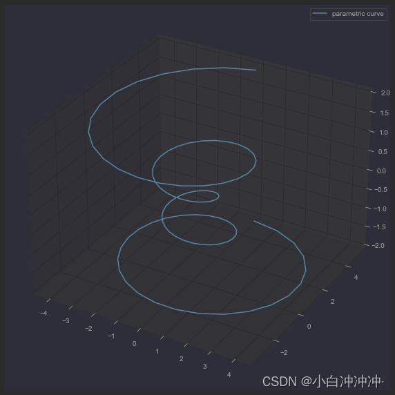
螺旋曲线图 LinePlot
Axes3D.plot(xs, ys, *args, zdir=‘z’, **kwargs)
其他参数向下传递给plot函数
| Argument | Description |
|---|---|
| xs, ys | x、y 坐标 |
| zs | z 坐标,可以是一个标量或一个x*y维矩阵 |
| zdir | 当绘制二维图像时的z轴方向 |
from mpl_toolkits.mplot3d import Axes3Dimport numpy as np
import matplotlib.pyplot as pltplt.rcParams['legend.fontsize'] = 10
fig = plt.figure(figsize=(10,20))
ax = fig.gca(projection='3d')  # get current axes# Prepare arrays x, y, z
theta = np.linspace(-4 * np.pi, 4 * np.pi, 100)
z = np.linspace(-2, 2, 100)
r = z**2 + 1
x = r * np.sin(theta)
y = r * np.cos(theta)ax.plot(x, y, z, label='parametric curve')
ax.legend()  plt.show()
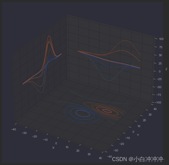
ContourPlot
Axes3D.contour(X, Y, Z, *args, extend3d=False, stride=5, zdir=‘z’, offset=None, **kwargs)
| Argument | Description |
|---|---|
| X, Y,Z | Data values as numpy.arrays |
| extend3d | 是否延申到3d空间 (default: False) |
| *stride | (extend3d的)采样步长 |
| zdir | 同上 |
| offset | 绘制轮廓线在zdir垂直的水平面上的投影 |
from mpl_toolkits.mplot3d import axes3d
import matplotlib.pyplot as plt
from matplotlib import cmfig = plt.figure(figsize=(30,10))
ax = fig.gca(projection='3d')
X, Y, Z = axes3d.get_test_data(0.05)# Plot contour curves
cset = ax.contour(X, Y, Z, cmap=cm.coolwarm)ax.clabel(cset, fontsize=9, inline=1)  # function to label a contourplt.show()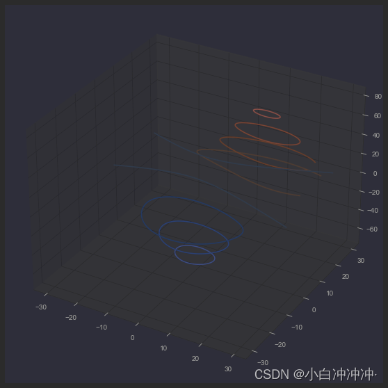
轮廓图
from mpl_toolkits.mplot3d import axes3d
import matplotlib.pyplot as plt
from matplotlib import cmfig = plt.figure()
ax = fig.gca(projection='3d')
X, Y, Z = axes3d.get_test_data(0.05)
cset = ax.contour(X, Y, Z, zdir='z', offset=-100, cmap=cm.coolwarm)
cset = ax.contour(X, Y, Z, zdir='x', offset=-40, cmap=cm.coolwarm)
cset = ax.contour(X, Y, Z, zdir='y', offset=40, cmap=cm.coolwarm)ax.set_xlabel('X')
ax.set_xlim(-40, 40)
ax.set_ylabel('Y')
ax.set_ylim(-40, 40)
ax.set_zlabel('Z')
ax.set_zlim(-100, 100)plt.show()
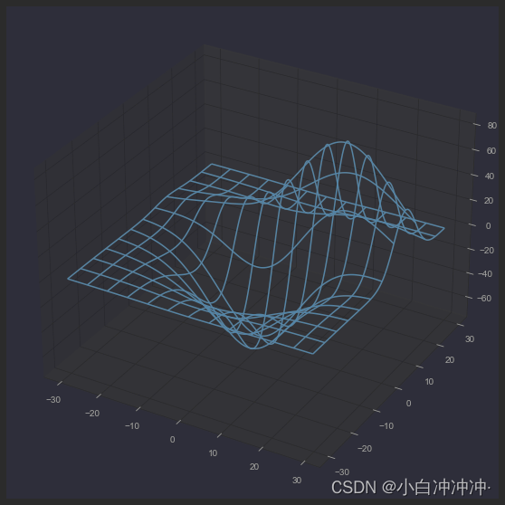
网状图 WireframePlot
Axes3D.plot_wireframe(X, Y, Z, *args, **kwargs)
| Argument | Description |
|---|---|
| X, Y,Z | 坐标点 |
| rcount,ccount | 采样数,越大采样越多,默认50 |
| rstride,cstride | 采样步长,越小采样越多 |
| **kwargs | 其他参数向下传入Line3DCollection |
from mpl_toolkits.mplot3d import axes3d
import matplotlib.pyplot as pltfig = plt.figure(figsize=(30,10))
ax = fig.add_subplot(111, projection='3d')# Grab some test data.
X, Y, Z = axes3d.get_test_data(0.05)# Plot a basic wireframe.
ax.plot_wireframe(X, Y, Z, rstride=10, cstride=10)plt.show()
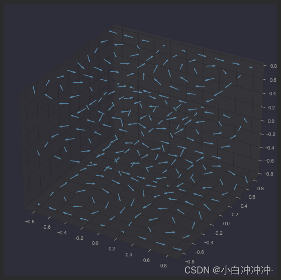
箭头图
Axes3D.quiver(*args, **kwargs)
| Argument | Description |
|---|---|
| X, Y, Z | The x, y and z coordinates of the arrow locations (default is tail of arrow; see pivot kwarg) |
| U, V, W | The x, y and z components of the arrow vectors |
from mpl_toolkits.mplot3d import axes3d
import matplotlib.pyplot as plt
import numpy as npfig = plt.figure()
ax = fig.gca(projection='3d')# Make the grid
x, y, z = np.meshgrid(np.arange(-0.8, 1, 0.2),np.arange(-0.8, 1, 0.2),np.arange(-0.8, 1, 0.8))# Make the direction data for the arrows
u = np.sin(np.pi * x) * np.cos(np.pi * y) * np.cos(np.pi * z)
v = -np.cos(np.pi * x) * np.sin(np.pi * y) * np.cos(np.pi * z)
w = (np.sqrt(2.0 / 3.0) * np.cos(np.pi * x) * np.cos(np.pi * y) *np.sin(np.pi * z))ax.quiver(x, y, z, u, v, w, length=0.1, normalize=True)plt.show()
二维三维合并
from mpl_toolkits.mplot3d import Axes3D
import numpy as np
import matplotlib.pyplot as pltfig = plt.figure()
ax = fig.gca(projection='3d')# Plot a sin curve using the x and y axes.
x = np.linspace(0, 1, 100)
y = np.sin(x * 2 * np.pi) / 2 + 0.5
ax.plot(x, y, zs=0, zdir='z', label='curve in (x,y)')# Plot scatterplot data (20 2D points per colour) on the x and z axes.
colors = ('r', 'g', 'b', 'k')
x = np.random.sample(20 * len(colors))
y = np.random.sample(20 * len(colors))
labels = np.random.randint(3, size=80)# By using zdir='y', the y value of these points is fixed to the zs value 0
# and the (x,y) points are plotted on the x and z axes.
ax.scatter(x, y, zs=0, zdir='y', c=labels, label='points in (x,z)')# Make legend, set axes limits and labels
ax.legend()
ax.set_xlim(0, 1)
ax.set_ylim(0, 1)
ax.set_zlim(0, 1)
ax.set_xlabel('X')
ax.set_ylabel('Y')
ax.set_zlabel('Z')# Customize the view angle so it's easier to see that the scatter points lie
# on the plane y=0
ax.view_init(elev=20., azim=-35)plt.show()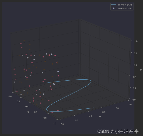
文本图Text
Axes3D.text(x, y, z, s, zdir=None, **kwargs)
text的内容其实也很繁杂,需要用一篇内容去探讨,在三维中很重要的一点是要学会二维、三维文字的添加。
from mpl_toolkits.mplot3d import Axes3D  # noqa: F401 unused importimport matplotlib.pyplot as pltfig = plt.figure()
ax = fig.gca(projection='3d')# Demo 1: zdir
zdirs = (None, 'x', 'y', 'z', (1, 1, 0), (1, 1, 1))
xs = (1, 4, 4, 9, 4, 1)
ys = (2, 5, 8, 10, 1, 2)
zs = (10, 3, 8, 9, 1, 8)for zdir, x, y, z in zip(zdirs, xs, ys, zs):label = '(%d, %d, %d), dir=%s' % (x, y, z, zdir)ax.text(x, y, z, label, zdir)# Demo 2: color
ax.text(9, 0, 0, "red", color='red')# Demo 3: text2D
# Placement 0, 0 would be the bottom left, 1, 1 would be the top right.
ax.text2D(0.05, 0.95, "2D Text", transform=ax.transAxes)# Tweaking display region and labels
ax.set_xlim(0, 10)
ax.set_ylim(0, 10)
ax.set_zlim(0, 10)
ax.set_xlabel('X axis')
ax.set_ylabel('Y axis')
ax.set_zlabel('Z axis')plt.show()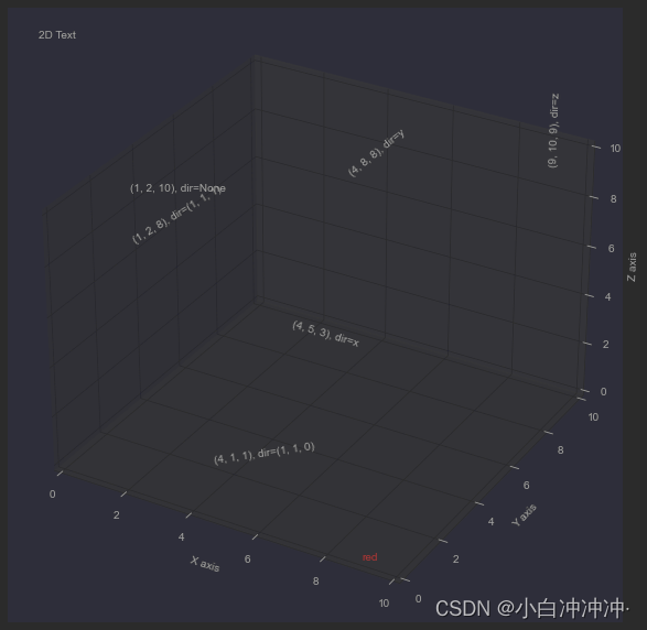
三维多个子图
import matplotlib.pyplot as plt
from mpl_toolkits.mplot3d.axes3d import Axes3D, get_test_data
from matplotlib import cm
import numpy as np# set up a figure twice as wide as it is tall
# fig = plt.figure(figsize=plt.figaspect(0.5))
fig = plt.figure(figsize=(20,10))# ===============
#  First subplot
# ===============
# set up the axes for the first plot
ax = fig.add_subplot(1, 2, 1, projection='3d')# plot a 3D surface like in the example mplot3d/surface3d_demo
X = np.arange(-5, 5, 0.25)
Y = np.arange(-5, 5, 0.25)
X, Y = np.meshgrid(X, Y)
R = np.sqrt(X ** 2 + Y ** 2)
Z = np.sin(R)
surf = ax.plot_surface(X, Y, Z, rstride=1, cstride=1, cmap=cm.coolwarm,linewidth=0, antialiased=False)
ax.set_zlim(-1.01, 1.01)
fig.colorbar(surf, shrink=0.5, aspect=10)# ===============
# Second subplot
# ===============
# set up the axes for the second plot
ax = fig.add_subplot(1, 2, 2, projection='3d')# plot a 3D wireframe like in the example mplot3d/wire3d_demo
X, Y, Z = get_test_data(0.05)
ax.plot_wireframe(X, Y, Z, rstride=10, cstride=10)plt.show()
相关文章:
matplotlib绘制三维图
目录线状堆积图 PolygonPlot三维表面图 SurfacePlot散点图ScatterPlot柱形图 BarPlot三维直方图螺旋曲线图 LinePlotContourPlot轮廓图网状图 WireframePlot箭头图二维三维合并文本图Text三维多个子图线状堆积图 PolygonPlot Axes3D.add_collection3d(col, zs0, zdir‘z’) …...
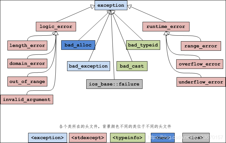
4万字c++讲解+区分c和c++,不来可惜了(含代码+解析)
目录 1 C简介 1.1 起源 1.2 应用范围 1.3 C和C 2开发工具 3 基本语法 3.1 注释 3.2关键字 3.3标识符 4 数据类型 4.1基本数据类型 4.2 数据类型在不同系统中所占空间大小 4.3 typedef声明 4.4 枚举类型 5 变量 5.1 变量的声明和定义 5.2 变量的作用域 6 运算符…...

AcWing 482. 合唱队形
482. 合唱队形N 位同学站成一排,音乐老师要请其中的 (N−K) 位同学出列,使得剩下的 K 位同学排成合唱队形。 合唱队形是指这样的一种队形:设 K位同学从左到右依次编号为 1,2…,K,他们的身高分别为…...
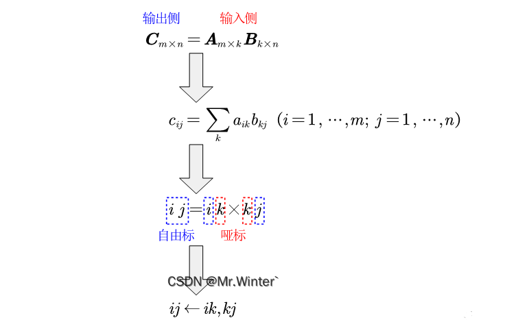
Pytorch深度学习实战3-4:通俗理解张量Tensor的爱因斯坦求和(附实例)
目录1 爱因斯坦求和由来2 爱因斯坦求和原理3 实例:字母表示法3.1 向量运算3.2 矩阵运算3.3 张量运算4 实例:常量表示法4.1 向量运算4.2 矩阵运算4.3 张量运算1 爱因斯坦求和由来 爱因斯坦求和约定(Einstein summation convention)是一种标记的约定&#…...

GEE学习笔记 五十六:GEE中如何把文件导出到Google Drive的子目录
今天在群里看到有人在问一个问题,如何使用GEE把文件导出到Google Drive的子目录中?这里我就简单的说一下这个问题。 首先,在GEE中我们都知道了如何将数据导出导出Google Drive的文件夹中,如下面的一个例子: var geome…...

【Go基础】数据库编程
文章目录1. SQL语法简介2. MySQL最佳实践3. Go SQL驱动接口解读4. 数据库增删改查5. stmt6. SQLBuilder6.1 Go-SQLBuilder6.2 Gendry6.3 自行实现SQLBuilder7. GORM8. Go操作MongoDB1. SQL语法简介 SQL(Structured Query Language)是一套语法标准&#…...

【颠覆软件开发】华为自研IDE!未来IDE将不可预测!
IDE是软件开发生态的入口,但目前我们所使用的IDE基本都是由国外巨头提供,比如Visual Studio、Eclipse、JetBrains。这些IDE具有很高的断供风险,与操作系统、芯片、编程语言一样,非常重要。 随着越来越多的软件开始采用云上开发模…...

怎样从零基础学黑客
可以说想学黑客技术,要求你首先是一个“T”字型人才,也就是说电脑的所有领域你都能做的来,而且有一项是精通的。因此作为一个零基础的黑客爱好者来说,没有良好的基础是绝对不行的,下面我就针对想真正学习黑客的零基础朋…...
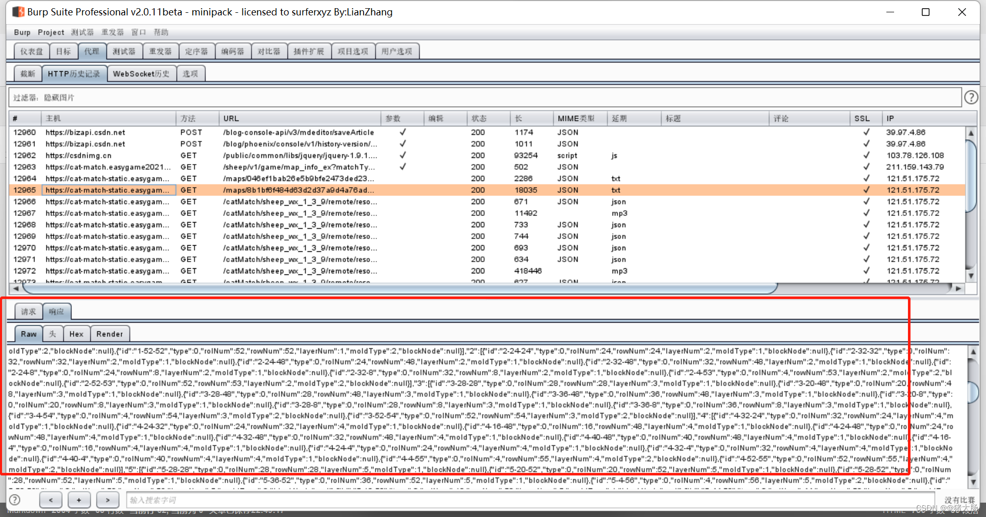
burp小程序抓包
身为一名码农,抓包肯定是一项必备技能。工作中遇到很多次需要对小程序进行抓包排查问题。下面分享一下我的抓包方式,使用的是电脑版小程序抓包,跟手机的方式都差不多的。 一、环境 微信版本:3.6.0.18 Burpsuite版本:…...

文件上传攻击骚操作
允许直接上传shell 只要有文件上传功能,那么就可以尝试上传webshell直接执行恶意代码,获得服务器权限,这是最简单也是最直接的利用。 允许上传压缩包 如果可以上传压缩包,并且服务端会对压缩包解压,那么就可能存在Zip …...
Scala流程控制(第四章:分支控制、嵌套分支、switch分支、for循环控制全、while与do~while、多重与中断)
文章目录第 4 章 流程控制4.1 分支控制 if-else4.1.1 单分支4.1.2 双分支4.1.3 多分支4.2 嵌套分支4.3 Switch 分支结构4.4 For 循环控制4.4.1 范围数据循环(To)4.4.2 范围数据循环(Until)4.4.3 循环守卫4.4.4 循环步长4.4.5 嵌套…...
)
华为OD机试真题Python实现【整理扑克牌】真题+解题思路+代码(20222023)
整理扑克牌 题目 给定一组数字,表示扑克牌的牌面数字,忽略扑克牌的花色,请安如下规则对这一组扑克牌进行整理。 步骤一: 对扑克牌进行分组,规则如下 当牌面数字相同张数大于等于4时,组合牌为炸弹;三张相同牌面数字+两张相同牌面数字,且三张牌与两张牌不相同时,组合牌…...
【春秋云境】CVE-2022-28525
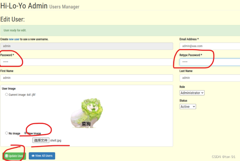
靶标介绍: ED01-CMS v20180505 存在任意文件上传漏洞 打开靶场: 盲猜一波弱密码admin:admin就进去了。登录后在图中位置点击进行图片更新,需要将密码等都写上 抓包将图片信息进行替换,并修改文件名: POST /admin…...

Android设置取消系统闹钟
系统闹钟包名:com.android.deskclock 调用系统闹钟,首先在清单文件AndroidManifest.xml中添加权限: <uses-permission android:name"com.android.alarm.permission.SET_ALARM" />设置系统闹钟: public static v…...

使用 Node.js 多进程提高任务执行效率
什么是 Node 多进程? Node 是在单个线程中运行,我们虽然没办法开启额外的线程,但是可以开启进程集群。这样可以让下载任务和上传任务同时进行。 使用多进程进行初步代码优化 const dl require(./download.js) const ul require(./upload…...
[Golang实战]github.io部署个人博客hugo[新手开箱可用][小白教程]
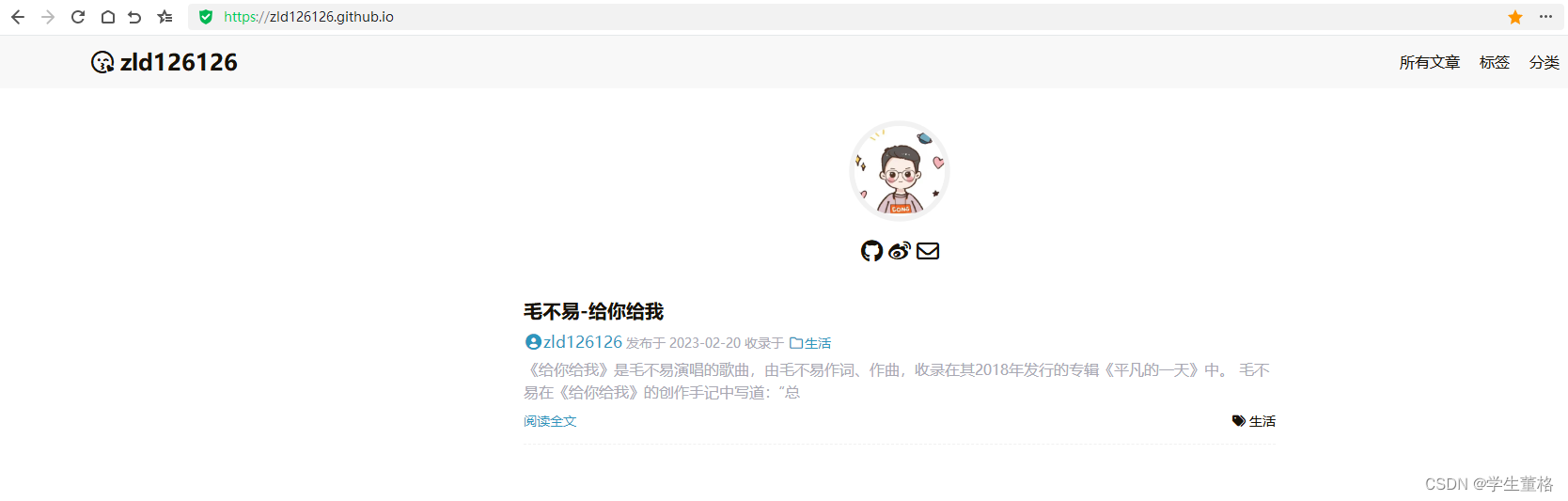
[Golang实战]github.io部署个人博客hugo[新手开箱可用][小白教程]1.新手教程(小白也能学会)2.开始准备2.1myBlog是hugo的项目1.安装Hugo2.创建hugo项目2.2 xxxx.github.io是github.io中规定的pages项目3.成功部署4.TODO自动化workflows部署github.io1.新手教程(小白也能学会) …...

50个 Pandas 高频操作技巧,建议收藏
在数据分析和数据建模的过程中需要对数据进行清洗和整理等工作,有时需要对数据增删字段。 下面为大家介绍Pandas对数据的复杂查询、数据类型转换、数据排序、数据的修改、数据迭代以及函数的使用 文章目录技术交流01、复杂查询1、逻辑运算2、逻辑筛选数据3、函数筛…...

pygraphviz安装教程
0x01. 背景 最近在做casual inference,做实验时候想因果图可视化,遂需要安装pygraphviz,整了一下午,终于捣鼓好了,真头大。 环境: win10操作系统python3.9环境 0x02. 安装Graphviz 传送门:…...

HarmonyOS Connect认证测试
在HarmonyOS Connect生态产品的认证测试过程中,你是否存在这些疑问:认证流程具体包括哪些操作环节?如何根据实际场景选择合适的认证方式?如何选择认证测试标准的版本…… 本期FAQ为大家带来HarmonyOS Connect认证测试的常见问题…...

Datawhale团队第九期录取名单!
Datawhale团队 公示:Datawhale团队成员Datawhale成立四年了,从一开始的12个人,学习互助,到提议成立开源组织,做更多开源的事情,帮助更多学习者,也促使我们更好地成长。于是有了我们的使命&#…...

Unity安卓构建72小时实战指南:从零到真机运行
1. 这不是“又一本Unity教程”,而是我带三个新人从零上线第一款安卓游戏的真实路径你点开这个标题,大概率正站在两个路口之间:一边是满屏“30天速成Unity”“零基础做爆款”的短视频封面,一边是你刚下载完Unity Hub、卡在Android …...

机器学习赋能6G近场通信:从信道估计到波束赋形的智能革命
1. 项目概述:当6G遇见近场,为何机器学习成为破局关键?如果你关注过5G到6G的技术演进路线,会发现一个核心趋势:天线阵列的规模正在从“大规模”走向“极大规模”。这不仅仅是数量的堆砌,更是通信物理原理的一…...
:这份内部测试SOP已被3家头部科技公司紧急采购)
DeepSeek-R1补全能力封测倒计时(仅剩72小时开放API灰度权限):这份内部测试SOP已被3家头部科技公司紧急采购
更多请点击: https://intelliparadigm.com 第一章:DeepSeek-R1代码补全能力封测全景概览 DeepSeek-R1 是深度求索(DeepSeek)推出的高性能开源推理模型,在代码补全场景中展现出显著的上下文理解力与多语言泛化能力。本…...

如何从零构建智能FOC轮腿机器人:完整开源硬件系统终极指南
如何从零构建智能FOC轮腿机器人:完整开源硬件系统终极指南 【免费下载链接】foc-wheel-legged-robot Open source materials for a novel structured legged robot, including mechanical design, electronic design, algorithm simulation, and software developme…...

Burp Suite深度解析:从流量抓包到业务逻辑漏洞挖掘
1. 这不是“学个插件”——Burp Suite 是渗透测试的呼吸系统 很多人第一次听说 Burp Suite,是在某篇“三步拿下登录框”的速成教程里:装好Java、拖进浏览器代理、点几下Repeater就弹出密码明文。结果真去测一个中型SaaS后台,不到十分钟就卡在…...
适合全体毕业生)
口碑最好的AI论文写作工具推荐(从文献整理到论文成稿全流程)适合全体毕业生
还在为选题方向纠结、文献资料翻找耗时、开题报告无从下手、论文框架反复修改、查重率居高不下、降重过程痛苦不堪,甚至答辩PPT还要临时抱佛脚?作为学术新手、应届生或本科硕士毕业生,面对论文写作的重重关卡,流程复杂、操作门槛高…...

如何在3分钟内为任何活动搭建专业级滚动抽奖系统?Magpie-LuckyDraw全平台开源方案深度解析
如何在3分钟内为任何活动搭建专业级滚动抽奖系统?Magpie-LuckyDraw全平台开源方案深度解析 【免费下载链接】Magpie-LuckyDraw 🏅A fancy lucky-draw tool supporting multiple platforms💻(Mac/Linux/Windows/Web/Docker) 项目地址: https…...
)
在线文档协作工具选型必看:14款产品对比(2026版)
一、在线文档协作工具的概念解析及其核心功能 在线文档协作工具是基于云端的文档创建、编辑、共享与协同沟通平台,核心目标是让团队在同一份资料上“实时共同工作”,减少反复传文件、版本混乱与沟通成本。 企业常见的核心能力包括: 多人实…...
)
DeepSeek代码风格检查避坑指南(内部审计报告首次披露:37个被忽略的合规红线)
更多请点击: https://intelliparadigm.com 第一章:DeepSeek代码风格检查的合规性本质与审计背景 DeepSeek代码风格检查并非单纯的技术偏好约束,而是嵌入研发治理链条中的合规性控制节点。其本质是将编程实践与组织级安全策略、行业监管要求&…...

XZ1018,100V,40A,NMOS 封装:TO252
封装:TO252类型:NVDS:100V VGS: 20V ID:40ARDS(ON):10V <14mΩRDS(ON):4.5V <19mΩ型号: XZ1018 封装:TO252类型…...