深度学习——(生成模型)DDPM
前置数学知识
1、先验概率和后验概率
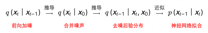
先验概率:根据以往经验和分析得到的概率,它往往作为“由因求果”问题中的“因”出现,如 q ( x t ∣ x t − 1 ) q(x_t|x_{t-1}) q(xt∣xt−1)
后验概率:指在得到“结果”的信息后重新修正的概率,是“执果寻因”问题中的“因", 如 p ( x t − 1 ∣ x t ) p(x_{t-1}|x_t) p(xt−1∣xt)
2、条件概率:设 A A A、 B B B为任意两个事件,若 P ( A ) > 0 P(A)>0 P(A)>0,称在已知事件 A A A发生的条件下,事件 B B B发生的概率为条件概率,记为 P ( B ∣ A ) P(B|A) P(B∣A)
P ( B ∣ A ) = P ( A , B ) P ( A ) P(B|A)=\frac{P(A,B)} {P(A)} P(B∣A)=P(A)P(A,B)
3、乘法公式:
P ( A , B ) = P ( B ∣ A ) P ( A ) P(A,B)=P(B|A)P(A) P(A,B)=P(B∣A)P(A)
4、乘法公式一般形式:
P ( A , B , C ) = P ( C ∣ B , A ) P ( B , A ) = P ( C ∣ B , A ) P ( B ∣ A ) P ( A ) P(A,B,C)=P(C|B,A)P(B,A)=P(C|B,A)P(B|A)P(A)\\ P(A,B,C)=P(C∣B,A)P(B,A)=P(C∣B,A)P(B∣A)P(A)
5、贝叶斯公式:
P ( A ∣ B ) = P ( B ∣ A ) P ( A ) P ( B ) P(A|B)=\frac{P(B|A)P(A)}{P(B)} P(A∣B)=P(B)P(B∣A)P(A)
6、多元贝叶斯公式:
P ( A ∣ B , C ) = P ( A , B , C ) P ( B , C ) = P ( B ∣ A , C ) P ( A , C ) P ( B , C ) = P ( B ∣ A , C ) P ( A ∣ C ) P ( C ) P ( B ∣ C ) P ( C ) = P ( B ∣ A , C ) P ( A ∣ C ) ) P ( B ∣ C ) P(A|B,C)=\frac{P(A,B,C)}{P(B,C)}=\frac{P(B|A,C)P(A,C)}{P(B,C)}=\frac{P(B|A,C)P(A|C)P(C)}{P(B|C)P(C)}=\frac{P(B|A,C)P(A|C))}{P(B|C)} P(A∣B,C)=P(B,C)P(A,B,C)=P(B,C)P(B∣A,C)P(A,C)=P(B∣C)P(C)P(B∣A,C)P(A∣C)P(C)=P(B∣C)P(B∣A,C)P(A∣C))
7、正态分布的叠加性:当有两个独立的正态分布变量 N 1 N_{1} N1和 N 2 N_{2} N2,它们的均值和方差分别为 μ 1 \mu_{1} μ1, μ 2 \mu_{2} μ2和 σ 1 2 \sigma_{1}^2 σ12, σ 2 2 \sigma_{2}^2 σ22它们的和为 N = a N 1 + b N 2 N=a N_{1}+b N_{2} N=aN1+bN2的均值和方差可以表示如下:
E ( N ) = E ( a N 1 + b N 2 ) = a μ 1 + b μ 2 V a r ( N ) = V a r ( a N 1 + b N 2 ) = a 2 σ 1 2 + b 2 σ 2 2 E(N)=E(aN_{1}+bN_{2})=a\mu_{1}+b\mu_{2}\\ Var(N)=Var(aN_{1}+bN_{2})=a^2\sigma_{1}^2+b^2\sigma_{2}^2 E(N)=E(aN1+bN2)=aμ1+bμ2Var(N)=Var(aN1+bN2)=a2σ12+b2σ22
相减时:
E ( N ) = E ( a N 1 − b N 2 ) = a μ 1 − b μ 2 V a r ( N ) = V a r ( a N 1 − b N 2 ) = a 2 σ 1 2 + b 2 σ 2 2 E(N)=E(aN_{1}-bN_{2})=a\mu_{1}-b\mu_{2}\\ Var(N)=Var(aN_{1}-bN_{2})=a^2\sigma_{1}^2+b^2\sigma_{2}^2 E(N)=E(aN1−bN2)=aμ1−bμ2Var(N)=Var(aN1−bN2)=a2σ12+b2σ22
8、重参数化:从 N ( μ , σ 2 ) N(\mu,\sigma^2) N(μ,σ2) 采样等价于从 N ( 0 , 1 ) N(0,1) N(0,1)采样一个 ϵ \epsilon ϵ, ϵ ⋅ σ + μ \epsilon\cdot\sigma+\mu ϵ⋅σ+μ
9、高斯分布的概率密度函数
f ( x ) = 1 2 π σ e − ( x − μ ) 2 2 σ 2 f(x)=\frac{1}{\sqrt{2\pi}\sigma}e^{-\frac{(x-\mu)^2}{2\sigma^2}} f(x)=2πσ1e−2σ2(x−μ)2
10、高斯分布的KL散度公式
K L ( p ∣ q ) = l o g σ 2 σ 1 + σ 2 + ( μ 1 − μ 2 ) 2 2 σ 2 2 − 1 2 KL(p|q)=log\frac{\sigma_2}{\sigma_1}+\frac{\sigma^2+(\mu_1-\mu_2)^2}{2\sigma_2^2}-\frac{1}{2} KL(p∣q)=logσ1σ2+2σ22σ2+(μ1−μ2)2−21
11、二次函数配方
a x 2 + b x = a ( x + b 2 a ) 2 + c ax^2+bx=a(x+\frac{b}{2a})^2+c ax2+bx=a(x+2ab)2+c
12、随机变量的期望公式
设 X X X是随机变量, Y = g ( X ) Y=g(X) Y=g(X),则:
E ( Y ) = E [ g ( X ) ] = { ∑ k = 1 ∞ g ( x k ) p k ∫ − ∞ ∞ g ( x ) p ( x ) d x E(Y)=E[g(X)]= \begin{cases} \displaystyle\sum_{k=1}^\infty g(x_k)p_k\\ \displaystyle\int_{-\infty}^{\infty}g(x)p(x)dx \end{cases} E(Y)=E[g(X)]=⎩ ⎨ ⎧k=1∑∞g(xk)pk∫−∞∞g(x)p(x)dx
13、KL散度公式
K L ( p ( x ) ∣ q ( x ) ) = E x ∼ p ( x ) [ p ( x ) q ( x ) ] = ∫ p ( x ) p ( x ) q ( x ) d x KL(p(x)|q(x))=E_{x \sim p(x)}[\frac{p(x)}{q(x)}]=\int p(x) \frac{p(x)}{q(x)}dx KL(p(x)∣q(x))=Ex∼p(x)[q(x)p(x)]=∫p(x)q(x)p(x)dx
介绍DDPM
2020年Berkeley提出DDPM(Denoising Diffusion Probabilistic Models),简称扩散模型,是AIGC的核心算法,在生成图像的真实性和多样性方面均超越了GAN,而且训练过程稳定。缺点是计算成本较高,实时推理比较困难,但也有相关技术在时间和空间维度上降低计算量。
扩散模型包括两个过程:前向扩散过程(前向加噪过程)和反向去噪过程。

前向过程和反向过程都是马尔可夫链,全过程大约需要1000步,其中反向过程用来生成数据,它的推导过程可以描述成:
前向扩散的过程
前向扩散过程是对原始数据逐渐增加高斯噪声,直至变成标准高斯分布的过程。

从原始数据集采样 x 0 ∼ q ( x 0 ) x_0\sim q(x_0) x0∼q(x0),按照预定义的noise schedule策略添加随机噪声,得到一系列噪声图像 x 1 , x 2 , … , x T x_1,x_2,\dots,x_T x1,x2,…,xT,用概率表示为:
q ( x 1 : T ∣ x 0 ) = ∏ t = 1 T q ( x t ∣ x t − 1 ) q ( x t ∣ x t − 1 ) = N ( x t ; α t x t − 1 , β t I ) \begin{aligned} q(x_{1:T}|x_{0})&=\prod_{t=1}^{T}q(x_t|x_{t-1}) \\q(x_{t}|x_{t-1})&=\mathcal{N}(x_t;\sqrt{\alpha_t}x_{t-1},\beta_{t}I)\\ \end{aligned} q(x1:T∣x0)q(xt∣xt−1)=t=1∏Tq(xt∣xt−1)=N(xt;αtxt−1,βtI)
进行重参数化(前置知识数学知识8),得到
x t = α t x t − 1 + β t ϵ t ϵ t ∼ N ( 0 , I ) α t = 1 − β t \begin{aligned} x_{t}&=\sqrt{\alpha_{t}}x_{t-1}+\sqrt{\beta_{t}}\epsilon_{t} \space \space \space \space \epsilon_{t}\sim \mathcal{N}(0,I) \\ \alpha_{t}&=1-\beta_{t} \end{aligned} xtαt=αtxt−1+βtϵt ϵt∼N(0,I)=1−βt
利用上述公式进行迭代推导
x t = α t x t − 1 + β t ϵ t = α t ( α t − 1 x t − 2 + β t − 1 ϵ t − 1 ) + β t ϵ t = ( α t … α 1 ) x 0 + ( α t … α 2 ) β 1 ϵ 1 + ( α t … α 3 ) β 2 ϵ 2 + ⋯ + α t β t − 1 ϵ t − 1 + β t ϵ t \begin{aligned} x_{t}&=\sqrt{\alpha_{t}} x_{t-1}+\sqrt{\beta_{t}}\epsilon_{t}\\ &=\sqrt{\alpha_{t}}(\sqrt{\alpha_{t-1}}x_{t-2}+\sqrt{\beta_{t-1}}\epsilon_{t-1})+\sqrt{\beta_{t}}\epsilon_{t}\\ &=\sqrt{(\alpha_{t}\dots\alpha_{1})}x_{0}+\sqrt{(\alpha_{t}\dots\alpha_{2})\beta_{1}}\epsilon_{1}+\sqrt{(\alpha_{t}\dots\alpha_{3})\beta_{2}}\epsilon_{2}+\dots+\sqrt{\alpha_{t}\beta_{t-1}}\epsilon_{t-1}+\sqrt{\beta_{t}}\epsilon_{t} \end{aligned} xt=αtxt−1+βtϵt=αt(αt−1xt−2+βt−1ϵt−1)+βtϵt=(αt…α1)x0+(αt…α2)β1ϵ1+(αt…α3)β2ϵ2+⋯+αtβt−1ϵt−1+βtϵt
设: α t ˉ = α 1 α 2 … α t \bar{\alpha_{t}}=\alpha_{1}\alpha_{2}\dots\alpha_{t} αtˉ=α1α2…αt
根据正态分布的叠加性得到
x t = α t ˉ x 0 + 1 − α t ˉ ϵ ϵ ∼ N ( 0 , I ) q ( x t ∣ x 0 ) = N ( x t ; α t ˉ x 0 , 1 − α t ˉ I ) x_{t}=\sqrt{\bar{\alpha_{t}}}x_{0}+\sqrt{1-\bar{\alpha_{t}}}\epsilon \space \space\space \epsilon\sim \mathcal{N}(0,I)\\ \textcolor{REd}{q(x_{t}|x_{0})=\mathcal{N}(x_{t};\sqrt{\bar{\alpha_{t}}}x_{0},\sqrt{1-\bar{\alpha_{t}}}I)} xt=αtˉx0+1−αtˉϵ ϵ∼N(0,I)q(xt∣x0)=N(xt;αtˉx0,1−αtˉI)
这个公式表示任意步骤 t t t的噪声图像 x t x_t xt ,都可以通过 x 0 x_0 x0直接加噪得到,后面需要用到。
注:上述前向过程在代码实现时是一步到位的!!!!!
反向去噪过程,神经网络拟合过程
反向去噪过程就是数据生成过程,它首先是从标准高斯分布中采样得到一个噪声样本,再一步步地迭代去噪,最后得到数据分布中的一个样本。

如果知道反向过程的每一步真实的条件分布 q ( x t − 1 ∣ x t ) q(x_{t-1}|x_t) q(xt−1∣xt),那么从一个随机噪声开始,逐步采样就能生成一个真实的样本。但是真实的条件分布利用贝叶斯公式
q ( x t − 1 ∣ x t ) = q ( x t ∣ x t − 1 ) q ( x t − 1 ) q ( x t ) q(x_{t-1}|x_{t}) =\frac{q(x_{t}|x_{t-1})q(x_{t-1})}{q(x_{t})} q(xt−1∣xt)=q(xt)q(xt∣xt−1)q(xt−1)
无法直接求解,原因是其中 q ( x t − 1 ) q(x_{t-1}) q(xt−1) , q ( x t ) q(x_{t}) q(xt) 未知,因此无法从 x t x_{t} xt 推导到 x t − 1 {x_{t-1}} xt−1,所以必须通过神经网络** p θ ( x t − 1 ∣ x t ) p_\theta(x_{t-1}|x_t) pθ(xt−1∣xt)来近似。为了简化起见,将反向过程也定义为一个马尔卡夫链,且服从高斯分布**,建模如下:
p θ ( x 0 : T ) = p ( x T ) ∏ t = 1 T p θ ( x t − 1 ∣ x t ) p θ ( x t − 1 ∣ x t ) = N ( x t − 1 ; μ θ ( x t , t ) , ∑ θ ( x t , t ) ) p_\theta(x_{0:T})=p(x_T)\prod_{t=1}^Tp_\theta(x_{t-1}|x_t)\\ p_\theta(x_{t-1}|x_t)=N(x_{t-1};\mu_\theta(x_t,t),\sum_\theta(x_t,t)) pθ(x0:T)=p(xT)t=1∏Tpθ(xt−1∣xt)pθ(xt−1∣xt)=N(xt−1;μθ(xt,t),θ∑(xt,t))
--------------------下面这段讲解与上面有些跳脱,是为损失函数做铺垫------------------------------
虽然真实条件分布 q ( x t − 1 ∣ x t ) q(x_{t-1}|x_t) q(xt−1∣xt)无法直接求解,但是加上已知条件 x 0 x_0 x0的后验分布$q(x_{t-1}|x_{t},x_{0}) $却可以通过贝叶斯公式求解,再结合前向马尔科夫性质可得:
q ( x t − 1 ∣ x t , x 0 ) = q ( x t ∣ x t − 1 , x 0 ) q ( x t − 1 ∣ x 0 ) q ( x t ∣ x 0 ) = q ( x t ∣ x t − 1 ) q ( x t − 1 ∣ x 0 ) q ( x t ∣ x 0 ) q(x_{t-1}|x_{t},x_{0}) =\frac{q(x_{t}|x_{t-1},x_{0})q(x_{t-1}|x_{0})}{q(x_{t}|x_{0})}=\frac{q(x_{t}|x_{t-1})q(x_{t-1}|x_{0})}{q(x_{t}|x_{0})} q(xt−1∣xt,x0)=q(xt∣x0)q(xt∣xt−1,x0)q(xt−1∣x0)=q(xt∣x0)q(xt∣xt−1)q(xt−1∣x0)
因此可以得到:
q ( x t − 1 ∣ x 0 ) = α ˉ t − 1 x 0 + 1 − α ˉ t − 1 ϵ ∼ N ( α ˉ t − 1 x 0 , ( 1 − α ˉ t − 1 ) I ) q ( x t ∣ x 0 ) = α ˉ t x 0 + 1 − α ˉ t ϵ ∼ N ( α ˉ t x 0 , ( 1 − α ˉ t ) I ) q ( x t ∣ x t − 1 ) = α t x t − 1 + β t ϵ ∼ N ( α t x t − 1 , β t I ) \begin{aligned} q(x_{t-1}|x_{0})&=\sqrt{\bar{\alpha}_{t-1}}x_{0}+\sqrt{1-\bar{\alpha}_{t-1}}\epsilon\sim \mathcal{N}(\sqrt{\bar{\alpha}_{t-1}}x_{0},(1-\bar{\alpha}_{t-1})I)\\ q(x_{t}|x_{0})&=\sqrt{\bar{\alpha}_{t}}x_{0}+\sqrt{1-\bar{\alpha}_{t}}\epsilon\sim \mathcal{N}(\sqrt{\bar{\alpha}_{t}}x_{0},(1-\bar{\alpha}_{t})I)\\ q(x_{t}|x_{t-1})&=\sqrt{\alpha}_{t}x_{t-1}+\beta_{t}\epsilon\sim \mathcal{N}(\sqrt{\alpha}_{t}x_{t-1},\beta_{t}I) \end{aligned} q(xt−1∣x0)q(xt∣x0)q(xt∣xt−1)=αˉt−1x0+1−αˉt−1ϵ∼N(αˉt−1x0,(1−αˉt−1)I)=αˉtx0+1−αˉtϵ∼N(αˉtx0,(1−αˉt)I)=αtxt−1+βtϵ∼N(αtxt−1,βtI)
所以
q ( x t − 1 ∣ x t , x 0 ) ∝ e x p ( − 1 2 ( ( x t − α t x t − 1 ) 2 β t ) + ( x t − 1 − α ˉ t − 1 x 0 ) 2 1 − α ˉ t − 1 − ( x t − α ˉ t x 0 ) 2 1 − α ˉ t ) = e x p ( − 1 2 ( α t β t + 1 1 − α ˉ t − 1 ) x t − 1 2 − ( 2 α t β t x t + 2 α t ˉ 1 − α t ˉ x 0 ) x t − 1 + C ( x t , x 0 ) ) \begin{aligned} q(x_{t-1}|x_{t},x_{0}) &\propto exp(-\frac{1}{2}(\frac{(x_{t}-\sqrt{\alpha_{t}}x_{t-1})^2}{\beta_{t}})+\frac{(x_{t-1}-\sqrt{\bar{\alpha}}_{t-1}x_{0})^2}{1-\bar{\alpha}_{t-1}}-\frac{(x_{t}-\sqrt{\bar{\alpha}_{t}}x_{0})^2}{1-\bar{\alpha}_{t}})\\ &=exp(-\frac{1}{2}(\frac{\alpha_{t}}{\beta_{t}}+\frac{1}{1-\bar{\alpha}_{t-1}})x_{t-1}^2-(\frac{2\sqrt{\alpha_{t}}}{\beta_{t}}x_{t}+\frac{2\sqrt{\bar{\alpha_{t}}}}{1-\bar{\alpha_{t}}}x_{0})x_{t-1}+C(x_{t},x_{0})) \end{aligned} q(xt−1∣xt,x0)∝exp(−21(βt(xt−αtxt−1)2)+1−αˉt−1(xt−1−αˉt−1x0)2−1−αˉt(xt−αˉtx0)2)=exp(−21(βtαt+1−αˉt−11)xt−12−(βt2αtxt+1−αtˉ2αtˉx0)xt−1+C(xt,x0))
通过配方就可以得到
β ~ t = 1 / ( α t β t + 1 1 − α ˉ t − 1 ) = 1 − α ˉ t − 1 1 − α ˉ t β t μ ~ t = ( α t β t x t + α ˉ t 1 − α t ˉ x 0 ) / ( α t β t + 1 1 − α ˉ t − 1 ) = α t ( 1 − α ˉ t − 1 ) 1 − α t ˉ x t + α ˉ t − 1 β t 1 − α ˉ t x 0 \widetilde{\beta}_t=1/(\frac{\alpha_{t}}{\beta_{t}}+\frac{1}{1-\bar{\alpha}_{t-1}})=\frac{1-\bar{\alpha}_{t-1}}{1-\bar{\alpha}_{t}}\beta_{t}\\ \widetilde{\mu}_t=(\frac{\sqrt\alpha_{t}}{\beta_{t}}x_{t}+\frac{\sqrt{\bar{\alpha}_{t}}}{1-\bar{\alpha_{t}}}x_{0})/(\frac{\alpha_{t}}{\beta_{t}}+\frac{1}{1-\bar{\alpha}_{t-1}})=\frac{\sqrt{\alpha_{t}}(1-\bar{\alpha}_{t-1})}{1-\bar{\alpha_{t}}}x_{t}+\frac{\sqrt{\bar{\alpha}_{t-1}}\beta_{t}}{1-\bar{\alpha}_{t}}x_{0} β t=1/(βtαt+1−αˉt−11)=1−αˉt1−αˉt−1βtμ t=(βtαtxt+1−αtˉαˉtx0)/(βtαt+1−αˉt−11)=1−αtˉαt(1−αˉt−1)xt+1−αˉtαˉt−1βtx0
又因为
x 0 = 1 α ˉ t ( x t − β t 1 − α ˉ t ϵ ) x_0= \frac{1}{\sqrt{\bar\alpha_t}}(x_t- \frac{\beta_t}{\sqrt{1-\bar \alpha_t} }\epsilon)\\ x0=αˉt1(xt−1−αˉtβtϵ)
可以得
μ ~ t = 1 α t ( x t − β t ( 1 − α t ) ϵ ) \widetilde{\mu}_t=\frac{1}{\sqrt{\alpha_t} }(x_t-\frac{\beta_t}{\sqrt{(1-\alpha_t)}}\epsilon) μ t=αt1(xt−(1−αt)βtϵ)
----------------------------------------------------------------------------------------------
采样过程(模型训练完后的预测过程)
μ θ ( x t , t ) = 1 α t ( x t − β t ( 1 − α t ) ϵ θ ( x t , t ) ) x t − 1 ∼ p θ ( x t − 1 ∣ x t ) x t − 1 = 1 α t ( x t − β t ( 1 − α t ) ϵ θ ( x t , t ) ) + β ~ t z z ∼ N ( 0 , I ) \mu_\theta(x_t,t)=\frac{1}{\sqrt{\alpha_t} }(x_t-\frac{\beta_t}{\sqrt{(1-\alpha_t)}}\epsilon_\theta(x_t,t))\\ x_{t-1}\sim p_\theta(x_{t-1}|x_t)\\ x_{t-1}=\frac{1}{\sqrt{\alpha_t} }(x_t-\frac{\beta_t}{\sqrt{(1-\alpha_t)}}\epsilon_\theta(x_t,t))+\sqrt{\widetilde{\beta}_t}z \space \space\space\space z\sim N(0,I) μθ(xt,t)=αt1(xt−(1−αt)βtϵθ(xt,t))xt−1∼pθ(xt−1∣xt)xt−1=αt1(xt−(1−αt)βtϵθ(xt,t))+β tz z∼N(0,I)
这里用z是为了和之前的 ϵ \epsilon ϵ区别开
损失函数
https://blog.csdn.net/weixin_45453121/article/details/131223653
Code
import torch
import torchvision
import matplotlib.pyplot as plt
import torch.nn.functional as F
from torchvision import transforms
from torch.utils.data import DataLoader
import numpy as np
from torch.optim import Adam
from torch import nn
import math
from torchvision.utils import save_imagedef show_images(data, num_samples=20, cols=4):""" Plots some samples from the dataset """plt.figure(figsize=(15,15))for i, img in enumerate(data):if i == num_samples:breakplt.subplot(int(num_samples/cols) + 1, cols, i + 1)plt.imshow(img[0])def linear_beta_schedule(timesteps, start=0.0001, end=0.02):return torch.linspace(start, end, timesteps)def get_index_from_list(vals, t, x_shape):"""Returns a specific index t of a passed list of values valswhile considering the batch dimension."""batch_size = t.shape[0]out = vals.gather(-1, t.cpu())#print("out:",out)#print("out.shape:",out.shape)return out.reshape(batch_size, *((1,) * (len(x_shape) - 1))).to(t.device)def forward_diffusion_sample(x_0, t, device="cpu"):"""Takes an image and a timestep as input andreturns the noisy version of it"""noise = torch.randn_like(x_0)sqrt_alphas_cumprod_t = get_index_from_list(sqrt_alphas_cumprod, t, x_0.shape)sqrt_one_minus_alphas_cumprod_t = get_index_from_list(sqrt_one_minus_alphas_cumprod, t, x_0.shape)# mean + variancereturn sqrt_alphas_cumprod_t.to(device) * x_0.to(device) \+ sqrt_one_minus_alphas_cumprod_t.to(device) * noise.to(device), noise.to(device)def load_transformed_dataset(IMG_SIZE):data_transforms = [transforms.Resize((IMG_SIZE, IMG_SIZE)),transforms.ToTensor(), # Scales data into [0,1]transforms.Lambda(lambda t: (t * 2) - 1) # Scale between [-1, 1]]data_transform = transforms.Compose(data_transforms)train = torchvision.datasets.MNIST(root="./Data",transform=data_transform,train=True)test = torchvision.datasets.MNIST(root="./Data", transform=data_transform, train=False)return torch.utils.data.ConcatDataset([train, test])def show_tensor_image(image):reverse_transforms = transforms.Compose([transforms.Lambda(lambda t: (t + 1) / 2),transforms.Lambda(lambda t: t.permute(1, 2, 0)), # CHW to HWCtransforms.Lambda(lambda t: t * 255.),transforms.Lambda(lambda t: t.numpy().astype(np.uint8)),transforms.ToPILImage(),])#Take first image of batchif len(image.shape) == 4:image = image[0, :, :, :]plt.imshow(reverse_transforms(image))class Block(nn.Module):def __init__(self, in_ch, out_ch, time_emb_dim, up=False):super().__init__()self.time_mlp =  nn.Linear(time_emb_dim, out_ch)if up:self.conv1 = nn.Conv2d(2*in_ch, out_ch, 3, padding=1)self.transform = nn.ConvTranspose2d(out_ch, out_ch, 4, 2, 1)else:self.conv1 = nn.Conv2d(in_ch, out_ch, 3, padding=1)self.transform = nn.Conv2d(out_ch, out_ch, 4, 2, 1)self.conv2 = nn.Conv2d(out_ch, out_ch, 3, padding=1)self.bnorm1 = nn.BatchNorm2d(out_ch)self.bnorm2 = nn.BatchNorm2d(out_ch)self.relu  = nn.ReLU()def forward(self, x, t):#print("ttt:",t.shape)# First Convh = self.bnorm1(self.relu(self.conv1(x)))# Time embeddingtime_emb = self.relu(self.time_mlp(t))# Extend last 2 dimensionstime_emb = time_emb[(..., ) + (None, ) * 2]# Add time channelh = h + time_emb# Second Convh = self.bnorm2(self.relu(self.conv2(h)))# Down or Upsamplereturn self.transform(h)class SinusoidalPositionEmbeddings(nn.Module):def __init__(self, dim):super().__init__()self.dim = dimdef forward(self, time):device = time.devicehalf_dim = self.dim // 2embeddings = math.log(10000) / (half_dim - 1)embeddings = torch.exp(torch.arange(half_dim, device=device) * -embeddings)embeddings = time[:, None] * embeddings[None, :]embeddings = torch.cat((embeddings.sin(), embeddings.cos()), dim=-1)# TODO: Double check the ordering herereturn embeddingsclass SimpleUnet(nn.Module):"""A simplified variant of the Unet architecture."""def __init__(self):super().__init__()image_channels =1   #灰度图为1,彩色图为3down_channels = (64, 128, 256, 512, 1024)up_channels = (1024, 512, 256, 128, 64)out_dim = 1   #灰度图为1 ,彩色图为3time_emb_dim = 32# Time embeddingself.time_mlp = nn.Sequential(SinusoidalPositionEmbeddings(time_emb_dim),nn.Linear(time_emb_dim, time_emb_dim),nn.ReLU())# Initial projectionself.conv0 = nn.Conv2d(image_channels, down_channels[0], 3, padding=1)# Downsampleself.downs = nn.ModuleList([Block(down_channels[i], down_channels[i+1], \time_emb_dim) \for i in range(len(down_channels)-1)])# Upsampleself.ups = nn.ModuleList([Block(up_channels[i], up_channels[i+1], \time_emb_dim, up=True) \for i in range(len(up_channels)-1)])# Edit: Corrected a bug found by Jakub C (see YouTube comment)self.output = nn.Conv2d(up_channels[-1], out_dim, 1)def forward(self, x, timestep):# Embedd timet = self.time_mlp(timestep)# Initial convx = self.conv0(x)# Unetresidual_inputs = []for down in self.downs:x = down(x, t)residual_inputs.append(x)for up in self.ups:residual_x = residual_inputs.pop()# Add residual x as additional channelsx = torch.cat((x, residual_x), dim=1)x = up(x, t)return self.output(x)def get_loss(model, x_0, t):x_noisy, noise = forward_diffusion_sample(x_0, t, device)noise_pred = model(x_noisy, t)return F.l1_loss(noise, noise_pred)@torch.no_grad()
def sample_timestep(x, t):"""Calls the model to predict the noise in the image and returnsthe denoised image.Applies noise to this image, if we are not in the last step yet."""betas_t = get_index_from_list(betas, t, x.shape)sqrt_one_minus_alphas_cumprod_t = get_index_from_list(sqrt_one_minus_alphas_cumprod, t, x.shape)sqrt_recip_alphas_t = get_index_from_list(sqrt_recip_alphas, t, x.shape)# Call model (current image - noise prediction)model_mean = sqrt_recip_alphas_t * (x - betas_t * model(x, t) / sqrt_one_minus_alphas_cumprod_t)posterior_variance_t = get_index_from_list(posterior_variance, t, x.shape)if t == 0:# As pointed out by Luis Pereira (see YouTube comment)# The t's are offset from the t's in the paperreturn model_meanelse:noise = torch.randn_like(x)return model_mean + torch.sqrt(posterior_variance_t) * noise@torch.no_grad()
def sample_plot_image(IMG_SIZE):# Sample noiseimg_size = IMG_SIZEimg = torch.randn((1, 1, img_size, img_size), device=device)   #生成第T步的图片plt.figure(figsize=(15,15))plt.axis('off')num_images = 10stepsize = int(T/num_images)for i in range(0,T)[::-1]:t = torch.full((1,), i, device=device, dtype=torch.long)#print("t:",t)img = sample_timestep(img, t)# Edit: This is to maintain the natural range of the distributionimg = torch.clamp(img, -1.0, 1.0)if i % stepsize == 0:plt.subplot(1, num_images, int(i/stepsize)+1)plt.title(str(i))show_tensor_image(img.detach().cpu())plt.show()if __name__ =="__main__":# Define beta scheduleT = 300betas = linear_beta_schedule(timesteps=T)# Pre-calculate different terms for closed formalphas = 1. - betasalphas_cumprod = torch.cumprod(alphas, axis=0)# print(alphas_cumprod.shape)alphas_cumprod_prev = F.pad(alphas_cumprod[:-1], (1, 0), value=1.0)# print(alphas_cumprod_prev)# print(alphas_cumprod_prev.shape)sqrt_recip_alphas = torch.sqrt(1.0 / alphas)sqrt_alphas_cumprod = torch.sqrt(alphas_cumprod)sqrt_one_minus_alphas_cumprod = torch.sqrt(1. - alphas_cumprod)posterior_variance = betas * (1. - alphas_cumprod_prev) / (1. - alphas_cumprod)# print(posterior_variance.shape)IMG_SIZE = 32BATCH_SIZE = 16data = load_transformed_dataset(IMG_SIZE)dataloader = DataLoader(data, batch_size=BATCH_SIZE, shuffle=True, drop_last=True)model = SimpleUnet()print("Num params: ", sum(p.numel() for p in model.parameters()))device = "cuda" if torch.cuda.is_available() else "cpu"model.to(device)optimizer = Adam(model.parameters(), lr=0.001)epochs = 1 # Try more!for epoch in range(epochs):for step, batch in enumerate(dataloader):  #由于batch 是包含标签的所以取batch[0]#print(batch[0].shape)optimizer.zero_grad()t = torch.randint(0, T, (BATCH_SIZE,), device=device).long()loss = get_loss(model, batch[0], t)loss.backward()optimizer.step()if epoch % 1 == 0 and step %5== 0:print(f"Epoch {epoch} | step {step:03d} Loss: {loss.item()} ")sample_plot_image(IMG_SIZE)
参考文献
https://zhuanlan.zhihu.com/p/630354327](https://zhuanlan.zhihu.com/p/630354327)
https://blog.csdn.net/weixin_45453121/article/details/131223653
https://www.cnblogs.com/risejl/p/17448442.html
https://zhuanlan.zhihu.com/p/569994589?utm_id=0
相关文章:
深度学习——(生成模型)DDPM
前置数学知识 1、先验概率和后验概率 先验概率:根据以往经验和分析得到的概率,它往往作为“由因求果”问题中的“因”出现,如 q ( x t ∣ x t − 1 ) q(x_t|x_{t-1}) q(xt∣xt−1) 后验概率:指在得到“结果”的信息后重新修正的概率,是…...

uniapp如何使用api相关提示框
uni.showToast:用于显示一条带有图标的提示框。title:提示的内容。icon:图标,可选值包括 success、loading、none。duration:提示框持续时间(单位:毫秒),默认为1500。 un…...
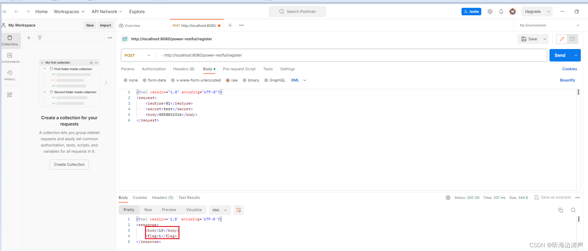
在Java代码中指定用JAXB的XmlElement注解的元素的顺序
例如,下面的类RegisterResponse 使用了XmlRootElement注解,同时也使用XmlType注解,并用XmlType注解的propOrder属性,指定了两个用XmlElement注解的元素出现的顺序,先出现flag,后出现enterpriseId࿰…...
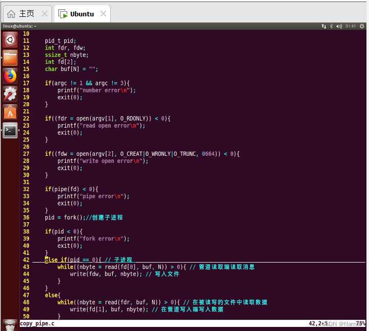
Linux 基本语句_11_无名管道文件复制
父子进程: 父子进程的变量之间存在着读时共享,写时复制原则 无名管道: 无名管道仅能用于有亲缘关系的进程之间通信如父子进程 代码: #include <stdio.h> #include <unistd.h> #include <sys/types.h> #inc…...
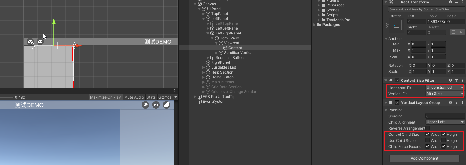
侧面多级菜单(一个大类、一个小类、小类下多个物体)
效果: 说明: 左右侧面板使用Animator组件控制滑入滑出。左侧面板中,左的左里面是大类,左的右有绿色的小类,绿色的小类下有多个真正的UI图片按钮。 要点: 结合了一点EasyGridBuilderPro插件的UI元素&…...
、( 什么是qps,tps,并发量,pv,uv)、(什么是接口幂等性问题,如何解决?))
2-(脏读,不可重复读,幻读 ,mysql5.7以后默认隔离级别)、( 什么是qps,tps,并发量,pv,uv)、(什么是接口幂等性问题,如何解决?)
1 脏读,不可重复读,幻读 ,mysql5.7以后默认隔离级别是什么? 2 什么是qps,tps,并发量,pv,uv 3 什么是接口幂等性问题,如何解决? 1 脏读,不可重复读…...

wpf devexpress 创建布局
模板解决方案 例子是一个演示连接数据库连接程序。打开RegistrationForm.BaseProject项目和如下步骤 RegistrationForm.Lesson1 项目包含结果 审查Form设计 使用LayoutControl套件创建混合控件和布局 LayoutControl套件包含三个主控件: LayoutControl - 根布局…...

Chrome 浏览器经常卡死问题解决
Chrome 浏览器经常卡死问题解决 打开WX, 搜索“程序员奇点” chrome 任务管理器杀进程 mac 后台有很多 google chrome helper 线程并且内存占用较高 一直怀疑是插件的锅 其实并不是-0- 查看是哪个网页,哪个插件占用内存 chrome 更多工具 -> 任务管理器 切换到…...

listbox控件响应鼠标右键消息
众所周知,对话框中的listbox控件无法响应鼠标消息。 但是,使用SetWindowPtrLong API函数,然后在新的窗口处理程序中,可以响应WM_RBUTTONDOWN等鼠标消息。代码非常简单,暂不提供,自己测试即可。...
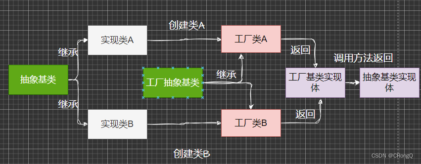
设计模式(二)-创建者模式(2)-工厂模式
一、为何需要工厂模式(Factory Pattern)? 由于简单工厂模式存在一个缺点,如果工厂类创建的对象过多,使得代码变得越来越臃肿。这样导致工厂类难以扩展新实例,以及难以维护代码逻辑。于是在简单工厂模式的基础上&…...

2023年高压电工证考试题库及高压电工试题解析
题库来源:安全生产模拟考试一点通公众号小程序 2023年高压电工证考试题库及高压电工试题解析是安全生产模拟考试一点通结合(安监局)特种作业人员操作证考试大纲和(质检局)特种设备作业人员上岗证考试大纲随机出的高压…...

公网访问全能知识库工具AFFINE,Notion的免费开源替代
文章目录 公网访问全能知识库工具AFFINE,Notion的免费开源替代品前言1. 使用Docker安装AFFINE2. 安装cpolar内网穿透工具3. 配置AFFINE公网访问地址4. 实现公网远程访问AFFINE 公网访问全能知识库工具AFFINE,Notion的免费开源替代品 前言 AFFiNE 是一个…...

数据存储模型
1、前言 写点什么东西呢 之前大学毕设搞了个高并发模型,里面使用到了select模型,里面用到了一个内存池,支持多客户端连接、登录、消息发送,现在工作经验三年多了,开发经验积累了不少,但是对喜爱的C的一些知…...

vue3+vant 实现树状多选组件
vue3vant 实现树状多选组件 需求描述效果图代码父组件引用selectTree组件 tree组件数据格式 需求描述 移动端需要复刻Pc端如上图的功能组件,但vant无组件可用,所以自己封装一个。 效果图 代码 父组件引用 import TreeSelect from "/selectTree.vu…...
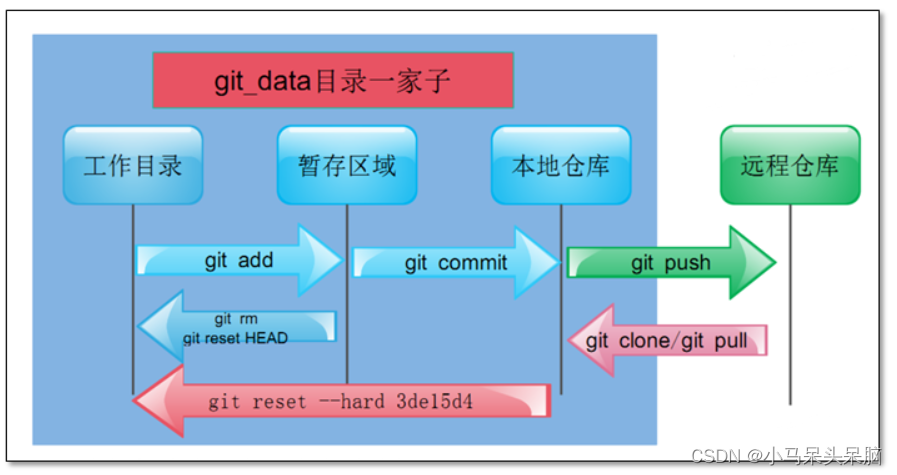
Git安装与常用命令
Git简介: Git是一个开源的分布式版本控制系统,用于敏捷高效地处理任何或大或小的项目。Git是Linus Torvalds为了帮助管理Linux内核开发而开发的一个开放源代码的版本控制软件。Git与常用的版本控制工具CVS、Subversion等不同,它采用了分布式…...
uni-app 使用vscode开发uni-app
安装插件 uni-create-view 用于快速创建页面 配置插件 创建页面 输入页面名称,空格,顶部导航的标题,回车 自动生成页面并在pages.json中注册了路由 pages\login\login.vue <template><div class"login">login</d…...
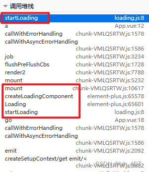
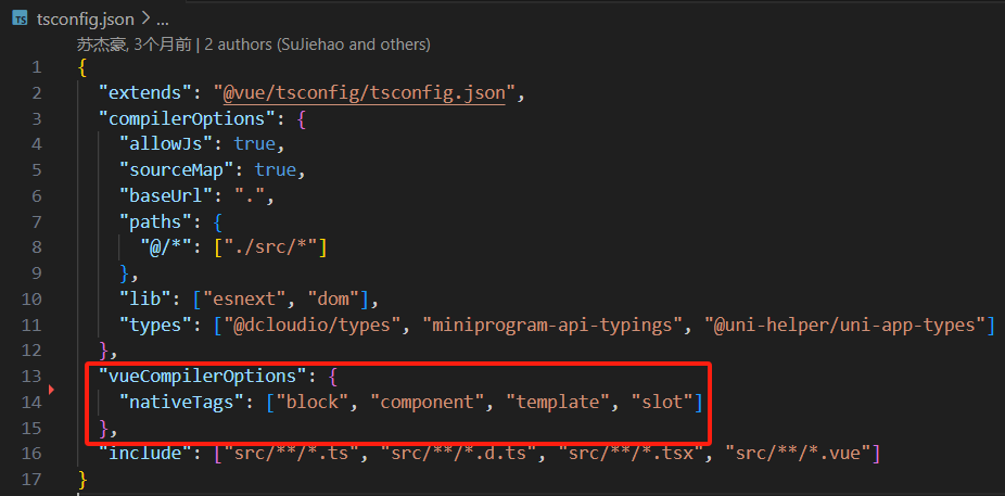
单线程的JS中Vue导致的“线程安全”问题
目录 现象分析原因 浏览器中Js是单线程的,当然不可能出现线程安全问题。只是遇到的问题的现象与多线程的情况十分相似,导致对不了解Vue实现的我怀疑起了人生… 现象 项目中用到了element-plus中的加载组件,简单封装了一下,用来保…...

vue2 - SuperMap3D加载基于Nginx服务生成的3DTileset模型切片服务地址
文章目录 🍍开发环境🍉1:nginx发布3Dtileset模型切片服务🍍1.1:准备3DTileset文件🍍1.2:安装nginx服务,配置相关文件1.2.1:下载nginx1.2.2:下载完解压文件如下1.2.3:将3Dtileset模型文件放置 nginx-1.24.0/html/gc 新建文件中如下:1.2.4:配置nginx服务🍉2:…...

新版本Spring Security 2.7 + 用法,直接旧正版粘贴
一、以前的用法: Configuration public class SecurityConfig extends WebSecurityConfigurerAdapter {Beanpublic PasswordEncoder passwordEncoder(){return new BCryptPasswordEncoder();}Overrideprotected void configure(HttpSecurity http) throws Exceptio…...
JVM——类加载器(JDK8及之前,双亲委派机制)
目录 1.类加载器的分类1.实现方式分类1.虚拟机底层实现2.JDK中默认提供或者自定义 2.类加载器的分类-启动类加载器3.类加载器的分类-Java中的默认类加载器4.类加载器的分类-扩展类加载器5.类加载器的分类-类加载器的继承 2.类加载器的双亲委派机制 类加载器(ClassLo…...
—东方仙盟)
酒店门锁V10SDK接口说明-幽冥大陆(一百23)—东方仙盟
相关文件系统环境C# :NET.20,NET3.5,NET4,NET4.5,NET 5.0C:VS2005,VS2012,VS2015操作系统:未来之窗VOSWEB:CHROME43核心代码完整代码using System; using System.Collections.Generic; using System.Text; using System.Collections.Specialized;using System.Windo…...
)
别再只测accuracy!DeepSeek集成测试必须监控的5个隐性指标(P99首token延迟、context bleed率、tool-call schema漂移)
更多请点击: https://intelliparadigm.com 第一章:DeepSeek集成测试的核心范式演进 DeepSeek大模型的工程化落地对集成测试提出了全新挑战:传统基于接口响应码与字段校验的测试范式已难以覆盖语义一致性、推理链鲁棒性、上下文敏感度等高阶质…...

GEO生成引擎优化:当AI成为信息分发的主角,品牌如何抢占对话窗口?
当用户不再"搜索-浏览",而是直接"AI提问-获取答案",传统SEO的逻辑正在被彻底改写。2026年,GEO(Generative Engine Optimization,生成式引擎优化)已经从概念走向规模化落地。本文从技术…...

艾尔登法环存档迁移终极指南:3分钟解决角色转移难题
艾尔登法环存档迁移终极指南:3分钟解决角色转移难题 【免费下载链接】EldenRingSaveCopier 项目地址: https://gitcode.com/gh_mirrors/el/EldenRingSaveCopier 还在为《艾尔登法环》存档版本不兼容而烦恼吗?EldenRingSaveCopier 是你的终极解决…...

百度深度学习研究院的“叛将“,带着一颗芯片改变了中国智能驾驶——地平线余凯,从ImageNet冠军到征程出货1000万
大家好,我是写代码的篮球球痴。这篇文章跟我自己有点关系——我开的是理想汽车。理想的智驾系统 AD Pro,搭载的就是地平线征程 5 芯片。2026 年 1 月理想 AD Pro 4.0 推送,基于单颗征程 6M 实现了城市 NOA——这是行业里第一个用单颗 128TOPS…...

危急时刻的六条基本安全提示
人机协作,AI模型:Deepseek 仅供参考 危急时刻的六条基本安全提示 以下内容仅为通用性安全建议,供在紧急情况下保持冷静、保护自身安全时参考。所有建议均基于常理和公共安全常识,不包含任何具体操作细节或可能被不当使用的信息…...

告别坐标点击!用Poco精准定位UI控件,让你的Airtest安卓自动化脚本更稳定
告别坐标点击!用Poco精准定位UI控件,让你的Airtest安卓自动化脚本更稳定每次UI微调就导致脚本大面积失效?分辨率变化让精心编写的自动化测试瞬间崩溃?作为从坐标点击转型到控件识别的实践者,我深刻理解这种挫败感。三年…...

原神私服新纪元:KCN-GenshinServer图形化服务端全功能解析
原神私服新纪元:KCN-GenshinServer图形化服务端全功能解析 【免费下载链接】KCN-GenshinServer 基于GC制作的原神一键GUI多功能服务端。 项目地址: https://gitcode.com/gh_mirrors/kc/KCN-GenshinServer 你是否曾想过拥有一个完全由自己掌控的提瓦特大陆&am…...

深度解析:JetBrains IDE试用期重置机制的技术实现
深度解析:JetBrains IDE试用期重置机制的技术实现 【免费下载链接】ide-eval-resetter 项目地址: https://gitcode.com/gh_mirrors/id/ide-eval-resetter 在软件开发工作流中,JetBrains IDE试用期管理是一个常见的技术挑战,尤其是在多…...

别让依赖毁了你的实验:记一次Vision Mamba复现中causal_conv1d与mamba-ssm的版本“打架”事件
Vision Mamba复现实战:破解依赖冲突的工程化解决方案在深度学习项目的复现过程中,依赖管理往往是最容易被忽视却又最常导致问题的环节。最近在复现Vision Mamba模型时,我遭遇了一场典型的Python依赖"战争"——causal_conv1d与mamba…...