R语言:利用biomod2进行生态位建模
在这里主要是分享一个不错的代码,喜欢的可以慢慢研究。我看了一遍,觉得里面有很多有意思的东西,供大家学习和参考。

利用PCA轴总结的70个环境变量,利用biomod2进行生态位建模:
#----------------------------------------------------------#
# NICHE MODELLING WITH BIOMOD2 USING #######
# 70 ENVIRONMENTAL VARIABLES (10-km RESOLUTION) #######
# SUMMARIZED IN PCA AXES #######
#-------------------------------------------------------## Contact: Pedro V. Eisenlohr (pedro.eisenlohr@unemat.br)#------------------------------------------------- Acknowledgments ------------------------------------------------------------####
### Dr. Guarino Colli's team of Universidade de BrasÃlia. #########################################################################
### Dr. Diogo Souza Bezerra Rocha (Instituto de Pesquisas Jardim Botânico/RJ). ####################################################
### Drª Marinez Ferreira de Siqueira (Instituto de Pesquisas Jardim Botânico/RJ). #################################################
### My students of Ecology Lab, mainly J.C. Pires-de-Oliveira. ####################################################################
#----------------------------------------- ---------------------------------------------------------------------------------------##------------------------------------------------------------------------------------------------------------------------------------------------------------------------------------#
### Environmental data source (70 variables):### Temperature and precipitation (19 variables): CHELSA (http://chelsa-climate.org/).#Bio1 = Annual Mean Temperature#Bio2 = Mean Diurnal Range#Bio3 = Isothermality#Bio4 = Temperature Seasonality#Bio5 = Max Temperature of Warmest Month#Bio6 = Min Temperature of Coldest Month#Bio7 = Temperature Annual Range#Bio8 = Mean Temperature of Wettest Quarter#Bio9 = Mean Temperature of Driest Quarter#Bio10 = Mean Temperature of Warmest Quarter#Bio11 = Mean Temperature of Coldest Quarter#Bio12 = Annual Precipitation#Bio13 = Precipitation of Wettest Month#Bio14 = Precipitation of Driest Month#Bio15 = Precipitation Seasonality#Bio16 = Precipitation of Wettest Quarter#Bio17 = Precipitation of Driest Quarter#Bio18 = Precipitation of Warmest Quarter#Bio19 = Precipitation of Coldest Quarter### Solar radiation (3 variables), water vapor pressure (3 variables) and wind speed (3 variables): WorldClim 2.0 (http://worldclim.org/version2).#Solar Radiation: Maximum, Minimum and Mean #Water Vapor Pressure: Maximum, Minimum and Mean#Wind Speed: Maximum, Minimum and Mean### Cloud Cover (3 variables): CRU-TS v3.10.01 Historic Climate Database for GIS (http://www.cgiar-csi.org/data/uea-cru-ts-v3-10-01-historic-climate-database).#Cloud Cover: Maximum, Minimum and Mean### Enhanced Vegetation Index (3 variables): http://www.earthenv.org/.#Coefficient of variation of EVI = Normalized dispersion of EVI#Range of EVI#Standard deviation of EVI### Forest Coverage (1 variable): http://www.fao.org/soils-portal/soil-survey/soil-maps-and-databases/harmonized-world-soil-database-v12/en/.#Forest land, calibrated to FRA2000 land statistics### Grassland/Scrub/Woodland Coverage (1 variable): http://www.fao.org/soils-portal/soil-survey/soil-maps-and-databases/harmonized-world-soil-database-v12/en/.### Water Bodies Coverage (1 variable): http://www.fao.org/soils-portal/soil-survey/soil-maps-and-databases/harmonized-world-soil-database-v12/en/.### Elevation (1 variable): CGIAR-CSI (2006): NASA Shuttle Radar Topographic Mission (SRTM) (http://srtm.csi.cgiar.org/).### Slope (1 variable) and Aspect (1 variable): obtained from Elevation.#Topographic variables obtained by applying 'terrain' function of 'raster' package.### Topographic Wetness Index (1 variable): ENVIREM - ENVIronmental Rasters for Ecological Modeling (http://envirem.github.io/#varTable).### Global Relief Model (1 variable): UNEP - http://geodata.grid.unep.ch/results.php#Global Relief Model of Earth's surface that integrates land topography and ocean bathymetry.### Terrain Roughness Index (1 variable): ENVIREM - ENVIronmental Rasters for Ecological Modeling (http://envirem.github.io/#varTable).### Potential Evapotranspiration - PET (6 variables) and Aridity Index (1 variable): Global Aridity and PET Database (http://www.cgiar-csi.org/data/global-aridity-and-pet-database)
# and ENVIREM - ENVIronmental Rasters for Ecological Modeling (http://envirem.github.io/#varTable).#Annual Potential Evapotranspiration.#Mean Monthly PET of Coldest Quarter.#Mean Monthly PET of Driest Quarter.#PET Seasonality: monthly variability in potential evapotranspiration.#Mean Monthly PET of Warmest Quarter.#Mean Monthly PET of Wettest quarter#Global Annual Aridity Index.### AET (1 variable) and Soil Water Stress (3 variables): Global High-Resolution Soil-Water Balance (http://www.cgiar-csi.org/data/global-high-resolution-soil-water-balance#download).#Mean Annual Actual Evapotranspiration.#Soil Water Stress: Maximum, Minimum and Mean.### Relative Humidity (6 variables): Climond (https://www.climond.org/RawClimateData.aspx).#Relative Humidity at 9 am: Maximum, Minimum and Mean.#Relative Humidity at 3 pm: Maximum, Minimum and Mean.### Soil Variables (10 variables): Soil grids (https://soilgrids.org)#BulkDensity = Bulk density (fine earth) in kg/cubic–meter#Clay = Clay content (0–2 micro meter) mass fraction in %#Coarse = Coarse fragments volumetric in %#Sand = Sand content (50–2000 micro meter) mass fraction in %#Silt = Silt content (2–50 micro meter) mass fraction in %#BDRLOG = Predicted probability of occurrence (0–100%) of R horizon#BDRICM = Depth to bedrock (R horizon) up to 200 cm#CARBON = Soil organic carbon content (fine earth fraction) in g per kg#pH_H20 = Soil pH x 10 in H2O#CEC = Cation exchange capacity of soil in cmolc/kg
#------------------------------------------------------------------------------------------------------------------------------------------------------------------------------------##----------------------------#
## SET WORKING DIRECTORY ####
#--------------------------## Each user should adjust this!
setwd(choose.dir())
getwd()
list.files() # Among the listed files, there must be one called # "Environmental layers" and another called "Shapefiles".#---------------------------------------------#
## INSTALL AND LOAD THE REQUIRED PACKAGES ####
#-------------------------------------------##install.packages("biomod2", dep=T)
#install.packages("colorRamps", dep=T)
#install.packages("dismo", dep=T)
#install.packages("dplyr", dep=T)
#install.packages("maps", dep=T)
#install.packages("maptools", dep=T)
#install.packages("plotKML", dep=T)
#install.packages("raster", dep=T)
#install.packages("rgdal", dep=T)
#install.packages("RStoolbox", dep=T)
#install.packages("foreach", dep=T)
#install.packages("doParallel", dep=T)library(biomod2)
library(colorRamps)
library(dismo)
library(dplyr)
library(maps)
library(maptools)
library(plotKML)
library(raster)
library(rgdal)
library(RStoolbox)
library(foreach)
library(doParallel)
library(virtualspecies)
library(filesstrings)# Creating output folder #if (dir.exists("outputs") == F) {dir.create("outputs")
}# Parallel processing ## cores <- detectCores()/2 # Assigning 50% of the cores for modeling
#getDoParWorkers()
#cl <- parallel::makeCluster(cores, outfile =paste0("./outputs/", "Log.log"))
#registerDoParallel(cl)
#getDoParWorkers()#--------------------------------------------------------------------------------------------#
### IF YOU HAVE ALREADY DOWNLOADED AND TREATED ALL LAYERS, YOU SHOULD SKIP THE STEPS BELOW ####
#------------------------------------------------------------------------------------------##---------------------------------------------------------------------#
# Loading CHELSA layers (Temperature and Precipitation - 1979-2013) ####
#---------------------------------------------------------------------## First, load a 10-km resolution mask to resample:
#bio.wc <- list.files("./Environmental layers/WorldClim 2.0", full.names=TRUE)
#bio.wc <- stack(bio.wc)
#bio.wc
#res(bio.wc)# Crop mask layers
#neotrop <- readOGR("./Shapefiles/ShapeNeo/neotropic.shp")
#bio.wc <- mask(crop(bio.wc,neotrop),neotrop)
#bio.wc
#res(bio.wc)# Resampling CHELSA layers
#bioclim <- list.files("./Environmental layers/CHELSA", full.names=TRUE, pattern=".grd")
#bioclim <- stack(bioclim)
#bioclim <- mask(crop(bioclim,neotrop),neotrop)
#names(bioclim)
#res(bioclim)
#bioclim <-resample(bioclim, bio.wc)
#res(bioclim)
#plot(bioclim[[1]])
#names(bioclim)#bio1<-(bioclim[[1]])
#writeRaster(bio1, "bio01")#bio10<-(bioclim[[2]])
#writeRaster(bio10,"bio10")#bio11<-(bioclim[[3]])
#writeRaster(bio11,"bio11")#bio12<-(bioclim[[4]])
#writeRaster(bio12,"bio12")#bio13<-(bioclim[[5]])
#writeRaster(bio13,"bio13")#bio14<-(bioclim[[6]])
#writeRaster(bio14,"bio14")#bio15<-(bioclim[[7]])
#writeRaster(bio15,"bio15")#bio16<-(bioclim[[8]])
#writeRaster(bio16,"bio16")#bio17<-(bioclim[[9]])
#writeRaster(bio17,"bio17")#bio18<-(bioclim[[10]])
#writeRaster(bio18,"bio18")#bio19<-(bioclim[[11]])
#writeRaster(bio19,"bio19")#bio2<-(bioclim[[12]])
#writeRaster(bio2,"bio2")#bio3<-(bioclim[[13]])
#writeRaster(bio3,"bio3")#bio4<-(bioclim[[14]])
#writeRaster(bio4,"bio4")#bio5<-(bioclim[[15]])
#writeRaster(bio5,"bio5")#bio6<-(bioclim[[16]])
#writeRaster(bio6,"bio6")#bio7<-(bioclim[[17]])
#writeRaster(bio7,"bio7")#bio8<-(bioclim[[18]])
#writeRaster(bio8,"bio8")#bio9<-(bioclim[[19]])
#writeRaster(bio9,"bio9")#----------------------------------------#
#----------------------------------------#
### Compiling other rasters to stack ####
#--------------------------------------##Solar Radiation:
#solar.radiation <- list.files("./Environmental layers/Solar Radiation", pattern=".tif", full.names=TRUE)
#solar.radiation <- stack(solar.radiation)
#solar.radiation.mean <- mean(solar.radiation)
#solar.radiation.max <- max(solar.radiation)
#solar.radiation.min <- min(solar.radiation)
#solar.radiation.mean <- mask(crop(solar.radiation.mean, neotrop),neotrop)
#writeRaster(solar.radiation.mean,"SolarRadiationMean")
#solar.radiation.max <- mask(crop(solar.radiation.max, neotrop),neotrop)
#writeRaster(solar.radiation.max,"SolarRadiationMax")
#solar.radiation.min <- mask(crop(solar.radiation.min, neotrop),neotrop)
#writeRaster(solar.radiation.min,"SolarRadiationMin")
#res(solar.radiation.mean)
#plot(solar.radiation.mean)
#res(solar.radiation.max)
#plot(solar.radiation.max)
#res(solar.radiation.min)
#plot(solar.radiation.min)#Water Vapor Pressure:
#water.vapor.pressure <- list.files("./Environmental layers/Water Vapor Pressure", pattern=".tif", full.names=TRUE)
#water.vapor.pressure <-stack(water.vapor.pressure)
#water.vapor.pressure.mean <-mean(water.vapor.pressure)
#water.vapor.pressure.max <-max(water.vapor.pressure)
#water.vapor.pressure.min <-min(water.vapor.pressure)
#water.vapor.pressure.mean <- mask(crop(water.vapor.pressure.mean, neotrop),neotrop)
#writeRaster(water.vapor.pressure.mean,"WaterVaporPressureMean")
#water.vapor.pressure.max <- mask(crop(water.vapor.pressure.max, neotrop),neotrop)
#writeRaster(water.vapor.pressure.max,"WaterVaporPressureMax")
#water.vapor.pressure.min <- mask(crop(water.vapor.pressure.min, neotrop),neotrop)
#writeRaster(water.vapor.pressure.min,"WaterVaporPressureMin")
#res(water.vapor.pressure.mean)
#plot(water.vapor.pressure.mean)
#res(water.vapor.pressure.max)
#plot(water.vapor.pressure.max)
#res(water.vapor.pressure.min)
#plot(water.vapor.pressure.min)#Wind Speed:
#wind.speed <- list.files("./Environmental layers/Wind Speed", pattern=".tif", full.names=TRUE)
#wind.speed <- stack(wind.speed)
#wind.speed.mean <-mean(wind.speed)
#wind.speed.max <-max(wind.speed)
#wind.speed.min <-min(wind.speed)
#wind.speed.mean <-mask(crop(wind.speed.mean, neotrop),neotrop)
#writeRaster(wind.speed.mean, "WindSpeedMean")
#wind.speed.max <-mask(crop(wind.speed.max, neotrop),neotrop)
#writeRaster(wind.speed.max, "WindSpeedMax")
#wind.speed.min <-mask(crop(wind.speed.min, neotrop),neotrop)
#writeRaster(wind.speed.min, "WindSpeedMin")
#res(wind.speed.mean)
#plot(wind.speed.mean)
#res(wind.speed.max)
#plot(wind.speed.max)
#res(wind.speed.min)
#plot(wind.speed.min)#Cloud Cover:
#cloud.cover<-list.files("./Environmental layers/Cloud Cover",pattern=".asc", full.names=TRUE)
#cloud.cover<-stack(cloud.cover)
#cloud.cover.mean<-mean(cloud.cover)
#cloud.cover.max<-max(cloud.cover)
#cloud.cover.min<-min(cloud.cover)
#cloud.cover.mean<-mask(crop(cloud.cover.mean, neotrop),neotrop)
#cloud.cover.mean<-resample(cloud.cover.mean,bioclim)
#writeRaster(cloud.cover.mean,"CloudCoverMean")
#cloud.cover.max<-mask(crop(cloud.cover.max, neotrop),neotrop)
#cloud.cover.max<-resample(cloud.cover.max,bioclim)
#writeRaster(cloud.cover.max,"CloudCoverMax")
#cloud.cover.min<-mask(crop(cloud.cover.min, neotrop),neotrop)
#cloud.cover.min<-resample(cloud.cover.min,bioclim)
#writeRaster(cloud.cover.min,"CloudCoverMin")
#res(cloud.cover.mean)
#plot(cloud.cover.mean)
#res(cloud.cover.max)
#plot(cloud.cover.max)
#res(cloud.cover.min)
#plot(cloud.cover.min)#Enhanced Vegetation Index - Coeficient of Variation:
#EVI.cv <- list.files("./Environmental layers/Enhanced Vegetation Index_cv",pattern=".tif", full.names=TRUE)
#EVI.cv <- stack(EVI.cv)
#EVI.cv <- mask(crop(EVI.cv,neotrop),neotrop)
#EVI.cv.10km <- resample(EVI.cv,bioclim)
#writeRaster(EVI.cv.10km, "EVIcv10km")
#res(EVI.cv.10km)
#plot(EVI.cv.10km)#Enhanced Vegetation Index - Range:
#EVI.rng <- list.files("./Environmental layers/Enhanced Vegetation Index_range",pattern=".tif", full.names=TRUE)
#EVI.rng <- stack(EVI.rng)
#EVI.rng <- mask(crop(EVI.rng,neotrop),neotrop)
#EVI.rng.10km <- resample(EVI.rng,bioclim)
#writeRaster(EVI.rng.10km, "EVIrng10km")
#res(EVI.rng.10km)
#plot(EVI.rng.10km)#Enhanced Vegetation Index - Standard Deviation:
#EVI.std <- list.files("./Environmental layers/Enhanced Vegetation Index_std",pattern=".tif", full.names=TRUE)
#EVI.std <- stack(EVI.std)
#EVI.std <- mask(crop(EVI.std,neotrop),neotrop)
#EVI.std.10km <- resample(EVI.std,bioclim)
#writeRaster(EVI.std.10km, "EVIstd10km")
#res(EVI.std.10km)
#plot(EVI.std.10km)#Forest Coverage:
#FOR.cov <- list.files("./Environmental layers/Vegetation coverage/Forest Coverage",pattern=".asc", full.names=TRUE)
#FOR.cov <- stack(FOR.cov)
#FOR.cov <- mask(crop(FOR.cov,neotrop),neotrop)
#writeRaster(FOR.cov, "FORcov")
#res(FOR.cov)
#plot(FOR.cov)#Grassland/Scrub/Woodland Coverage:
#GRASS.cov <- list.files("./Environmental layers/Vegetation coverage/Grassland Coverage",pattern=".asc", full.names=TRUE)
#GRASS.cov <- stack(GRASS.cov)
#GRASS.cov <- mask(crop(GRASS.cov,neotrop),neotrop)
#writeRaster(GRASS.cov, "GRASScov")
#res(GRASS.cov)
#plot(GRASS.cov)#Water Bodies:
#WATB.cov <- list.files("./Environmental layers/Vegetation coverage/Water Bodies",pattern=".asc", full.names=TRUE)
#WATB.cov <- stack(WATB.cov)
#WATB.cov <- mask(crop(WATB.cov,neotrop),neotrop)
#writeRaster(WATB.cov, "WATBcov")
#res(WATB.cov)
#plot(WATB.cov)#Elevation:
#elevation <-list.files("./Environmental layers/Elevation",pattern=".asc", full.names=TRUE)
#elevation <-stack(elevation)
#elevation <-mask(crop(elevation, neotrop),neotrop)
#elevation.10km <-resample(elevation,bioclim)
#writeRaster(elevation.10km,"Elevation10km")
#res(elevation.10km)
#plot(elevation.10km)# Global Relief Model:
#relief <- list.files("./Environmental layers/Global Relief Model", pattern="tif", full.names=TRUE)
#relief <- stack(relief)
#relief <- mask(crop(relief,neotrop),neotrop)
#relief.10km <- resample(relief, bioclim)
#writeRaster(relief.10km, "relief10km")
#res(relief.10km)
#plot(relief.10km)#Slope and Aspect:
#slope <- terrain(elevation.10km, opt="slope")
#writeRaster(slope,"Slope")
#res(slope)
#plot(slope)#aspect <- terrain(elevation.10km, opt="aspect")
#writeRaster(aspect,"Aspect")
#res(aspect)
#plot(aspect)#Terrain Roughness Index:
#roughness <-list.files("./Environmental layers/Terrain Roughness Index",pattern=".tif", full.names=TRUE)
#roughness <- stack(roughness)
#roughness <-mask(crop(roughness, neotrop),neotrop)
#roughness.10km <-resample(roughness,bioclim)
#writeRaster(roughness.10km,"Roughness10km")
#res(roughness.10km)
#plot(roughness.10km)#Topographic Wetness Index:
#topowet <-list.files("./Environmental layers/Topographic Wetness Index",pattern=".tif", full.names=TRUE)
#topowet <- stack(topowet)
#topowet <-mask(crop(topowet, neotrop),neotrop)
#topowet.10km <-resample(topowet,bioclim)
#writeRaster(topowet.10km,"TopoWet10km")
#res(topowet.10km)
#plot(topowet.10km)#Potential Evapotranspiration - PET:
### Annual PET:
#PET.1km <- raster("./Environmental layers/Potential Evapotranspiration/Global PET - Annual/PET_he_annual/pet_he_yr/w001001.adf")
#PET.1km <- mask(crop(PET.1km,neotrop),neotrop)
#PET.10km <- resample(PET.1km,bioclim)
#writeRaster(PET.10km, "PET10km")
#res(PET.10km)
#plot(PET.10km)### PET Coldest Quarter:
#PET.cq <- list.files("./Environmental layers/Potential Evapotranspiration/PET Coldest Quarter",pattern=".tif", full.names=TRUE)
#PET.cq <- stack(PET.cq)
#PET.cq <-mask(crop(PET.cq, neotrop),neotrop)
#PET.cq <-resample(PET.cq,bioclim)
#writeRaster(PET.cq,"PETcq")
#res(PET.cq)
#plot(PET.cq)### PET Driest Quarter:
#PET.dq <- list.files("./Environmental layers/Potential Evapotranspiration/PET Driest Quarter",pattern=".tif", full.names=TRUE)
#PET.dq <- stack(PET.dq)
#PET.dq <-mask(crop(PET.dq, neotrop),neotrop)
#PET.dq <-resample(PET.dq,bioclim)
#writeRaster(PET.dq,"PETdq")
#res(PET.dq)
#plot(PET.dq)### PET Warmest Quarter:
#PET.wq <- list.files("./Environmental layers/Potential Evapotranspiration/PET Warmest Quarter",pattern=".tif", full.names=TRUE)
#PET.wq <- stack(PET.wq)
#PET.wq <- mask(crop(PET.wq, neotrop),neotrop)
#PET.wq <- resample(PET.wq,bioclim)
#writeRaster(PET.wq,"PETwq")
#res(PET.wq)
#plot(PET.wq)### PET Wettest Quarter:
#PET.wetq <- list.files("./Environmental layers/Potential Evapotranspiration/PET Wettest Quarter",pattern=".tif", full.names=TRUE)
#PET.wetq <- stack(PET.wetq)
#PET.wetq <- mask(crop(PET.wetq, neotrop),neotrop)
#PET.wetq <- resample(PET.wetq,bioclim)
#writeRaster(PET.wetq,"PETwetq")
#res(PET.wetq)
#plot(PET.wetq)### PET Seasonality:
#PET.seas <- list.files("./Environmental layers/Potential Evapotranspiration/PET Seasonality",pattern=".tif", full.names=TRUE)
#PET.seas <- stack(PET.seas)
#PET.seas <- mask(crop(PET.seas, neotrop),neotrop)
#PET.seas <- resample(PET.seas,bioclim)
#writeRaster(PET.seas,"PETseas")
#res(PET.seas)
#plot(PET.seas)#Aridity Index:
#Aridity.1km <- raster("./Environmental layers/Global Aridity and PET database/Global Aridity - Annual/AI_annual/ai_yr/w001001.adf")
#Aridity.1km <- mask(crop(Aridity.1km,neotrop),neotrop)
#Aridity.10km <- resample(Aridity.1km,bioclim)
#writeRaster(Aridity.10km, "Aridity10km")
#res(Aridity.10km)
#plot(Aridity.10km)#Actual Evapotranspiration:
#AET.1km <- raster("./Environmental layers/Global Soil Water Balance and AET/Mean Annual AET/AET_YR/aet_yr/w001001.adf")
#AET.1km <- mask(crop(AET.1km,neotrop),neotrop)
#AET.10km <- resample(AET.1km,bioclim)
#writeRaster(AET.10km, "AET10km")
#res(AET.10km)
#plot(AET.10km)#Soil Water Stress:
#SWS.jan <-raster("./Environmental layers/Global Soil Water Balance and AET/Monthly Soil Water Stress/swc_fr/swc_fr_1/w001001.adf")
#SWS.feb <-raster("./Environmental layers/Global Soil Water Balance and AET/Monthly Soil Water Stress/swc_fr/swc_fr_2/w001001.adf")
#SWS.mar <-raster("./Environmental layers/Global Soil Water Balance and AET/Monthly Soil Water Stress/swc_fr/swc_fr_3/w001001.adf")
#SWS.apr <-raster("./Environmental layers/Global Soil Water Balance and AET/Monthly Soil Water Stress/swc_fr/swc_fr_4/w001001.adf")
#SWS.may <-raster("./Environmental layers/Global Soil Water Balance and AET/Monthly Soil Water Stress/swc_fr/swc_fr_5/w001001.adf")
#SWS.jun <-raster("./Environmental layers/Global Soil Water Balance and AET/Monthly Soil Water Stress/swc_fr/swc_fr_6/w001001.adf")
#SWS.jul <-raster("./Environmental layers/Global Soil Water Balance and AET/Monthly Soil Water Stress/swc_fr/swc_fr_7/w001001.adf")
#SWS.aug <-raster("./Environmental layers/Global Soil Water Balance and AET/Monthly Soil Water Stress/swc_fr/swc_fr_8/w001001.adf")
#SWS.sep <-raster("./Environmental layers/Global Soil Water Balance and AET/Monthly Soil Water Stress/swc_fr/swc_fr_9/w001001.adf")
#SWS.oct <-raster("./Environmental layers/Global Soil Water Balance and AET/Monthly Soil Water Stress/swc_fr/swc_fr_10/w001001.adf")
#SWS.nov <-raster("./Environmental layers/Global Soil Water Balance and AET/Monthly Soil Water Stress/swc_fr/swc_fr_11/w001001.adf")
#SWS.dec <-raster("./Environmental layers/Global Soil Water Balance and AET/Monthly Soil Water Stress/swc_fr/swc_fr_12/w001001.adf")
#SWS.stack <-stack(SWS.jan,SWS.feb,SWS.mar,SWS.apr,SWS.may,SWS.jun,SWS.jul,
# SWS.aug,SWS.sep,SWS.oct,SWS.nov,SWS.dec)#SWS.mean.1km <-mean(SWS.stack)
#SWS.mean.1km <-mask(crop(SWS.mean.1km,neotrop),neotrop)
#SWS.mean.10km <-resample(SWS.mean.1km, bioclim)
#writeRaster(SWS.mean.10km,"SWSmean10km")
#res(SWS.mean.10km)
#plot(SWS.mean.10km)#SWS.max.1km <-max(SWS.stack)
#SWS.max.1km <-mask(crop(SWS.max.1km,neotrop),neotrop)
#SWS.max.10km <-resample(SWS.max.1km, bioclim)
#writeRaster(SWS.max.10km,"SWSmax10km")
#res(SWS.max.10km)
#plot(SWS.max.10km)#SWS.min.1km <-min(SWS.stack)
#SWS.min.1km <-mask(crop(SWS.min.1km,neotrop),neotrop)
#SWS.min.10km <-resample(SWS.min.1km, bioclim)
#writeRaster(SWS.min.10km,"SWSmin10km")
#res(SWS.min.10km)
#plot(SWS.min.10km)#Relative Humidity at 3pm:
#Humidity.3pm.jan <-raster("./Environmental layers/Relative Humidity at 3 pm/CM10_1975H_Raw_ESRI_RHpm_V1.2/CM10_1975H_Raw_ESRI_RHpm_V1.2/rhpm01/w001001.adf")
#Humidity.3pm.feb <-raster("./Environmental layers/Relative Humidity at 3 pm/CM10_1975H_Raw_ESRI_RHpm_V1.2/CM10_1975H_Raw_ESRI_RHpm_V1.2/rhpm02/w001001.adf")
#Humidity.3pm.mar <-raster("./Environmental layers/Relative Humidity at 3 pm/CM10_1975H_Raw_ESRI_RHpm_V1.2/CM10_1975H_Raw_ESRI_RHpm_V1.2/rhpm03/w001001.adf")
#Humidity.3pm.apr <-raster("./Environmental layers/Relative Humidity at 3 pm/CM10_1975H_Raw_ESRI_RHpm_V1.2/CM10_1975H_Raw_ESRI_RHpm_V1.2/rhpm04/w001001.adf")
#Humidity.3pm.may <-raster("./Environmental layers/Relative Humidity at 3 pm/CM10_1975H_Raw_ESRI_RHpm_V1.2/CM10_1975H_Raw_ESRI_RHpm_V1.2/rhpm05/w001001.adf")
#Humidity.3pm.jun <-raster("./Environmental layers/Relative Humidity at 3 pm/CM10_1975H_Raw_ESRI_RHpm_V1.2/CM10_1975H_Raw_ESRI_RHpm_V1.2/rhpm06/w001001.adf")
#Humidity.3pm.jul <-raster("./Environmental layers/Relative Humidity at 3 pm/CM10_1975H_Raw_ESRI_RHpm_V1.2/CM10_1975H_Raw_ESRI_RHpm_V1.2/rhpm07/w001001.adf")
#Humidity.3pm.aug <-raster("./Environmental layers/Relative Humidity at 3 pm/CM10_1975H_Raw_ESRI_RHpm_V1.2/CM10_1975H_Raw_ESRI_RHpm_V1.2/rhpm08/w001001.adf")
#Humidity.3pm.sep <-raster("./Environmental layers/Relative Humidity at 3 pm/CM10_1975H_Raw_ESRI_RHpm_V1.2/CM10_1975H_Raw_ESRI_RHpm_V1.2/rhpm09/w001001.adf")
#Humidity.3pm.oct <-raster("./Environmental layers/Relative Humidity at 3 pm/CM10_1975H_Raw_ESRI_RHpm_V1.2/CM10_1975H_Raw_ESRI_RHpm_V1.2/rhpm10/w001001.adf")
#Humidity.3pm.nov <-raster("./Environmental layers/Relative Humidity at 3 pm/CM10_1975H_Raw_ESRI_RHpm_V1.2/CM10_1975H_Raw_ESRI_RHpm_V1.2/rhpm11/w001001.adf")
#Humidity.3pm.dec <-raster("./Environmental layers/Relative Humidity at 3 pm/CM10_1975H_Raw_ESRI_RHpm_V1.2/CM10_1975H_Raw_ESRI_RHpm_V1.2/rhpm12/w001001.adf")
#Humidity.3pm.stack <-stack(Humidity.3pm.jan, Humidity.3pm.feb, Humidity.3pm.mar, Humidity.3pm.apr, Humidity.3pm.may, Humidity.3pm.jun, Humidity.3pm.jul,
# Humidity.3pm.aug, Humidity.3pm.sep, Humidity.3pm.oct, Humidity.3pm.nov, Humidity.3pm.dec)#Humidity.3pm.mean.20km <-mean(Humidity.3pm.stack)
#Humidity.3pm.mean.20km <-mask(crop(Humidity.3pm.mean.20km,neotrop),neotrop)
#Humidity.3pm.mean.10km <-resample(Humidity.3pm.mean.20km, bioclim)
#writeRaster(Humidity.3pm.mean.10km,"Humidity3pmMean10km")
#res(Humidity.3pm.mean.10km)
#plot(Humidity.3pm.mean.10km)#Humidity.3pm.max.20km <-max(Humidity.3pm.stack)
#Humidity.3pm.max.20km <-mask(crop(Humidity.3pm.max.20km,neotrop),neotrop)
#Humidity.3pm.max.10km <-resample(Humidity.3pm.max.20km, bioclim)
#writeRaster(Humidity.3pm.max.10km,"Humidity3pmMax10km")
#res(Humidity.3pm.max.10km)
#plot(Humidity.3pm.max.10km)#Humidity.3pm.min.20km <-min(Humidity.3pm.stack)
#Humidity.3pm.min.20km <-mask(crop(Humidity.3pm.min.20km,neotrop),neotrop)
#Humidity.3pm.min.10km <-resample(Humidity.3pm.min.20km, bioclim)
#writeRaster(Humidity.3pm.min.10km,"Humidity3pmMin10km")
#res(Humidity.3pm.min.10km)
#plot(Humidity.3pm.min.10km)#Relative Humidity at 9am:
#Humidity.9am.jan <-raster("./Environmental layers/Relative Humidity at 9 am/CM10_1975H_Raw_ESRI_RHam_V1.2/CM10_1975H_Raw_ESRI_RHam_V1.2/rham01/w001001.adf")
#Humidity.9am.feb <-raster("./Environmental layers/Relative Humidity at 9 am/CM10_1975H_Raw_ESRI_RHam_V1.2/CM10_1975H_Raw_ESRI_RHam_V1.2/rham02/w001001.adf")
#Humidity.9am.mar <-raster("./Environmental layers/Relative Humidity at 9 am/CM10_1975H_Raw_ESRI_RHam_V1.2/CM10_1975H_Raw_ESRI_RHam_V1.2/rham03/w001001.adf")
#Humidity.9am.apr <-raster("./Environmental layers/Relative Humidity at 9 am/CM10_1975H_Raw_ESRI_RHam_V1.2/CM10_1975H_Raw_ESRI_RHam_V1.2/rham04/w001001.adf")
#Humidity.9am.may <-raster("./Environmental layers/Relative Humidity at 9 am/CM10_1975H_Raw_ESRI_RHam_V1.2/CM10_1975H_Raw_ESRI_RHam_V1.2/rham05/w001001.adf")
#Humidity.9am.jun <-raster("./Environmental layers/Relative Humidity at 9 am/CM10_1975H_Raw_ESRI_RHam_V1.2/CM10_1975H_Raw_ESRI_RHam_V1.2/rham06/w001001.adf")
#Humidity.9am.jul <-raster("./Environmental layers/Relative Humidity at 9 am/CM10_1975H_Raw_ESRI_RHam_V1.2/CM10_1975H_Raw_ESRI_RHam_V1.2/rham07/w001001.adf")
#Humidity.9am.aug <-raster("./Environmental layers/Relative Humidity at 9 am/CM10_1975H_Raw_ESRI_RHam_V1.2/CM10_1975H_Raw_ESRI_RHam_V1.2/rham08/w001001.adf")
#Humidity.9am.sep <-raster("./Environmental layers/Relative Humidity at 9 am/CM10_1975H_Raw_ESRI_RHam_V1.2/CM10_1975H_Raw_ESRI_RHam_V1.2/rham09/w001001.adf")
#Humidity.9am.oct <-raster("./Environmental layers/Relative Humidity at 9 am/CM10_1975H_Raw_ESRI_RHam_V1.2/CM10_1975H_Raw_ESRI_RHam_V1.2/rham10/w001001.adf")
#Humidity.9am.nov <-raster("./Environmental layers/Relative Humidity at 9 am/CM10_1975H_Raw_ESRI_RHam_V1.2/CM10_1975H_Raw_ESRI_RHam_V1.2/rham11/w001001.adf")
#Humidity.9am.dec <-raster("./Environmental layers/Relative Humidity at 9 am/CM10_1975H_Raw_ESRI_RHam_V1.2/CM10_1975H_Raw_ESRI_RHam_V1.2/rham12/w001001.adf")
#Humidity.9am.stack <-stack(Humidity.9am.jan, Humidity.9am.feb, Humidity.9am.mar, Humidity.9am.apr, Humidity.9am.may, Humidity.9am.jun, Humidity.9am.jul,
# Humidity.9am.aug, Humidity.9am.sep, Humidity.9am.oct, Humidity.9am.nov, Humidity.9am.dec)#Humidity.9am.mean.20km <-mean(Humidity.9am.stack)
#Humidity.9am.mean.20km <-mask(crop(Humidity.9am.mean.20km,neotrop),neotrop)
#Humidity.9am.mean.10km <-resample(Humidity.9am.mean.20km, bioclim)
#writeRaster(Humidity.9am.mean.10km,"Humidity9amMean10km")
#res(Humidity.9am.mean.10km)
#plot(Humidity.9am.mean.10km)#Humidity.9am.max.20km <-max(Humidity.9am.stack)
#Humidity.9am.max.20km <-mask(crop(Humidity.9am.max.20km,neotrop),neotrop)
#Humidity.9am.max.10km <-resample(Humidity.9am.max.20km, bioclim)
#writeRaster(Humidity.9am.max.10km,"Humidity9amMax10km")
#res(Humidity.9am.max.10km)
#plot(Humidity.9am.max.10km)#Humidity.9am.min.20km <-min(Humidity.9am.stack)
#Humidity.9am.min.20km <-mask(crop(Humidity.9am.min.20km,neotrop),neotrop)
#Humidity.9am.min.10km <-resample(Humidity.9am.min.20km, bioclim)
#writeRaster(Humidity.9am.min.10km,"Humidity9amMin10km")
#res(Humidity.9am.min.10km)
#plot(Humidity.9am.min.10km)### Soil Grids:
# Bulk Density
#BulkDensity.0 <- raster("./Environmental layers/Soil Grids/Bulk Density/BLDFIE_M_sl1_250m.tif")
#BulkDensity.5 <- raster("./Environmental layers/Soil Grids/Bulk Density/BLDFIE_M_sl2_250m.tif")
#BulkDensity.15 <- raster("./Environmental layers/Soil Grids/Bulk Density/BLDFIE_M_sl3_250m.tif")
#BulkDensity.30 <- raster("./Environmental layers/Soil Grids/Bulk Density/BLDFIE_M_sl4_250m.tif")
#BulkDensity <- stack(BulkDensity.0, BulkDensity.5, BulkDensity.15, BulkDensity.30)
#BulkDensity <- mean(BulkDensity)
#BulkDensity <- mask(crop(BulkDensity,neotrop),neotrop)
#BulkDensity <- resample(BulkDensity,bioclim)
#writeRaster(BulkDensity, "BulkDensity.grd")
#res(BulkDensity)# Clay Content
#Clay.0 <- raster("./Environmental layers/Soil Grids/Clay Content/CLYPPT_M_sl1_250m.tif")
#Clay.5 <- raster("./Environmental layers/Soil Grids/Clay Content/CLYPPT_M_sl2_250m.tif")
#Clay.15 <- raster("./Environmental layers/Soil Grids/Clay Content/CLYPPT_M_sl3_250m.tif")
#Clay.30 <- raster("./Environmental layers/Soil Grids/Clay Content/CLYPPT_M_sl4_250m.tif")
#Clay <- stack(Clay.0,Clay.5,Clay.15,Clay.30)
#Clay <- mean(Clay)
#Clay <- mask(crop(Clay,neotrop),neotrop)
#Clay <- resample(Clay, bioclim)
#writeRaster(Clay, "Clay.grd")
#res(Clay)# Coarse Fragments
#Coarse.0 <- raster("./Environmental layers/Soil Grids/Coarse Fragments/CRFVOL_M_sl1_250m.tif")
#Coarse.5 <- raster("./Environmental layers/Soil Grids/Coarse Fragments/CRFVOL_M_sl2_250m.tif")
#Coarse.15 <- raster("./Environmental layers/Soil Grids/Coarse Fragments/CRFVOL_M_sl3_250m.tif")
#Coarse.30 <- raster("./Environmental layers/Soil Grids/Coarse Fragments/CRFVOL_M_sl4_250m.tif")
#Coarse <- stack(Coarse.0,Coarse.5,Coarse.15,Coarse.30)
#Coarse <- mean(Coarse)
#Coarse <- mask(crop(Coarse,neotrop),neotrop)
#Coarse <- resample(Coarse, bioclim)
#writeRaster(Coarse, "Coarse.grd")
#res(Coarse)# Sand Content
#Sand.0 <- raster("./Environmental layers/Soil Grids/Sand Content/SNDPPT_M_sl1_250m.tif")
#Sand.5 <- raster("./Environmental layers/Soil Grids/Sand Content/SNDPPT_M_sl2_250m.tif")
#Sand.15 <- raster("./Environmental layers/Soil Grids/Sand Content/SNDPPT_M_sl3_250m.tif")
#Sand.30 <- raster("./Environmental layers/Soil Grids/Sand Content/SNDPPT_M_sl4_250m.tif")
#Sand <- stack(Sand.0,Sand.5,Sand.15,Sand.30)
#Sand <- mean(Sand)
#Sand <- mask(crop(Sand,neotrop),neotrop)
#Sand <- resample(Sand, bioclim)
#writeRaster(Sand, "Sand.grd")
#res(Sand)# Silt Content
#Silt.0 <- raster("./Environmental layers/Soil Grids/Silt Content/SLTPPT_M_sl1_250m.tif")
#Silt.5 <- raster("./Environmental layers/Soil Grids/Silt Content/SLTPPT_M_sl2_250m.tif")
#Silt.15 <- raster("./Environmental layers/Soil Grids/Silt Content/SLTPPT_M_sl3_250m.tif")
#Silt.30 <- raster("./Environmental layers/Soil Grids/Silt Content/SLTPPT_M_sl4_250m.tif")
#Silt <- stack(Silt.0,Silt.5,Silt.15,Silt.30)
#Silt <- mean(Silt)
#Silt <- mask(crop(Silt,neotrop),neotrop)
#Silt <- resample(Silt, bioclim)
#writeRaster(Silt, "Silt.grd")
#res(Silt)# Predicted Probability of Occurrence of R horizon
#BDRLOG <- raster("./Environmental layers/Soil Grids/BDRLOG/BDRLOG_M_250m.tif")
#BDRLOG <- stack(BDRLOG)
#BDRLOG <- mask(crop(BDRLOG,neotrop),neotrop)
#BDRLOG <- resample(BDRLOG, bioclim)
#writeRaster(BDRLOG, "BDRLOG.grd")
#res(BDRLOG)# Depth to bedrock up to 200m
#BDRICM <- raster("./Environmental layers/Soil Grids/Depth to Bedrock/BDRICM_M_250m.tif")
#BDRICM <- stack(BDRICM)
#BDRICM <- mask(crop(BDRICM,neotrop),neotrop)
#BDRICM <- resample(BDRICM, bioclim)
#writeRaster(BDRICM, "BDRICM.grd")
#res(BDRICM)# Soil organic carbon stock
#CARBON.0 <- raster("./Environmental layers/Soil Grids/Carbon stock/OCSTHA_M_sd1_250m.tif")
#CARBON.5 <- raster("./Environmental layers/Soil Grids/Carbon stock/OCSTHA_M_sd2_250m.tif")
#CARBON.15 <- raster("./Environmental layers/Soil Grids/Carbon stock/OCSTHA_M_sd3_250m.tif")
#CARBON.30 <- raster("./Environmental layers/Soil Grids/Carbon stock/OCSTHA_M_sd4_250m.tif")
#CARBON <- stack(CARBON.0, CARBON.5, CARBON.15, CARBON.30)
#CARBON <- mean (CARBON)
#CARBON <- mask(crop(CARBON,neotrop),neotrop)
#CARBON <- resample(CARBON, bioclim)
#writeRaster(CARBON, "CARBON.grd")
#res(CARBON)# pH in H20
#pH_w.0 <- raster("./Environmental layers/Soil Grids/PHIHOX/PHIHOX_M_sl1_250m.tif")
#pH_w.5 <- raster("./Environmental layers/Soil Grids/PHIHOX/PHIHOX_M_sl2_250m.tif")
#pH_w.15 <- raster("./Environmental layers/Soil Grids/PHIHOX/PHIHOX_M_sl3_250m.tif")
#pH_w.30 <- raster("./Environmental layers/Soil Grids/PHIHOX/PHIHOX_M_sl4_250m.tif")
#pH_w <- stack(pH_w.0,pH_w.5,pH_w.15,pH_w.30)
#pH_w <- mean (pH_w)
#pH_w <- mask(crop(pH_w,neotrop),neotrop)
#pH_w <- resample(pH_w, bioclim)
#writeRaster(pH_w, "pH_w.grd")
#res(pH_w)# pH in KCl
#pH_k.0 <- raster("./Environmental layers/Soil Grids/PHIKCL/PHIKCL_M_sl1_250m.tif")
#pH_k.5 <- raster("./Environmental layers/Soil Grids/PHIKCL/PHIKCL_M_sl2_250m.tif")
#pH_k.15 <- raster("./Environmental layers/Soil Grids/PHIKCL/PHIKCL_M_sl3_250m.tif")
#pH_k.30 <- raster("./Environmental layers/Soil Grids/PHIKCL/PHIKCL_M_sl4_250m.tif")
#pH_k <- stack(pH_k.0,pH_k.5,pH_k.15,pH_k.30)
#pH_k <- mean (pH_k)
#pH_k <- mask(crop(pH_k,neotrop),neotrop)
#pH_k <- resample(pH_k, bioclim)
#writeRaster(pH_k, "pH_k.grd", overwrite=TRUE)
#res(pH_k)#ORCDRC
#ORCDRC.0 <- raster("./Environmental layers/Soil Grids/ORCDRC/ORCDRC_M_sl1_250m.tif")
#ORCDRC.5 <- raster("./Environmental layers/Soil Grids/ORCDRC/ORCDRC_M_sl2_250m.tif")
#ORCDRC.15 <- raster("./Environmental layers/Soil Grids/ORCDRC/ORCDRC_M_sl3_250m.tif")
#ORCDRC.30 <- raster("./Environmental layers/Soil Grids/ORCDRC/ORCDRC_M_sl4_250m.tif")
#ORC <- stack(ORCDRC.0,ORCDRC.5,ORCDRC.15,ORCDRC.30)
#ORC <- mean (ORC)
#ORC <- mask(crop(ORC,neotrop),neotrop)
#ORC <- resample(ORC, bioclim)
#writeRaster(ORC, "ORC.grd")
#res(ORC)# CEC
#CEC.0 <- raster("./Environmental layers/Soil Grids/CECSOL/CECSOL_M_sl1_250m.tif")
#CEC.5 <- raster("./Environmental layers/Soil Grids/CECSOL/CECSOL_M_sl2_250m.tif")
#CEC.15 <- raster("./Environmental layers/Soil Grids/CECSOL/CECSOL_M_sl3_250m.tif")
#CEC.30 <- raster("./Environmental layers/Soil Grids/CECSOL/CECSOL_M_sl4_250m.tif")
#CEC <- stack(CEC.0,CEC.5,CEC.15,CEC.30)
#CEC <- mean (CEC)
#CEC <- mask(crop(CEC,neotrop),neotrop)
#CEC <- resample(CEC, bioclim)
#writeRaster(CEC, "CEC.grd")
#res(CEC)#--------------------------------------------------------------------------------------------#
### IF YOU HAVE ALREADY DOWNLOAD AND TREATED ALL LAYERS, YOU SHOULD CONTINUE FROM HERE ######
#------------------------------------------------------------------------------------------##-----------------------------------#
# Loading environmental layers #####
#-----------------------------------#bioclim <- list.files("./Environmental layers/CHELSA", pattern="grd", full.names=TRUE)
bioclim <- stack(bioclim)
solar.radiation.mean <-raster("./Environmental layers/Solar Radiation/SolarRadiationMean.grd")
names(solar.radiation.mean) = "Solar Rad_Mean"
solar.radiation.max <-raster("./Environmental layers/Solar Radiation/SolarRadiationMax.grd")
names(solar.radiation.max) = "Solar Rad_Max"
solar.radiation.min <-raster("./Environmental layers/Solar Radiation/SolarRadiationMin.grd")
names(solar.radiation.min) = "Solar Rad_Min"
water.vapor.pressure.mean<-raster("./Environmental layers/Water Vapor Pressure/WaterVaporPressureMean.grd")
names(water.vapor.pressure.mean) = "Water Vapor Press_Mean"
water.vapor.pressure.max <-raster("./Environmental layers/Water Vapor Pressure/WaterVaporPressureMax.grd")
names(water.vapor.pressure.max) = "Water Vapor Press_Max"
water.vapor.pressure.min <-raster("./Environmental layers/Water Vapor Pressure/WaterVaporPressureMin.grd")
names(water.vapor.pressure.min) = "Water Vapor Press_Min"
wind.speed.mean <-raster("./Environmental layers/Wind Speed/WindSpeedMean.grd")
names(wind.speed.mean) = "Wind Speed_Mean"
wind.speed.max <-raster("./Environmental layers/Wind Speed/WindSpeedMax.grd")
names(wind.speed.max) = "Wind Speed_Max"
wind.speed.min <-raster("./Environmental layers/Wind Speed/WindSpeedMin.grd")
names(wind.speed.min) = "Wind Speed_Min"
cloud.cover.mean <-raster("./Environmental layers/Cloud Cover/CloudCoverMean.grd")
names(cloud.cover.mean) = "Cloud Cover_Mean"
cloud.cover.max <- raster("./Environmental layers/Cloud Cover/CloudCoverMax.grd")
names(cloud.cover.max) = "Cloud Cover_Max"
cloud.cover.min <- raster("./Environmental layers/Cloud Cover/CloudCoverMin.grd")
names(cloud.cover.min) = "Cloud Cover_Min"
EVI.cv.10km <- raster("./Environmental layers/Enhanced Vegetation Index_cv/EVIcv10km.grd")
names(EVI.cv.10km) = "EVI_cv"
EVI.rng.10km <- raster("./Environmental layers/Enhanced Vegetation Index_rng/EVIrng10km.grd")
names(EVI.rng.10km) = "EVI_rng"
EVI.std.10km <- raster("./Environmental layers/Enhanced Vegetation Index_std/EVIstd10km.grd")
names(EVI.std.10km) = "EVI_std"
FOR.cov <- raster("./Environmental layers/Vegetation coverage/Forest coverage/FORcov.grd")
names(FOR.cov) = "FOREST_cov"
GRASS.cov <- raster("./Environmental layers/Vegetation coverage/Grassland coverage/GRASScov.grd")
names(GRASS.cov) = "GRASS_cov"
WATB.cov <- raster("./Environmental layers/Vegetation coverage/Water Bodies/WATBcov.grd")
names(WATB.cov) = "WATBODIES_cov"
elevation.10km <- raster("./Environmental layers/Elevation/Elevation10km.grd")
names(elevation.10km) = "Elevation"
slope <-raster("./Environmental layers/Slope/Slope.grd")
names(slope) = "Slope"
aspect <-raster("./Environmental layers/Aspect/Aspect.grd")
names(aspect) = "Aspect"
roughness.10km <- raster("./Environmental layers/Terrain Roughness Index/Roughness10km.grd")
names(roughness.10km) = "Roughness"
topowet.10km <- raster("./Environmental layers/Topographic Wetness Index/TopoWet10km.grd")
names(topowet.10km) = "TopoWet"
PET.10km <- raster("./Environmental layers/Potential Evapotranspiration/Global PET - Annual/PET10km.grd")
names(PET.10km) = "Annual PET"
PET.cq <- raster("./Environmental layers/Potential Evapotranspiration/PET Coldest Quarter/PETcq.grd")
names(PET.cq) = "PET_ColdQuart"
PET.dq <- raster("./Environmental layers/Potential Evapotranspiration/PET Driest Quarter/PETdq.grd")
names(PET.dq) = "PET_DriQuart"
PET.wq <- raster("./Environmental layers/Potential Evapotranspiration/PET Warmest Quarter/PETwq.grd")
names(PET.wq) = "PET_WarmQuart"
PET.wetq <-raster("./Environmental layers/Potential Evapotranspiration/PET Wettest Quarter/PETwetq.grd")
names(PET.wetq) = "PET_WetQuart"
PET.seas <-raster("./Environmental layers/Potential Evapotranspiration/PET Seasonality/PETseas.grd")
names(PET.seas) = "PET_Seas"
Aridity.10km <-raster("./Environmental layers/Global Aridity/Global Aridity - Annual/Aridity10km")
names(Aridity.10km) = "Aridity"
AET.10km <-raster("./Environmental layers/Actual Evapotranspiration/Mean Annual AET/AET10km.grd")
names(AET.10km) = "AET"
SWS.mean.10km <-raster("./Environmental layers/Soil Water Stress/Monthly Soil Water Stress/SWSmean10km.grd")
names(SWS.mean.10km) = "SWS_mean"
SWS.max.10km <-raster("./Environmental layers/Soil Water Stress/Monthly Soil Water Stress/SWSmax10km.grd")
names(SWS.max.10km) = "SWS_max"
SWS.min.10km <-raster("./Environmental layers/Soil Water Stress/Monthly Soil Water Stress/SWSmin10km.grd")
names(SWS.min.10km) = "SWS_min"
relief.10km <-raster("./Environmental layers/Global Relief Model/relief10km.grd")
names(relief.10km) = "Relief"
Humidity.3pm.mean.10km <-raster("./Environmental layers/Relative Humidity 3pm/Humidity3pmMean10km.grd")
names(Humidity.3pm.mean.10km) = "Humidity3pm_mean"
Humidity.3pm.min.10km <-raster("./Environmental layers/Relative Humidity 3pm/Humidity3pmMin10km.grd")
names(Humidity.3pm.min.10km) = "Humidity3pm_min"
Humidity.3pm.max.10km <-raster("./Environmental layers/Relative Humidity 3pm/Humidity3pmMax10km.grd")
names(Humidity.3pm.max.10km) = "Humidity3pm_max"
Humidity.9am.mean.10km <-raster("./Environmental layers/Relative Humidity 9am/Humidity9amMean10km.grd")
names(Humidity.9am.mean.10km) = "Humidity9am_mean"
Humidity.9am.max.10km <-raster("./Environmental layers/Relative Humidity 9am/Humidity9amMax10km.grd")
names(Humidity.9am.max.10km) = "Humidity9am_max"
Humidity.9am.min.10km <-raster("./Environmental layers/Relative Humidity 9am/Humidity9amMin10km.grd")
names(Humidity.9am.min.10km) = "Humidity9am_min"
BulkDensity <- raster("./Environmental layers/Soil Grids/Bulk Density/BulkDensity.grd")
names(BulkDensity) = "BulkDensity"
Clay <- raster("./Environmental layers/Soil Grids/Clay Content/Clay.grd")
names(Clay) = "Clay"
Coarse <- raster("./Environmental layers/Soil Grids/Coarse Fragments/Coarse.grd")
names(Coarse) = "Coarse"
Sand <- raster("./Environmental layers/Soil Grids/Sand Content/Sand.grd")
names(Sand) = "Sand"
Silt <- raster("./Environmental layers/Soil Grids/Silt Content/Silt.grd")
names(Silt) = "Silt"
BDRLOG <- raster("./Environmental layers/Soil Grids/BDRLOG/BDRLOG.grd")
names(BDRLOG) = "BDRLOG"
BDRICM <- raster("./Environmental layers/Soil Grids/Depth to Bedrock/BDRICM.grd")
names(BDRICM) = "BDRICM"
CARBON <- raster("./Environmental layers/Soil Grids/Carbon stock/CARBON.grd")
names(CARBON) = "CARBON"
pH_H20 <- raster("./Environmental layers/Soil Grids/PHIHOX/pH_w.grd")
names(pH_H20) = "pH_H20"
CEC <- raster("./Environmental layers/Soil Grids/CECSOL/CEC.grd")
names(CEC) = "CEC"#------------------------------------------------------------------------#
############### Stacking all environmental layers #######################
#----------------------------------------------------------------------## If you wish to use the layers from WorldClim 2.0 instead of the layers
# from CHELSA, you should replace bioclim by bio.wc below.bio.crop <- stack(bioclim, solar.radiation.mean, solar.radiation.max, solar.radiation.min, water.vapor.pressure.mean, water.vapor.pressure.max, water.vapor.pressure.min, wind.speed.mean, wind.speed.max, wind.speed.min, cloud.cover.mean, cloud.cover.max, cloud.cover.min,EVI.cv.10km, EVI.rng.10km, EVI.std.10km, FOR.cov, GRASS.cov, WATB.cov,elevation.10km, relief.10km, slope, aspect, roughness.10km, topowet.10km,PET.10km, PET.cq, PET.dq, PET.wq, PET.wetq, PET.seas, Aridity.10km, AET.10km,SWS.mean.10km, SWS.min.10km, SWS.max.10km,Humidity.3pm.mean.10km, Humidity.3pm.min.10km, Humidity.3pm.max.10km, Humidity.9am.mean.10km, Humidity.9am.max.10km, Humidity.9am.min.10km,BulkDensity, Clay, Coarse, Sand, Silt, BDRLOG, BDRICM, CARBON, pH_H20,CEC)
bio.crop
res(bio.crop) ##0.083 = aprox. 10km#----------------------------------------------------------------#
##################### PCA #######################################
#--------------------------------------------------------------#
#install.packages("FactoMineR")
#library(FactoMineR)
#bio.crop.df<-as.data.frame(bio.crop)
#PCA<-PCA(bio.crop.df)memory.limit(1000000)
env.selected1 <- rasterPCA(bio.crop, nComp=13,scores = TRUE, cor=TRUE, spca = TRUE, bylayer=TRUE, filename="PCA.grd", overwrite=TRUE)
# Here I selected the first 13 components because they account for more than 90%
# of the total variance considering the 70 predictors of this routine for the
# entire Neotropical Region (10-km resolution).
#env.selected1$model$loadings
#write.table(env.selected1$model$loadings, 'cont.csv', sep = ',')
summary(env.selected1$model) #to verify the explanation of each PCA component
env.selected <-stack(env.selected1$map)
env.selected
res(env.selected)
plot(env.selected)
names(env.selected) #---------------------------------------#
### Loading species occurrence data ####
#-------------------------------------##The species matrix should be exactly as demonstrated below:#sp lon lat
#Genera.species1 -000.00 -000.00
#Genera.species1 -000.00 -000.00
#Genera.species1 -000.00 -000.00#Don't forget the '.' between genera and species' epithet
#The same name for the same species
#negative coordinates for South Hemisphere
#positive coordinates for North Hemispherespp<-read.table(file.choose(),header=T,sep=",")
dim(spp)
View(spp)#If you would like to obtain values of the 70 environmental predictors
#for each of your occurrence records:
spp1<-spp[,-1]
View(spp1)
ext<-extract(bio.crop,spp1)
ext<-cbind(spp,ext)
View(ext)
write.table(ext,"Variables for each site.csv")# Visualizing species occurrence records on a map #
data(wrld_simpl)
plot(wrld_simpl, xlim=c(-85, -35), ylim=c(-55, 15), col="lightgray", axes=TRUE)
points(spp$lon, spp$lat, col="black", bg="red", pch=21, cex=1.0, lwd=1.0)# Formating occurences data
table(spp$sp) #The second code (after '$') needs to match the code entered in the matrix sppespecies <- unique(spp$sp) #ditto
especies# Creating objects for models calibration
models1<-c("CTA","RF", "GBM")
models2<-c("MAXENT.Phillips", "GLM", "GAM", "MARS","ANN", "FDA")
n.runs = 2 # number of RUNs (use at least 10)
n.algo1 = length(models1)# number of algorithms
n.algo2 = length(models2) #numero de algorithms
n.conj.pa2 = 2 # set of pseudo-absences (use at least 10)
env.selected = bio.crop
especie = especies[1] # To model without a loop, remove the '#' of this line and add it to the 'for', 'foreach' and '.packages'
#-------------------------#
#beginning of the loop####
#-----------------------#
# for(especie in especies[1:length(especies)]){
# foreach(especie = especies, # For parallel looping (Multiple Species)
# .packages = c("raster", "biomod2", 'sp', "sdmvspecies", "filesstrings")) %dopar% {
# ini1 = Sys.time()
# criando tabela para uma especie
occs <- spp[spp$sp == especie, c("lon", "lat")]# nome = strsplit(as.vector(especie), " ")
# especie = paste(nome[[1]][1], nome[[1]][2], sep = ".")# Selecionado pontos espacialmente únicos #
mask <- env.selected[[1]]
{(cell <-cellFromXY(mask, occs[, 1:2])) # get the cell number for each point(x<-(cbind(occs[, 1:2], cell)))#dup <- duplicated(cbind(occs[, 1:2], cell))(dup2 <- duplicated(cbind(cell)))xv<-data.frame(x,dup2)xv[xv=="TRUE"]<-NA(xv<-na.omit(xv))xv<-xv[,1:2]occs =xv # select the records that are not duplicated
}
occs #pontos espacialmente únicos
dim(occs)#-----------------------------------------------#
# GENERATING OTHER REQUIRED OBJECTS FOR SDM ####
#---------------------------------------------## Convert dataset to SpatialPointsDataFrame (only presences)
myRespXY <-occs[, c("lon", "lat")] #Caso dê algum erro aqui, veja como você intitulou as colunas da sua matriz.
# Creating occurrence data object
occurrence.resp <- rep(1, length(myRespXY$lon))#------------------------------------------#
# FIT SPECIES DISTRIBUTION MODELS - SDMS ####
#----------------------------------------#try({ coord1 = occssp::coordinates(coord1) <- ~ lon + latraster::crs(coord1) <- raster::crs(env.selected)dist.mean <- mean(sp::spDists(x = coord1,longlat = T,segments = FALSE))dist.min = 5dist.min <- min(sp::spDists(x = coord1,longlat = T,segments = F))dist.min = 5write.table(c(dist.min, dist.mean),paste0('./outputs/', especie,"_", ".csv"),row.names = F,sep = ",")
})
dim(occs)
PA.number <- length(occs[, 1])
PA.number #número de pontos de ocorrência espacialmente únicosdiretorio = paste0("Occurrence.", especie)##### FORMATING DATA ###### Preparando para CTA, GBM e RF:
sppBiomodData.PA.equal <- BIOMOD_FormatingData(resp.var = occurrence.resp,expl.var = env.selected,resp.xy = myRespXY,resp.name = diretorio,PA.nb.rep = n.conj.pa2, #numero de datasets de pseudoausenciasPA.nb.absences = PA.number, #= numero de pseudoausencias = numero de pontos espacialmente unicosPA.strategy = "disk",# PA.sre.quant = 0.10,PA.dist.min = dist.min * 1000,PA.dist.max = dist.mean * 1000,na.rm = TRUE
)
sppBiomodData.PA.equal#Preparando para os demais algoritmos:
sppBiomodData.PA.10000 <- BIOMOD_FormatingData(resp.var = occurrence.resp,expl.var = env.selected,resp.xy = myRespXY,resp.name = diretorio,PA.nb.rep = n.conj.pa2,PA.nb.absences = 1000,PA.strategy = "disk",# PA.sre.quant = 0.10,PA.dist.min = dist.min * 1000,PA.dist.max = dist.mean * 1000,na.rm = TRUE
)
sppBiomodData.PA.10000#Alocar o Maxent no diretorio correto (certifique-se que o java esteja instalado e atualizado)
#MaxEnt .jar
jar <- paste0(system.file(package = "dismo"), "/java/maxent.jar")
if (file.exists(jar) != T) {url = "http://biodiversityinformatics.amnh.org/open_source/maxent/maxent.php?op=download"download.file(url, dest = "maxent.zip", mode = "wb")unzip("maxent.zip",files = "maxent.jar",exdir = system.file("java", package = "dismo"))unlink("maxent.zip")warning("Maxent foi colocado no diret?rio")
}
system.file("java", package = "dismo")myBiomodOption <-BIOMOD_ModelingOptions(MAXENT.Phillips = list(path_to_maxent.jar = jar))# save.image()
#---------------#
# Modeling ####
#-------------## Com partição treino x teste:
sppModelOut.PA.equal <- BIOMOD_Modeling(sppBiomodData.PA.equal,models =models1,models.options = NULL,NbRunEval = n.runs, #número de repeticoes para cada algoritmoDataSplit = 70,#percentagem de pts para treino.Prevalence = 0.5,VarImport = 0,#caso queira avaliar a importancia das variaveis, mudar para 10 ou 100 permutacoesmodels.eval.meth = c("TSS", "ROC"),SaveObj = TRUE,rescal.all.models = TRUE,do.full.models = FALSE,modeling.id = "spp_presente"
)
# import.var.equal<-data.frame(sppModelOut.PA.equal@variables.importances@val)
# names(import.var.equal)<-rep(c('GBM','CTA','RF'),n.runs + n.conj.pa2)
# import.var.equal
# write.table(import.var.equal,
# paste0("./outputs/", especie, "_", "Var.import.PA.equal.csv"), sep = ',')sppModelOut.PA.10000 <- BIOMOD_Modeling(sppBiomodData.PA.10000,models = models2,models.options = myBiomodOption,NbRunEval = n.runs, #número de repetições para cada algoritmoDataSplit = 70, #percentagem de pts para treino.Prevalence = 0.5,VarImport = 0, #caso queira avaliar a importancia das variaveis, mudar para 10 ou 100 permutacoesmodels.eval.meth = c("TSS", "ROC"),SaveObj = TRUE,rescal.all.models = TRUE,do.full.models = FALSE,modeling.id = "spp_presente"
)# import.var.1000<-data.frame(sppModelOut.PA.10000@variables.importances@val)
# names(import.var.1000)<-rep(c("MAXENT.Phillips", "GLM", "GAM", "ANN", "FDA", "MARS"),n.runs + n.conj.pa2)
# import.var.1000
# write.table(import.var.1000,
# paste0("./outputs/", especie, "_", "Var.import.PA.1000.csv"), sep = ',')#---------------------------------#
# EVALUATE MODELS USING BIOMOD2 ##
#-------------------------------## Sobre as metricas avaliativas,
# ver http://www.cawcr.gov.au/projects/verification/#Methods_for_dichotomous_forecasts##### Evaluation of Models ####
sppModelEval.PA.equal <-get_evaluations(sppModelOut.PA.equal)#GBM, CTA e RF
sppModelEval.PA.equal
write.table(sppModelEval.PA.equal,paste0("./outputs/", especie, "_", "EvaluationsAll_1.csv")
)sppModelEval.PA.10000 <-get_evaluations(sppModelOut.PA.10000) #Os demais.
sppModelEval.PA.10000
write.table(sppModelEval.PA.10000,paste0("./outputs/", especie, "_", "EvaluationsAll_2.csv")
)# Sumarizando as métricas avaliativas
sdm.models1 <-models1
sdm.models1
eval.methods1 <- c("TSS", "ROC") #2 evaluation methods
eval.methods1##### Eval.1 ####means.i1 <- numeric(0)
for (i in 1:n.algo1) {m1 <-sppModelEval.PA.equal[paste(eval.methods1[1]), "Testing.data", paste(sdm.models1[i]), ,]means.i1 = c(means.i1, m1)
}summary.eval.equal <-data.frame(rep(sdm.models1, each = n.runs*n.conj.pa2),rep(1:n.conj.pa2, each = n.runs),rep(1:n.runs, n.algo1),means.i1)
names(summary.eval.equal) <- c("Model", "PA","Run", "TSS")
summary.eval.equal
write.table(summary.eval.equal,paste0("./outputs/", especie, "_", "Models1_Evaluation.csv")
)#----------------------------------------------------------------------------------------#
means.i1 <- numeric(0)
for (i in 1:n.algo1) {m1 <-sppModelEval.PA.equal[paste(eval.methods1[2]), "Sensitivity", paste(sdm.models1[i]), ,]means.i1 = c(means.i1, m1)
}summary.eval.equal.1 <-data.frame(means.i1)
summary.eval.equal.1
(test1<-cbind(summary.eval.equal,summary.eval.equal.1))
names(test1)<-c("Model", "PA","Run","TSS","Se")
test1
#----------------------------------------------------------------------------------------#means.i1.1 <- numeric(0)
means.j1.1 <- numeric(2)
for (i in 1:n.algo1){for (j in 1:2){means.j1.1[j] <- mean(sppModelEval.PA.equal[paste(eval.methods1[j]),"Testing.data",paste(sdm.models1[i]),,])}means.i1.1 <- c(means.i1.1, means.j1.1)
}summary.eval.equal.mean <- data.frame(rep(sdm.models1,each=j), rep(eval.methods1,i), means.i1.1)
names(summary.eval.equal.mean) <- c("Model", "Method", "Mean")
summary.eval.equal.mean
write.table(summary.eval.equal.mean,paste0("./outputs/", especie, "_", "Models1_Evaluation_Mean.csv"))sd.i1 <- numeric(0)
sd.j1 <- numeric(2)
for (i in 1:n.algo1) {for (j in 1:2) {sd.j1[j] <-sd(sppModelEval.PA.equal[paste(eval.methods1[j]), "Testing.data", paste(sdm.models1[i]), ,])}sd.i1 <- c(sd.i1, sd.j1)
}summary.eval.equal.sd <-data.frame(rep(sdm.models1, each = 2), rep(eval.methods1, n.algo1), sd.i1)
names(summary.eval.equal.sd) <- c("Model", "Method", "SD")
summary.eval.equal.sd
write.table(summary.eval.equal.sd,paste0("./outputs/", especie, "_", "Models1_Evaluation_SD.csv")
)sdm.models2 <-models2 #7 models
sdm.models2
eval.methods2 <- c("TSS", "ROC") #2 evaluation methods
eval.methods2##### Eval.2 ####means.i2 <- numeric(0)
for (i2 in 1:n.algo2) {m2 <-sppModelEval.PA.10000[paste(eval.methods2[1]), "Testing.data", paste(sdm.models2[i2]), ,]means.i2 = c(means.i2, m2)
}summary.eval.10000 <-data.frame(rep(sdm.models2, each = n.runs*n.conj.pa2),rep(1:n.conj.pa2, each = n.runs),rep(1:n.runs, n.algo2),means.i2)
names(summary.eval.10000) <- c("Model", "PA","Run", "TSS")
summary.eval.10000
write.table(summary.eval.10000,paste0("./outputs/", especie, "_", "Models2_Evaluation.csv")
)#----------------------------------------------------------------------------------------#
means.i21 <- numeric(0)
for (i21 in 1:n.algo2) {m21 <-sppModelEval.PA.10000[paste(eval.methods2[2]), "Sensitivity", paste(sdm.models2[i21]), ,]means.i21 = c(means.i21, m21)
}summary.eval.10000.1 <-data.frame(means.i21)
summary.eval.10000.1
(test2<-cbind(summary.eval.10000,summary.eval.10000.1))
names(test2)<-c("Model", "PA","Run","TSS","Se")
test2
#----------------------------------------------------------------------------------------#means.i2.2 <- numeric(0)
means.j2.2 <- numeric(2)
for (i in 1:n.algo2){for (j in 1:2){means.j2.2[j] <- mean(sppModelEval.PA.10000[paste(eval.methods2[j]),"Testing.data",paste(sdm.models2[i]),,], na.rm = T)}means.i2.2 <- c(means.i2.2, means.j2.2)
}summary.eval.10000.mean <- data.frame(rep(sdm.models2,each=j), rep(eval.methods2,i), means.i2.2)
names(summary.eval.10000.mean) <- c("Model", "Method", "Mean")
summary.eval.10000.mean
write.table(summary.eval.10000.mean,paste0("./outputs/", especie, "_", "Models2_Evaluation_Mean.csv"))sd.i2 <- numeric(0)
sd.j2 <- numeric(2)
for (i in 1:n.algo2) {for (j in 1:2) {sd.j2[j] <-sd(sppModelEval.PA.10000[paste(eval.methods2[j]), "Testing.data", paste(sdm.models2[i]), ,])}sd.i2 <- c(sd.i2, sd.j2)
}summary.eval.10000.sd <-data.frame(rep(sdm.models2, each = 2), rep(eval.methods2, n.algo2), sd.i2)
names(summary.eval.10000.sd) <- c("Model", "Method", "SD")
summary.eval.10000.sd
write.table(summary.eval.10000.sd,paste0("./outputs/", especie, "_", "Models2_Evaluation_SD.csv")
)#-----------------------------#
# BUILDING OF PROJECTIONS ####
#---------------------------#spp.projections_1 <- BIOMOD_Projection(modeling.output = sppModelOut.PA.equal,new.env = env.selected,proj.name = "Cur1_presente",selected.models = "all",#binary.meth = "ROC",output.format = ".grd"
)spp.projections_2 <- BIOMOD_Projection(modeling.output = sppModelOut.PA.10000,new.env = env.selected,proj.name = "Cur2_presente",selected.models = "all",#binary.meth = "ROC",output.format = ".grd"
)# save.image()
### Definir diretório onde está o arquivo proj_Cur1_presente_Occurrence.grd
projections_1 <-stack(paste0("./",diretorio,"/proj_Cur1_presente/proj_Cur1_presente_Occurrence.",especie,".grd"))
names(projections_1)
summary.eval.equal_1<-test1
x1<-length(na.omit(summary.eval.equal_1$TSS))
summary.eval.equal_1 <-na.omit(summary.eval.equal_1)
summary.eval.equal_1 = summary.eval.equal_1[order(summary.eval.equal_1$Run),]
summary.eval.equal_1 = summary.eval.equal_1[order(summary.eval.equal_1$PA),]summary.eval.equal_1$ID = 1:x1sel = summary.eval.equal_1[summary.eval.equal_1[, "TSS"] > 0.400,]
sel <- na.omit(sel)projections.1 = (subset(projections_1, sel[, "ID"]))
proj.select1 <- names(projections.1)
### Definir diretório onde está o arquivo proj_Cur2_presente_Occurrence.grd
projections_2 <-stack(paste0("./",diretorio,"/proj_Cur2_presente/proj_Cur2_presente_Occurrence.",especie,".grd"))
names(projections_2)
summary.eval.10000_1<-test2
x2<-length(na.omit(summary.eval.10000_1$TSS))
summary.eval.10000_1 <-na.omit(summary.eval.10000_1)
summary.eval.10000_1 = summary.eval.10000_1[order(summary.eval.10000_1$Run),]
summary.eval.10000_1 = summary.eval.10000_1[order(summary.eval.10000_1$PA),]
summary.eval.10000_1$ID = 1:x2sel2 = summary.eval.10000_1[summary.eval.10000_1[, "TSS"] > 0.400,]
sel2 <- na.omit(sel2)projections.2 = (subset(projections_2, sel2[, "ID"]))
proj.select2 <- names(projections.2)
#-----------------------------------------------#
# Mean of the models by algorithm (Present) ####
#---------------------------------------------#
projections.all1 <- stack(projections.1)projections.all2 <- stack(projections.2)#--------------------------------#
# Ensemble - Current Climate ####
#------------------------------#
all.pres<-stack(projections.1, projections.2)# RegressionRG<-c("GLM", "GAM", "FDA", "MARS")
fam.reg<-stack()
for (l in 1:length(RG)) {fam.reg<- stack(fam.reg, subset(all.pres, grep(RG[l], names(all.pres))))
}
fam.reg
fam.reg.m<-mean(fam.reg)
writeRaster(fam.reg.m,filename = paste0("./outputs/", especie, "_", "Regression - Current Climate.tif"),format = "GTiff",overwrite = TRUE
)# Machine LearningMC<-c("MAXENT.Phillips", "RF", "ANN","GBM", "CTA")
fam.mac<-stack()
for (l in 1:length(MC)) {fam.mac<- stack(fam.mac, subset(all.pres, grep(MC[l], names(all.pres))))
}
fam.mac
fam.mac.m<-(mean(fam.mac))
writeRaster(fam.mac.m,filename = paste0("./outputs/", especie, "_", "Machine - Current Climate.tif"),format = "GTiff",overwrite = TRUE
)# All# try({
projections.all.mean <-mean(fam.reg.m,fam.mac.m) / 1000writeRaster(projections.all.mean,filename = paste0("./outputs/", especie, "_", "Ensemble - Current Climate.tif"),format = "GTiff",overwrite = TRUE
)
# })#--------------------------#
# Scores ROC Threshold ####
#------------------------#scores_ROC_equal<-subset(sel, select = c(Model, Se))
scores_ROC_equal[scores_ROC_equal=='-Inf']<-NA
scores_ROC_equal[scores_ROC_equal=='Inf']<-NA
scores_ROC_equal<-na.omit(scores_ROC_equal)
write.table(scores_ROC_equal, paste0("./outputs/",especie, "_", "scores_equal_.csv"))## Evaluation Scores of the Projections with PA.10000
scores_ROC_10000<-subset(sel2, select = c(Model, Se))
scores_ROC_10000[scores_ROC_10000=='-Inf']<-NA
scores_ROC_10000[scores_ROC_10000=='Inf']<-NA
scores_ROC_10000<-na.omit(scores_ROC_10000)
write.table(scores_ROC_10000, paste0("./outputs/",especie, "_", "scores_10000_.csv"))#Scores mean
t<-rbind(scores_ROC_equal, scores_ROC_10000)
(score.1<-mean(sel$Se))
(score.2<-mean(sel2$Se))
(score.all<-(mean(cbind(score.1,score.2)/100)))
# write.table(th_mean, paste0("./outputs/",especie, "_", "scores_mean.csv"))
# Regression
fam.reg.d<-NULL
for (l in 1:length(RG)) {fam.reg.d<- rbind(fam.reg.d, subset(t, Model== RG[l], select = c(Model, Se)))
}
fam.reg.d.m<-mean(fam.reg.d$Se)# Machine Learning
fam.mac.d<-NULL
for (l in 1:length(MC)) {fam.mac.d<- rbind(fam.mac.d, subset(t, Model== MC[l], select = c(Model, Se)))
}
fam.mac.d.m<-mean(fam.mac.d$Se)# score mean
(s.m<-mean(fam.reg.d.m,fam.mac.d.m)/100)
#-------------------------------------------------------#
# Binary models by each algorithm (Current Climate) ####
#-----------------------------------------------------#
{th<- function(x,y){if("RasterLayer" %in% class(x)){ v<-as.data.frame(x, h=T,xy=F)v[v=='0']<-NAv.l<-na.omit(v)(vlen<-length(v.l))n<-raster::ncell(x)(PR<-vlen/n) # PR}else{ cat("x need be raste layer object")}if("numeric" %in% class(y)){(Se<-y) #Sencitivity 0 to 1(VDl <- Se-PR)}else stop( # VDIcat("y need be numeric object"))PA <- convertToPA(x,PA.method = "probability",prob.method = "logistic",beta = VDl,alpha = -0.05,plot = T)
}
}#---------------------#
# Ensenble Binary ####
#-------------------#Convert.p<-th(projections.all.mean,s.m)
projections.binary.all <- Convert.p$pa.raster
writeRaster(projections.binary.all,filename = paste0("./outputs/", especie, "_","Ensemble Binary - Current Climate.tif"),format = "GTiff",overwrite = TRUE
) #--------------------# # Move the files #####------------------# #install.packages("filesstrings")results<-list.files("./outputs/",paste0(especie, "_"),full.names = TRUE)file.move((list.files("./outputs/",paste0(especie, "_"),full.names = TRUE)), (paste0("./outputs/", especie)), overwrite = TRUE)#--------------------# # Time Computing #####------------------# sink("./outputs/tempo.txt", append = T)print(especie)print(Sys.time() - ini1)sink()}
#END
相关文章:
R语言:利用biomod2进行生态位建模
在这里主要是分享一个不错的代码,喜欢的可以慢慢研究。我看了一遍,觉得里面有很多有意思的东西,供大家学习和参考。 利用PCA轴总结的70个环境变量,利用biomod2进行生态位建模: #------------------------------------…...

如何学习算法
在不知其所以然的情况下,算法只是一堆离散的机械步骤,缺少背后的思想的支撑, 这些步骤之间就没有一个本质层面上的关联(先知亚里士多德早就指出:学习即联接)。 所以就跟背历史书也没多大区别。然而…...

MFC/QT 一些快要遗忘的细节:
1:企业应用中,MFC平台除了用常见的对话框模式还有一种常用的就是单文档模式, 维护别人的代码,不容易区分,其实找与程序同名的cpp就知道了,比如项目名称为 DoCMFCDemo,那么就看BOOL CDocMFCDemoApp::InitI…...

常见的面试算法题:阶乘、回文、斐波那契数列
1.阶乘算法 Factorial 例如:给出数字5,对其以下的的每个数字相乘,结果等于120 解:递归 Recursive function factorial(n) {// 如果n为0或1,阶乘是1if (n 0 || n 1) {return 1;}// 否则,返回n乘以n-1的…...

微服务 Spring Cloud 7,Nacos配置中心的Pull原理,附源码
目录 一、本地配置二、配置中心1、以Nacos为例:2、Pull模式3、也可以通过Nacos实现注册中心 三、配置中心提供了哪些功能四、如何操作配置中心1、配置注册2、配置反注册3、配置查看4、配置变更订阅 五、主流的微服务注册中心有哪些,如何选择?…...

c#Nettonsoft.net库常用的方法json序列化反序列化
Newtonsoft.Json 是一个流行的 JSON 操作库,用于在 .NET 应用程序中序列化、反序列化和操作 JSON 数据。下面是 Newtonsoft.Json 常用的一些方法: 序列化对象为 JSON 字符串: string json JsonConvert.SerializeObject(obj);var obj new {…...

力扣刷题-二叉树-二叉树的高度与深度
二叉树最大深度 给定一个二叉树 root ,返回其最大深度。 二叉树的 最大深度 是指从根节点到最远叶子节点的最长路径上的节点数。 示例 1: 输入:root [3,9,20,null,null,15,7] 输出:3 递归法 本题可以使用前序(中左…...

Vue3新增加的css语法糖
一、deep <template><div class""><el-input /> </div> </template> <style scoped> /* 样式穿透 */ :deep input {background: red; } </style> 二、slotted 子组件修改插槽里面的样式 <template><div clas…...

Windows安装Vmware 虚拟机
目录 一、Vmware 虚拟机介绍 二、Vmware 虚拟机的三种网络模式 2.1桥接模式 2.2仅主机模式 2.3NAT 网络地址转换模式 三、Vmware 虚拟机的安装 一、Vmware 虚拟机介绍 VMware Workstation Pro 是一款可以在个人电脑的操作系统上创建一个完全与主机操作系统隔离的 虚拟机&…...

uniapp地图手动控制地图scale
前言 首次使用uniapp开发地图过程中,发现uniapp地图居然没有提供手动控制地图scale的方法,这个也着实没有想到,查了半天资料,也终于找到一个方法能够比较好的控制scale,做个记录。 代码 要定义一个地图mapÿ…...

Kotlin学习之函数
原文链接 Understanding Kotlin Functions 函数对于编程语言来说是极其重要的一个组成部分,函数可以视为是程序的执行,是真正活的代码,为啥呢?因为运行的时候你必须要执行一个函数,一般从主函数入口,开始一…...
若依启动步骤
1.创建数据库 2.启动redis 3.改后端的数据库连接配置 4.配置redis redis的地址:cmd中ipconfig命令查看 6.启动后端:如下 7.启动前端ruoyi-ui中 先运行npm install,再npm run dev。项目就启动成功了。 用户名:admin 密码&#x…...
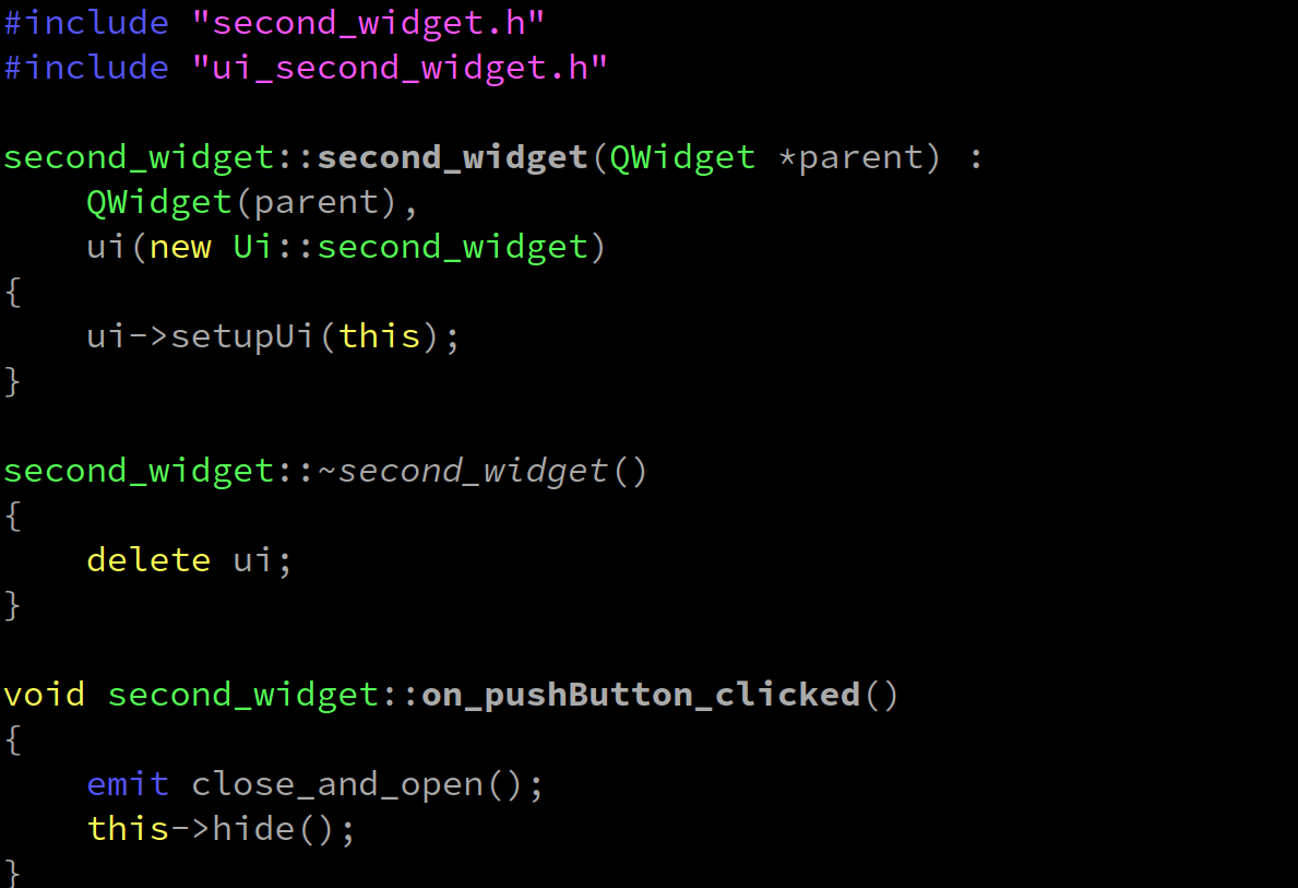
qt-C++笔记之两个窗口ui的交互
qt-C笔记之两个窗口ui的交互 code review! 文章目录 qt-C笔记之两个窗口ui的交互0.运行1.文件结构2.先创建widget项目,搞一个窗口ui出来3.项目添加第二个widget窗口出来4.补充代码4.1.qt_widget_interaction.pro4.2.main.cpp4.3.widget.h4.4.widget.cpp4.5.second…...

Redis-核心数据结构
五种数据结构 String结构 String结构应用场景 Hash结构 Hash结构应用场景 List结构 List结构应用场景 Set结构 Set结构应用场景 ZSet有序结构 ZSet有序结构应用场景...

设计模式—结构型模式之外观模式(门面模式)
设计模式—结构型模式之外观模式(门面模式) 外观(Facade)模式又叫作门面模式,是一种通过为多个复杂的子系统提供一个一致的接口,而使这些子系统更加容易被访问的模式。 例子 我们的电脑会有很多 组件&am…...

CentOS Stream 9-使用 systemd 管理自己程序时自定义日志路径
systemd 文件 [rootnode1 ~]# cat /etc/systemd/system/spms-wvp.service [Unit] DescriptionWVP service [Service] # 关键配置部分,注意这里的 spms-wvp ,后面需要用 SyslogIdentifierspms-wvp StandardOutputsyslog StandardErrorsyslog Typesimple Environment…...

动态页面调研及设计方案
文章目录 vue2 动态表单、动态页面调研一、form-generator二、ng-form-element三、Variant Form四、form-create vue2 动态表单、动态页面调研 一、form-generator 预览:https://mrhj.gitee.io/form-generator/#/ Vue2 Element UI支持拖拽生成表单不支持其他组件…...

鸿蒙4.0开发笔记之DevEco Studio之配置代码片段快速生成(三)
一、作用 配置代码片段可以让我们在Deveco Studio中进行开发时快速调取常用的代码块、字符串或者某段具有特殊含义的文字。其实现方式类似于调用定义好变量,然而这个变量是存在于Deveco Studio中的,并不会占用项目的资源。 二、配置代码段的方法 1、打…...

HarmonyOS真机调试报错:INSTALL_PARSE_FAILED_USESDK_ERROR处理
文章目录 1、 新建应用时选择与自己真机匹配的sdk版本2、 根据报错提示连接打开处理方案3、查询真机版本对应的**compileSdkVersion** 和 **compatibleSdkVersion** 提示3.1版本之后和3.1版本之前的不同命令(此处为3.0版本)4、根据查询修改参数5、连接成…...

webSocket基于面向对象二次封装
今天不睡,熬夜赶了个WebSocket 二次封装,也对这几天文章摸鱼感到抱歉,所以我出了一个注释非常非常全的代码 思路如下 首先,需要通过调用connect方法来建立WebSocket连接。当连接成功时,会调用我提供的回调函数,并将连接成功的消息帧作为参数…...

<el-button type=“primary“><el-icon><Plus /></el-icon> 上传照片</el-button>的庖丁解牛
它的本质是:**这行代码不仅仅是一个按钮,它是一个 复合交互单元 (Composite Interaction Unit)。它通过 语义化标签 (el-button)、视觉信号 (type"primary", Plus Icon) 和 文本提示 (“上传照片”) 的组合,向用户传达了一个明确的…...

为什么你的学术论文需要APA第7版样式表?3分钟解决Word格式难题
为什么你的学术论文需要APA第7版样式表?3分钟解决Word格式难题 【免费下载链接】APA-7th-Edition Microsoft Word XSD for generating APA 7th edition references 项目地址: https://gitcode.com/gh_mirrors/ap/APA-7th-Edition 作为一名学术研究者或学生&a…...

LABVIEW生成EXE
遇到的问题报错说找不到这个路径的某个VI原因在于之前手动改过文件夹名称,导致路径有变更。更关键的是有的VI还沿用以前旧的路径,因此报错。解决办法就是打开可能用到这个功能的VI,选定新路径。报错是因为要打包的vi里面不是所有的vi都能够正…...

三分钟永久备份你的QQ空间:告别数据丢失的终极解决方案
三分钟永久备份你的QQ空间:告别数据丢失的终极解决方案 【免费下载链接】QZoneExport QQ空间导出助手,用于备份QQ空间的说说、日志、私密日记、相册、视频、留言板、QQ好友、收藏夹、分享、最近访客为文件,便于迁移与保存 项目地址: https:…...

ElegantBook终极指南:5分钟学会专业书籍排版,告别格式烦恼
ElegantBook终极指南:5分钟学会专业书籍排版,告别格式烦恼 【免费下载链接】ElegantBook Elegant LaTeX Template for Books 项目地址: https://gitcode.com/gh_mirrors/el/ElegantBook 你是否曾经为学术论文或专业书籍的排版而烦恼?复…...

STM32 HAL库驱动DS18B20避坑指南:单总线时序不准?试试用定时器精准延时
STM32 HAL库驱动DS18B20避坑指南:单总线时序不准?试试用定时器精准延时 在嵌入式开发中,温度传感器DS18B20因其单总线接口和数字输出特性广受欢迎。然而,许多开发者在使用STM32 HAL库驱动DS18B20时,常遇到温度读取失败…...

路由算法的终极真相:为何“绝对最佳”是伪命题?从理论陷阱到工程实战的深度破局
路由算法的终极真相:为何“绝对最佳”是伪命题?从理论陷阱到工程实战的深度破局 摘要:在计算机网络的浩瀚星图中,路由选择算法如同指引数据包穿越迷雾的灯塔。然而,无数工程师和架构师曾陷入一个巨大的思维误区&#x…...
工作流)
LangGraph 实战:如何实现 Human-in-the-Loop(人机协同)工作流
LangGraph实战:从零构建生产级Human-in-the-Loop人机协同工作流 副标题:含中断/人工审核/分支路由全场景实现,覆盖金融/法律/企业服务90%+通用场景 第一部分:引言与基础 1.1 摘要/引言 你有没有遇到过这些场景: 用大模型做合同自动审核,结果模型漏判了关键合规条款,直…...

机器学习的几何本质:形状、距离与意义的三层重构
1. 这不是数学课,而是一场关于“机器如何看懂世界”的底层解剖你有没有想过,当一台机器识别出照片里是一只猫,它到底“看见”了什么?不是毛色、不是胡须、不是圆眼睛——它看见的是一组高维空间里的点云分布,是这些点之…...

TikTok广告账号被封怎么解决?2026年防封号完整攻略
做TikTok广告投放,最让人头疼的事情是什么?账号被封。前一秒还在跑量,后一秒突然提示账号异常,所有广告计划全部暂停,预算打水漂,客户推广计划全乱。这种经历,做过TikTok广告投放的卖家应该都不…...