[足式机器人]Part3 机构运动学与动力学分析与建模 Ch00-1 坐标系与概念基准
本文仅供学习使用,总结很多本现有讲述运动学或动力学书籍后的总结,从矢量的角度进行分析,方法比较传统,但更易理解,并且现有的看似抽象方法,两者本质上并无不同。
2024年底本人学位论文发表后方可摘抄
若有帮助请引用
本文参考:
食用方法
坐标系的组成与表达方式
点的运动在不同三维坐标系中的表达与运动描述——推导的过程?
广义坐标系的推广
点的表达与向量表达,及其不同点(投影矩阵的作用?)
建议把每个图自己都画一遍,理解每个符号表达的含义,以及为什么这么表达(尤其是如何定义角度、向量)
机构运动学与动力学分析与建模 Ch00-1 坐标系与概念基准
- 1. 空间坐标系
- 1.1 笛卡尔坐标系 Cartesian coordinate system
- 1.2 点Partical的运动与表达
- 1.2.1 笛卡尔直角坐标系
- 1.2.2 笛卡尔柱坐标系
- 1.2.3 笛卡尔球坐标系
- 1.2.4 曲线坐标系:Frenet标架(详见微分几何-曲线论内容)
- 1.2.5 广义坐标系 Generalized coordinates system
- 1.3 矢量Vector在坐标系下的表示与关系转换
1. 空间坐标系
坐标系Coordinates是一个用于描述 n n n维系统中某一状态参数的坐标表示系统:对于同一 n n n维系统的状态参数可用不同的坐标系进行表示,即具有不同的 基底Basis(基矢量) ;而对于不同的坐标系而言,表示同一状态参数存在对应关系,因此坐标系之间也存在着 变化关系,这种变化关系的本质是不同坐标系的基底之间的转换。
-
坐标系的表达: { F } \left\{ F \right\} {F}, { M } \left\{ M \right\} {M},其中“ { } \{\} {}”符号特指坐标系,一般用 { F } \left\{ F \right\} {F}表示
固定坐标系 Fixed, { M } \left\{ M \right\} {M}表示运动坐标系 Moving;对于部分坐标系也可以称为标架Frame。 -
基矢量的表达: i ^ , j ^ , k ^ \hat{i},\hat{j},\hat{k} i^,j^,k^,其中 “ ^ \hat{ } ^ ” 符号特指基矢量;对于固定坐标系 { F } \left\{ F \right\} {F},其基矢量特定为: I ^ , J ^ , K ^ \hat{I},\hat{J},\hat{K} I^,J^,K^,对于其他运动坐标系而言,以坐标系 { M } \left\{ M \right\} {M}为例,其基矢量可写成: i ^ M , j ^ M , k ^ M \hat{i}^M,\hat{j}^M,\hat{k}^M i^M,j^M,k^M
-
标架的表达:以 { M } \left\{ M \right\} {M}为例,其运动标架可表示为: { M : ( i ^ M , j ^ M , k ^ M ) } \left\{ M:\left( \hat{i}^M,\hat{j}^M,\hat{k}^M \right) \right\} {M:(i^M,j^M,k^M)}
当坐标系的维数 n = 3 n=3 n=3 时,便称为空间坐标系。
1.1 笛卡尔坐标系 Cartesian coordinate system
笛卡尔坐标系是我们在三维空间中常用的表示空间运动的坐标系,基于观测位置与对象的不同,还有GPS坐标系 等其他表达方式。对于任一笛卡尔坐标系,视其基矢量为 X ^ 1 , X ^ 2 , X ^ 3 \hat{X}_1,\hat{X}_2,\hat{X}_3 X^1,X^2,X^3,对于该空间内任一点 P P P 都可以这组基矢量进行表达。
1.2 点Partical的运动与表达
对于空间中任意一点 P P P而言,其位置Position表述该系统空间的一种状态参数,因此其在各基矢量上的标量分量即为对应的坐标参数。因此该点 P P P在笛卡尔坐标系中的表达为:
R ⃗ P X = P ⃗ = P 1 X ^ 1 + P 2 X ^ 2 + P 3 X ^ 3 \vec{R}_{\mathrm{P}}^{X}=\vec{P}=P_1\hat{X}_1+P_2\hat{X}_2+P_3\hat{X}_3 RPX=P=P1X^1+P2X^2+P3X^3
1.2.1 笛卡尔直角坐标系
{ F : ( X ^ 1 , X ^ 2 , X ^ 3 ) } = { F : ( I ^ , J ^ , K ^ ) } \left\{ F:\left( \hat{X}_1,\hat{X}_2,\hat{X}_3 \right) \right\} =\left\{ F:\left( \hat{I},\hat{J},\hat{K} \right) \right\} {F:(X^1,X^2,X^3)}={F:(I^,J^,K^)}

对于状态空间中一点 P P P,其在固定坐标系标架 { F : ( I ^ , J ^ , K ^ ) } \left\{ F:\left( \hat{I},\hat{J},\hat{K} \right) \right\} {F:(I^,J^,K^)}上基矢量的投影参数为 ( P 1 , P 2 , P 3 ) \left( P_1,P_2,P_3 \right) (P1,P2,P3),因此可将点 P P P 在笛卡尔直角坐标系中进行表述
R ⃗ P F = P 1 I ^ + P 2 J ^ + P 3 K ^ = [ I ^ J ^ K ^ ] T [ P 1 P 2 P 3 ] \vec{R}_{\mathrm{P}}^{F}=P_1\hat{I}+P_2\hat{J}+P_3\hat{K}=\left[ \begin{array}{c} \hat{I}\\ \hat{J}\\ \hat{K}\\ \end{array} \right] ^{\mathrm{T}}\left[ \begin{array}{c} P_1\\ P_2\\ P_3\\ \end{array} \right] RPF=P1I^+P2J^+P3K^= I^J^K^ T P1P2P3
进而可以求解其速度Velocity参数 V ⃗ P F \vec{V}_{\mathrm{P}}^{F} VPF 为:
V ⃗ P F = R ⃗ ˙ P F = d R ⃗ P F d t = [ I ^ ˙ ↗ 0 J ^ ˙ ↗ 0 K ^ ˙ ↗ 0 ] T [ P 1 P 2 P 3 ] + [ I ^ J ^ K ^ ] T [ P ˙ 1 P ˙ 2 P ˙ 3 ] \vec{V}_{\mathrm{P}}^{F}=\dot{\vec{R}}_{\mathrm{P}}^{F}=\frac{\mathrm{d}\vec{R}_{\mathrm{P}}^{F}}{\mathrm{dt}}=\left[ \begin{array}{c} \dot{\hat{I}}_{\nearrow 0}\\ \dot{\hat{J}}_{\nearrow 0}\\ \dot{\hat{K}}_{\nearrow 0}\\ \end{array} \right] ^{\mathrm{T}}\left[ \begin{array}{c} P_1\\ P_2\\ P_3\\ \end{array} \right] +\left[ \begin{array}{c} \hat{I}\\ \hat{J}\\ \hat{K}\\ \end{array} \right] ^{\mathrm{T}}\left[ \begin{array}{c} \dot{P}_1\\ \dot{P}_2\\ \dot{P}_3\\ \end{array} \right] VPF=R˙PF=dtdRPF= I^˙↗0J^˙↗0K^˙↗0 T P1P2P3 + I^J^K^ T P˙1P˙2P˙3
其加速度acceleration参数 a ⃗ P F \vec{a}_{\mathrm{P}}^{F} aPF 为:
a ⃗ P F = V ⃗ ˙ P F = R ⃗ ¨ P F = d V ⃗ P F d t = [ I ^ ˙ ↗ 0 J ^ ˙ ↗ 0 K ^ ˙ ↗ 0 ] T [ P ˙ 1 P ˙ 2 P ˙ 3 ] + [ I ^ J ^ K ^ ] T [ P ¨ 1 P ¨ 2 P ¨ 3 ] \vec{a}_{\mathrm{P}}^{F}=\dot{\vec{V}}_{\mathrm{P}}^{F}=\ddot{\vec{R}}_{\mathrm{P}}^{F}=\frac{\mathrm{d}\vec{V}_{\mathrm{P}}^{F}}{\mathrm{dt}}=\left[ \begin{array}{c} \dot{\hat{I}}_{\nearrow 0}\\ \dot{\hat{J}}_{\nearrow 0}\\ \dot{\hat{K}}_{\nearrow 0}\\ \end{array} \right] ^{\mathrm{T}}\left[ \begin{array}{c} \dot{P}_1\\ \dot{P}_2\\ \dot{P}_3\\ \end{array} \right] +\left[ \begin{array}{c} \hat{I}\\ \hat{J}\\ \hat{K}\\ \end{array} \right] ^{\mathrm{T}}\left[ \begin{array}{c} \ddot{P}_1\\ \ddot{P}_2\\ \ddot{P}_3\\ \end{array} \right] aPF=V˙PF=R¨PF=dtdVPF= I^˙↗0J^˙↗0K^˙↗0 T P˙1P˙2P˙3 + I^J^K^ T P¨1P¨2P¨3
1.2.2 笛卡尔柱坐标系
{ F : ( X ^ 1 , X ^ 2 , X ^ 3 ) } = { F : ( X ^ r , X ^ θ , K ^ ) } \left\{ F:\left( \hat{X}_1,\hat{X}_2,\hat{X}_3 \right) \right\} =\left\{ F:\left( \hat{X}_{\mathrm{r}},\hat{X}_{\mathrm{\theta}},\hat{K} \right) \right\} {F:(X^1,X^2,X^3)}={F:(X^r,X^θ,K^)}

对于不同的坐标系,点 P P P 在状态空间中并没有发生变化,而由于基矢量的变化导致其投影参数发生改变。在柱坐标系中,点 P P P 表述为:
R ⃗ P C = P ⃗ = P 1 ′ X ^ r + P 2 ′ X ^ θ + P 3 ′ K ^ \vec{R}_{\mathrm{P}}^{\mathrm{C}}=\vec{P}=P_1\mathrm{'}\hat{X}_{\mathrm{r}}+P_2\mathrm{'}\hat{X}_{\theta}+P_3\mathrm{'}\hat{K} RPC=P=P1′X^r+P2′X^θ+P3′K^
对于投影参数而言, P 1 ′ P_1\mathrm{'} P1′表示 X ^ r \hat{X}_{\mathrm{r}} X^r方向上的长度参数,而 P 2 ′ P_2\mathrm{'} P2′表示 X ^ θ \hat{X}_{\mathrm{\theta}} X^θ方向上的角度参数,而单纯的角度参数在实际的矢量运算过程中是比较难于理解的,因此对柱坐标系而言,实际上是将该方向上的已知投影参数转换到直角坐标系下进行表示
若已知柱坐标系下点 P P P 的投影参数 P = ( r , θ , k ) P=\left( r,\theta ,k \right) P=(r,θ,k),其位置方程在直角坐标系下的表示为:
R ⃗ P F = P ⃗ = r cos θ I ^ + r sin θ J ^ + k K ^ \vec{R}_{\mathrm{P}}^{\mathrm{F}}=\vec{P}=r\cos \theta \hat{I}+r\sin \theta \hat{J}+k\hat{K} RPF=P=rcosθI^+rsinθJ^+kK^
可视为: [ P 1 P 2 P 3 ] = [ r cos θ r sin θ k ] \left[ \begin{array}{c} P_1\\ P_2\\ P_3\\ \end{array} \right] =\left[ \begin{array}{c} r\cos \theta\\ r\sin \theta\\ k\\ \end{array} \right] P1P2P3 = rcosθrsinθk ,对速度参数 V ⃗ P C \vec{V}_{\mathrm{P}}^{\mathrm{C}} VPC进行求解:
V ⃗ P F = R ⃗ ˙ P F = d R ⃗ P F d t = [ I ^ J ^ K ^ ] T [ P ˙ 1 P ˙ 2 P ˙ 3 ] = [ I ^ J ^ K ^ ] T [ d r d t cos θ − r d θ d t sin θ d r d t sin θ + r d θ d t cos θ d k d t ] \vec{V}_{\mathrm{P}}^{\mathrm{F}}=\dot{\vec{R}}_{\mathrm{P}}^{\mathrm{F}}=\frac{\mathrm{d}\vec{R}_{\mathrm{P}}^{\mathrm{F}}}{\mathrm{dt}}=\left[ \begin{array}{c} \hat{I}\\ \hat{J}\\ \hat{K}\\ \end{array} \right] ^{\mathrm{T}}\left[ \begin{array}{c} \dot{P}_1\\ \dot{P}_2\\ \dot{P}_3\\ \end{array} \right] =\left[ \begin{array}{c} \hat{I}\\ \hat{J}\\ \hat{K}\\ \end{array} \right] ^{\mathrm{T}}\left[ \begin{array}{c} \frac{\mathrm{d}r}{\mathrm{dt}}\cos \theta -r\frac{\mathrm{d}\theta}{\mathrm{dt}}\sin \theta\\ \frac{\mathrm{d}r}{\mathrm{dt}}\sin \theta +r\frac{\mathrm{d}\theta}{\mathrm{dt}}\cos \theta\\ \frac{\mathrm{d}k}{\mathrm{dt}}\\ \end{array} \right] VPF=R˙PF=dtdRPF= I^J^K^ T P˙1P˙2P˙3 = I^J^K^ T dtdrcosθ−rdtdθsinθdtdrsinθ+rdtdθcosθdtdk
当 d r d t = 0 \frac{\mathrm{d}r}{\mathrm{dt}}=0 dtdr=0, d k d t = 0 \frac{\mathrm{d}k}{\mathrm{dt}}=0 dtdk=0 时,即点 P P P 不在矢径方向上运动,仅绕 K ^ \hat{K} K^ 进行平面上的纯回转,可将上式简化为:
V ⃗ P F ∣ d r d t = 0 , d k d t = 0 = [ I ^ J ^ K ^ ] T [ − r d θ d t sin θ r d θ d t cos θ 0 ] = r θ ˙ [ I ^ J ^ K ^ ] T [ − sin θ cos θ 0 ] \left. \vec{V}_{\mathrm{P}}^{\mathrm{F}} \right|_{\frac{\mathrm{d}r}{\mathrm{dt}}=0,\frac{\mathrm{d}k}{\mathrm{dt}}=0}=\left[ \begin{array}{c} \hat{I}\\ \hat{J}\\ \hat{K}\\ \end{array} \right] ^{\mathrm{T}}\left[ \begin{array}{c} -r\frac{\mathrm{d}\theta}{\mathrm{dt}}\sin \theta\\ r\frac{\mathrm{d}\theta}{\mathrm{dt}}\cos \theta\\ 0\\ \end{array} \right] =r\dot{\theta}\left[ \begin{array}{c} \hat{I}\\ \hat{J}\\ \hat{K}\\ \end{array} \right] ^{\mathrm{T}}\left[ \begin{array}{c} -\sin \theta\\ \cos \theta\\ 0\\ \end{array} \right] VPF dtdr=0,dtdk=0= I^J^K^ T −rdtdθsinθrdtdθcosθ0 =rθ˙ I^J^K^ T −sinθcosθ0
对上式进一步求解其加速度参数 a ⃗ P F ∣ d r d t = 0 , d k d t = 0 \left. \vec{a}_{\mathrm{P}}^{\mathrm{F}} \right|_{\frac{\mathrm{d}r}{\mathrm{dt}}=0,\frac{\mathrm{d}k}{\mathrm{dt}}=0} aPF dtdr=0,dtdk=0:
a ⃗ P F ∣ d r d t = 0 , d k d t = 0 = r θ ¨ [ I ^ J ^ K ^ ] T [ − sin θ cos θ 0 ] + r θ ˙ 2 [ I ^ J ^ K ^ ] T [ − cos θ − sin θ 0 ] = α ⃗ F × R ⃗ P F + ω ⃗ F × V ⃗ P F \left. \vec{a}_{\mathrm{P}}^{\mathrm{F}} \right|_{\frac{\mathrm{d}r}{\mathrm{dt}}=0,\frac{\mathrm{d}k}{\mathrm{dt}}=0}=r\ddot{\theta}\left[ \begin{array}{c} \hat{I}\\ \hat{J}\\ \hat{K}\\ \end{array} \right] ^{\mathrm{T}}\left[ \begin{array}{c} -\sin \theta\\ \cos \theta\\ 0\\ \end{array} \right] +r\dot{\theta}^2\left[ \begin{array}{c} \hat{I}\\ \hat{J}\\ \hat{K}\\ \end{array} \right] ^{\mathrm{T}}\left[ \begin{array}{c} -\cos \theta\\ -\sin \theta\\ 0\\ \end{array} \right] =\vec{\alpha}^{\mathrm{F}}\times \vec{R}_{\mathrm{P}}^{\mathrm{F}}+\vec{\omega}^{\mathrm{F}}\times \vec{V}_{\mathrm{P}}^{\mathrm{F}} aPF dtdr=0,dtdk=0=rθ¨ I^J^K^ T −sinθcosθ0 +rθ˙2 I^J^K^ T −cosθ−sinθ0 =αF×RPF+ωF×VPF
若考虑真实的向量表达,则柱坐标系中,点 P P P 还可以表述为:
R ⃗ P C = r ( θ ) X ^ r ( θ ) + k K ^ \vec{R}_{\mathrm{P}}^{\mathrm{C}}=r\left( \theta \right) \hat{X}_{\mathrm{r}\left( \theta \right)}+k\hat{K} RPC=r(θ)X^r(θ)+kK^
其中:
[ X ^ r X ^ θ ] = [ cos θ sin θ − sin θ cos θ ] [ I ^ J ^ ] \left[ \begin{array}{c} \hat{X}_{\mathrm{r}}\\ \hat{X}_{\mathrm{\theta}}\\ \end{array} \right] =\left[ \begin{matrix} \cos \theta& \sin \theta\\ -\sin \theta& \cos \theta\\ \end{matrix} \right] \left[ \begin{array}{c} \hat{I}\\ \hat{J}\\ \end{array} \right] [X^rX^θ]=[cosθ−sinθsinθcosθ][I^J^]
进而可得:
[ X ^ ˙ r X ^ ˙ θ ] = [ − θ ˙ sin θ θ ˙ cos θ − θ ˙ cos θ − θ ˙ sin θ ] [ I ^ J ^ ] = [ 0 θ ˙ − θ ˙ 0 ] [ X ^ r X ^ θ ] \left[ \begin{array}{c} \dot{\hat{X}}_{\mathrm{r}}\\ \dot{\hat{X}}_{\mathrm{\theta}}\\ \end{array} \right] =\left[ \begin{matrix} -\dot{\theta}\sin \theta& \dot{\theta}\cos \theta\\ -\dot{\theta}\cos \theta& -\dot{\theta}\sin \theta\\ \end{matrix} \right] \left[ \begin{array}{c} \hat{I}\\ \hat{J}\\ \end{array} \right] =\left[ \begin{matrix} 0& \dot{\theta}\\ -\dot{\theta}& 0\\ \end{matrix} \right] \left[ \begin{array}{c} \hat{X}_{\mathrm{r}}\\ \hat{X}_{\mathrm{\theta}}\\ \end{array} \right] [X^˙rX^˙θ]=[−θ˙sinθ−θ˙cosθθ˙cosθ−θ˙sinθ][I^J^]=[0−θ˙θ˙0][X^rX^θ]
对于 X ^ r \hat{X}_{\mathrm{r}} X^r与 X ^ θ \hat{X}_{\theta} X^θ而言有: X ^ ˙ r = θ ˙ X ^ θ , X ^ θ = − θ ˙ X ^ ˙ r \dot{\hat{X}}_{\mathrm{r}}=\dot{\theta}\hat{X}_{\theta},\hat{X}_{\theta}=-\dot{\theta}\dot{\hat{X}}_{\mathrm{r}} X^˙r=θ˙X^θ,X^θ=−θ˙X^˙r,此处的 X ^ θ \hat{X}_{\theta} X^θ表示的是垂直于基矢量 X ^ r \hat{X}_{\mathrm{r}} X^r的切矢量,与 X ^ θ \hat{X}_{\theta} X^θ不同。
虽然在三维系统中正常应该具有三个基矢量,而在上式中只有两个基矢量,但其投影参数与矢径上的基矢量为另一个参数 θ \theta θ的函数,因此该式为真实表达形式,同样可得其速度与加速度参数为:
{ V ⃗ P C = R ⃗ ˙ P C = r ˙ X ^ r + r X ^ ˙ r + k ˙ K ^ = r ˙ X ^ r + r θ ˙ X ^ θ + k ˙ K ^ a ⃗ P C = V ⃗ ˙ P C = r ¨ X ^ r + r ˙ X ^ ˙ r + r ˙ θ ˙ X ^ θ + r θ ¨ X ^ θ + r θ ˙ X ^ ˙ θ + k ¨ K ^ = r ¨ X ^ r + r ˙ θ ˙ X ^ θ + r ˙ θ ˙ X ^ θ + r θ ¨ X ^ θ − r θ ˙ 2 X ^ r + k ¨ K ^ \left\{ \begin{array}{c} \vec{V}_{\mathrm{P}}^{\mathrm{C}}=\dot{\vec{R}}_{\mathrm{P}}^{\mathrm{C}}=\dot{r}\hat{X}_{\mathrm{r}}+r\dot{\hat{X}}_{\mathrm{r}}+\dot{k}\hat{K}=\dot{r}\hat{X}_{\mathrm{r}}+r\dot{\theta}\hat{X}_{\mathrm{\theta}}+\dot{k}\hat{K}\\ \vec{a}_{\mathrm{P}}^{\mathrm{C}}=\dot{\vec{V}}_{\mathrm{P}}^{\mathrm{C}}=\ddot{r}\hat{X}_{\mathrm{r}}+\dot{r}\dot{\hat{X}}_{\mathrm{r}}+\dot{r}\dot{\theta}\hat{X}_{\mathrm{\theta}}+r\ddot{\theta}\hat{X}_{\mathrm{\theta}}+r\dot{\theta}\dot{\hat{X}}_{\mathrm{\theta}}+\ddot{k}\hat{K}=\ddot{r}\hat{X}_{\mathrm{r}}+\dot{r}\dot{\theta}\hat{X}_{\mathrm{\theta}}+\dot{r}\dot{\theta}\hat{X}_{\mathrm{\theta}}+r\ddot{\theta}\hat{X}_{\mathrm{\theta}}-r\dot{\theta}^2\hat{X}_{\mathrm{r}}+\ddot{k}\hat{K}\\ \end{array} \right. ⎩ ⎨ ⎧VPC=R˙PC=r˙X^r+rX^˙r+k˙K^=r˙X^r+rθ˙X^θ+k˙K^aPC=V˙PC=r¨X^r+r˙X^˙r+r˙θ˙X^θ+rθ¨X^θ+rθ˙X^˙θ+k¨K^=r¨X^r+r˙θ˙X^θ+r˙θ˙X^θ+rθ¨X^θ−rθ˙2X^r+k¨K^
对上式)进行化简,可得:
{ V ⃗ P C = r ˙ X ^ r + r θ ˙ X ^ θ + k ˙ K ^ a ⃗ P C = ( r ¨ − r θ ˙ 2 ) X ^ r + ( 2 r ˙ θ ˙ + r θ ¨ ) X ^ θ + k ¨ K ^ \left\{ \begin{array}{c} \vec{V}_{\mathrm{P}}^{\mathrm{C}}=\dot{r}\hat{X}_{\mathrm{r}}+r\dot{\theta}\hat{X}_{\theta}+\dot{k}\hat{K}\\ \vec{a}_{\mathrm{P}}^{\mathrm{C}}=\left( \ddot{r}-r\dot{\theta}^2 \right) \hat{X}_{\mathrm{r}}+\left( 2\dot{r}\dot{\theta}+r\ddot{\theta} \right) \hat{X}_{\theta}+\ddot{k}\hat{K}\\ \end{array} \right. {VPC=r˙X^r+rθ˙X^θ+k˙K^aPC=(r¨−rθ˙2)X^r+(2r˙θ˙+rθ¨)X^θ+k¨K^
其中: r θ ¨ r\ddot{\theta} rθ¨ 称为欧拉项Eulerian term, 2 r ˙ θ ˙ 2\dot{r}\dot{\theta} 2r˙θ˙ 称为科里奥利项Coriolis term。
1.2.3 笛卡尔球坐标系
{ F : ( X ^ 1 , X ^ 2 , X ^ 3 ) } = { F : ( X ^ r , X ^ θ , X ^ ϕ ) } \left\{ F:\left( \hat{X}_1,\hat{X}_2,\hat{X}_3 \right) \right\} =\left\{ F:\left( \hat{X}_{\mathrm{r}},\hat{X}_{\mathrm{\theta}},\hat{X}_{\mathrm{\phi}} \right) \right\} {F:(X^1,X^2,X^3)}={F:(X^r,X^θ,X^ϕ)}

笛卡尔球坐标系也可以基于投影参数 P = ( r , θ , ϕ ) P=\left( r,\theta ,\mathrm{\phi} \right) P=(r,θ,ϕ) 在直角坐标系中进行表达,则点 P P P 的运动参数为:
R ⃗ P F = [ I ^ J ^ K ^ ] T [ r sin ϕ cos θ r sin ϕ sin θ r cos ϕ ] \vec{R}_{\mathrm{P}}^{F}=\left[ \begin{array}{c} \hat{I}\\ \hat{J}\\ \hat{K}\\ \end{array} \right] ^{\mathrm{T}}\left[ \begin{array}{c} r\sin \phi \cos \theta\\ r\sin \phi \sin \theta\\ r\cos \phi\\ \end{array} \right] RPF= I^J^K^ T rsinϕcosθrsinϕsinθrcosϕ
V ⃗ P F = [ I ^ J ^ K ^ ] T [ r ˙ sin ϕ cos θ + r ϕ ˙ cos ϕ cos θ − r θ ˙ sin ϕ sin θ r ˙ sin ϕ sin θ + r ϕ ˙ cos ϕ sin θ + r θ ˙ sin ϕ cos θ r ˙ cos ϕ − r ϕ ˙ sin ϕ ] \vec{V}_{\mathrm{P}}^{F}=\left[ \begin{array}{c} \hat{I}\\ \hat{J}\\ \hat{K}\\ \end{array} \right] ^{\mathrm{T}}\left[ \begin{array}{c} \dot{r}\sin \phi \cos \theta +r\dot{\phi}\cos \phi \cos \theta -r\dot{\theta}\sin \phi \sin \theta\\ \dot{r}\sin \phi \sin \theta +r\dot{\phi}\cos \phi \sin \theta +r\dot{\theta}\sin \phi \cos \theta\\ \dot{r}\cos \phi -r\dot{\phi}\sin \phi\\ \end{array} \right] VPF= I^J^K^ T r˙sinϕcosθ+rϕ˙cosϕcosθ−rθ˙sinϕsinθr˙sinϕsinθ+rϕ˙cosϕsinθ+rθ˙sinϕcosθr˙cosϕ−rϕ˙sinϕ
a ⃗ P F = [ I ^ J ^ K ^ ] T [ ( r ¨ − r ϕ ˙ 2 − r θ ˙ 2 ) sin ϕ cos θ + ( 2 r ˙ ϕ ˙ + r ϕ ¨ ) cos ϕ cos θ − ( 2 r ˙ θ ˙ + r θ ¨ ) sin ϕ sin θ − ( 2 r θ ˙ ϕ ˙ ) cos ϕ sin θ ( r ¨ − r ϕ ˙ 2 − r θ ˙ 2 ) sin ϕ sin θ + ( 2 r ˙ ϕ ˙ + r ϕ ¨ ) cos ϕ sin θ + ( 2 r ˙ θ ˙ + r θ ¨ ) sin ϕ cos θ + ( 2 r θ ˙ ϕ ˙ ) cos ϕ cos θ ( r ¨ − r ϕ ˙ 2 ) cos ϕ − ( 2 r ˙ ϕ ˙ + r ϕ ¨ ) sin ϕ ] \vec{a}_{\mathrm{P}}^{F}=\left[ \begin{array}{c} \hat{I}\\ \hat{J}\\ \hat{K}\\ \end{array} \right] ^{\mathrm{T}}\left[ \begin{array}{c} \left( \ddot{r}-r\dot{\phi}^2-r\dot{\theta}^2 \right) \sin \phi \cos \theta +\left( 2\dot{r}\dot{\phi}+r\ddot{\phi} \right) \cos \phi \cos \theta -\left( 2\dot{r}\dot{\theta}+r\ddot{\theta} \right) \sin \phi \sin \theta -\left( 2r\dot{\theta}\dot{\phi} \right) \cos \phi \sin \theta\\ \left( \ddot{r}-r\dot{\phi}^2-r\dot{\theta}^2 \right) \sin \phi \sin \theta +\left( 2\dot{r}\dot{\phi}+r\ddot{\phi} \right) \cos \phi \sin \theta +\left( 2\dot{r}\dot{\theta}+r\ddot{\theta} \right) \sin \phi \cos \theta +\left( 2r\dot{\theta}\dot{\phi} \right) \cos \phi \cos \theta\\ \left( \ddot{r}-r\dot{\phi}^2 \right) \cos \phi -\left( 2\dot{r}\dot{\phi}+r\ddot{\phi} \right) \sin \phi\\ \end{array} \right] aPF= I^J^K^ T (r¨−rϕ˙2−rθ˙2)sinϕcosθ+(2r˙ϕ˙+rϕ¨)cosϕcosθ−(2r˙θ˙+rθ¨)sinϕsinθ−(2rθ˙ϕ˙)cosϕsinθ(r¨−rϕ˙2−rθ˙2)sinϕsinθ+(2r˙ϕ˙+rϕ¨)cosϕsinθ+(2r˙θ˙+rθ¨)sinϕcosθ+(2rθ˙ϕ˙)cosϕcosθ(r¨−rϕ˙2)cosϕ−(2r˙ϕ˙+rϕ¨)sinϕ
在笛卡尔球坐标中,如图所示,可将点 P P P 的位置表述为:
R ⃗ p s = r X ^ r \vec{R}_{\mathrm{p}}^{s}=r\hat{X}_{\mathrm{r}} Rps=rX^r
其中:
[ X ^ ϕ X ^ θ X ^ r ] = [ cos ϕ cos θ cos ϕ sin θ − sin ϕ − sin θ cos θ 0 sin ϕ cos θ sin ϕ sin θ cos ϕ ] [ I ^ J ^ K ^ ] \left[ \begin{array}{c} \hat{X}_{\mathrm{\phi}}\\ \hat{X}_{\mathrm{\theta}}\\ \hat{X}_{\mathrm{r}}\\ \end{array} \right] =\left[ \begin{matrix} \cos \phi \cos \theta& \cos \phi \sin \theta& -\sin \phi\\ -\sin \theta& \cos \theta& 0\\ \sin \phi \cos \theta& \sin \phi \sin \theta& \cos \phi\\ \end{matrix} \right] \left[ \begin{array}{c} \hat{I}\\ \hat{J}\\ \hat{K}\\ \end{array} \right] X^ϕX^θX^r = cosϕcosθ−sinθsinϕcosθcosϕsinθcosθsinϕsinθ−sinϕ0cosϕ I^J^K^
进而求得:
[ X ^ ˙ ϕ X ^ ˙ θ X ^ ˙ r ] = [ − ϕ ˙ sin ϕ cos θ − θ ˙ cos ϕ sin θ − ϕ ˙ sin ϕ sin θ + θ ˙ cos ϕ cos θ − ϕ ˙ cos ϕ − θ ˙ cos θ − θ ˙ sin θ 0 ϕ ˙ cos ϕ cos θ − θ ˙ sin ϕ sin θ ϕ ˙ cos ϕ sin θ + θ ˙ sin ϕ cos θ − ϕ ˙ sin ϕ ] [ I ^ J ^ K ^ ] = [ 0 θ ˙ cos ϕ − ϕ ˙ − θ ˙ cos ϕ 0 − θ ˙ sin ϕ ϕ ˙ θ ˙ sin ϕ 0 ] [ X ^ ϕ X ^ θ X ^ r ] \begin{split} \left[ \begin{array}{c} \dot{\hat{X}}_{\mathrm{\phi}}\\ \dot{\hat{X}}_{\mathrm{\theta}}\\ \dot{\hat{X}}_{\mathrm{r}}\\ \end{array} \right] &=\left[ \begin{matrix} -\dot{\phi}\sin \phi \cos \theta -\dot{\theta}\cos \phi \sin \theta& -\dot{\phi}\sin \phi \sin \theta +\dot{\theta}\cos \phi \cos \theta& -\dot{\phi}\cos \phi\\ -\dot{\theta}\cos \theta& -\dot{\theta}\sin \theta& 0\\ \dot{\phi}\cos \phi \cos \theta -\dot{\theta}\sin \phi \sin \theta& \dot{\phi}\cos \phi \sin \theta +\dot{\theta}\sin \phi \cos \theta& -\dot{\phi}\sin \phi\\ \end{matrix} \right] \left[ \begin{array}{c} \hat{I}\\ \hat{J}\\ \hat{K}\\ \end{array} \right] \\ &=\left[ \begin{matrix} 0& \dot{\theta}\cos \phi& -\dot{\phi}\\ -\dot{\theta}\cos \phi& 0& -\dot{\theta}\sin \phi\\ \dot{\phi}& \dot{\theta}\sin \phi& 0\\ \end{matrix} \right] \left[ \begin{array}{c} \hat{X}_{\mathrm{\phi}}\\ \hat{X}_{\mathrm{\theta}}\\ \hat{X}_{\mathrm{r}}\\ \end{array} \right] \end{split} X^˙ϕX^˙θX^˙r = −ϕ˙sinϕcosθ−θ˙cosϕsinθ−θ˙cosθϕ˙cosϕcosθ−θ˙sinϕsinθ−ϕ˙sinϕsinθ+θ˙cosϕcosθ−θ˙sinθϕ˙cosϕsinθ+θ˙sinϕcosθ−ϕ˙cosϕ0−ϕ˙sinϕ I^J^K^ = 0−θ˙cosϕϕ˙θ˙cosϕ0θ˙sinϕ−ϕ˙−θ˙sinϕ0 X^ϕX^θX^r
进而求得其速度参数为:
V ⃗ P S = R ⃗ ˙ P S = r ˙ X ^ r + r X ^ ˙ r = r ˙ X ^ r + r ϕ ˙ X ^ ϕ + r θ ˙ sin ϕ X ^ θ \vec{V}_{\mathrm{P}}^{S}=\dot{\vec{R}}_{\mathrm{P}}^{S}=\dot{r}\hat{X}_{\mathrm{r}}+r\dot{\hat{X}}_{\mathrm{r}}=\dot{r}\hat{X}_{\mathrm{r}}+r\dot{\phi}\hat{X}_{\mathrm{\phi}}+r\dot{\theta}\sin \phi \hat{X}_{\mathrm{\theta}} VPS=R˙PS=r˙X^r+rX^˙r=r˙X^r+rϕ˙X^ϕ+rθ˙sinϕX^θ
角速度参数为:(仔细观察下式与投影矩阵的关系)
V ⃗ P S = ω ⃗ S × R ⃗ P S ⇒ ω ⃗ S = θ ˙ sin ϕ X ^ ϕ − θ ˙ cos ϕ X ^ r + ϕ ˙ X ^ θ \vec{V}_{\mathrm{P}}^{S}=\vec{\omega}^S\times \vec{R}_{\mathrm{P}}^{S}\Rightarrow \vec{\omega}^S=\dot{\theta}\sin \phi \hat{X}_{\mathrm{\phi}}-\dot{\theta}\cos \phi \hat{X}_{\mathrm{r}}+\dot{\phi}\hat{X}_{\mathrm{\theta}} VPS=ωS×RPS⇒ωS=θ˙sinϕX^ϕ−θ˙cosϕX^r+ϕ˙X^θ
加速度参数为:
a ⃗ P S = V ⃗ ˙ P S = { r ¨ X ^ r + r ˙ X ^ ˙ r + r ˙ ϕ ˙ X ^ ϕ + r ϕ ¨ X ^ ϕ + r ϕ X ^ ˙ ϕ + r ˙ θ ˙ sin ϕ X ^ θ + r θ ¨ sin ϕ X ^ θ + r θ ˙ ϕ ˙ cos ϕ X ^ θ + r θ ˙ sin ϕ X ^ ˙ θ = { r ¨ X ^ r + r ˙ ( ϕ ˙ X ^ ϕ + θ ˙ sin ϕ X ^ θ ) + ( r ˙ ϕ ˙ + r ϕ ¨ ) X ^ ϕ + r ϕ ( θ ˙ cos ϕ X ^ θ − ϕ ˙ X ^ r ) + ( r ˙ θ ˙ sin ϕ + r θ ¨ sin ϕ + r θ ˙ ϕ ˙ cos ϕ ) X ^ θ + r θ ˙ sin ϕ ( − θ ˙ cos ϕ X ^ ϕ − θ ˙ sin ϕ X ^ r ) = ( r ¨ − r ϕ ϕ ˙ − r θ ˙ 2 sin ϕ 2 ) X ^ r + ( 2 r ˙ ϕ ˙ + r ϕ ¨ − r θ ˙ 2 sin ϕ cos ϕ ) X ^ ϕ + [ ( 2 r ˙ θ ˙ + r θ ¨ ) sin ϕ + ( r θ ˙ ϕ ˙ + r ϕ θ ˙ ) cos ϕ ] X ^ θ \begin{split} \vec{a}_{\mathrm{P}}^{S}&=\dot{\vec{V}}_{\mathrm{P}}^{S}=\begin{cases} \ddot{r}\hat{X}_{\mathrm{r}}+\dot{r}\dot{\hat{X}}_{\mathrm{r}}+\dot{r}\dot{\phi}\hat{X}_{\mathrm{\phi}}+r\ddot{\phi}\hat{X}_{\mathrm{\phi}}+r\phi \dot{\hat{X}}_{\mathrm{\phi}}\\ +\dot{r}\dot{\theta}\sin \phi \hat{X}_{\mathrm{\theta}}+r\ddot{\theta}\sin \phi \hat{X}_{\mathrm{\theta}}+r\dot{\theta}\dot{\phi}\cos \phi \hat{X}_{\mathrm{\theta}}+r\dot{\theta}\sin \phi \dot{\hat{X}}_{\mathrm{\theta}}\\ \end{cases} \\ &=\begin{cases} \ddot{r}\hat{X}_{\mathrm{r}}+\dot{r}\left( \dot{\phi}\hat{X}_{\mathrm{\phi}}+\dot{\theta}\sin \phi \hat{X}_{\mathrm{\theta}} \right) +\left( \dot{r}\dot{\phi}+r\ddot{\phi} \right) \hat{X}_{\mathrm{\phi}}+r\phi \left( \dot{\theta}\cos \phi \hat{X}_{\mathrm{\theta}}-\dot{\phi}\hat{X}_{\mathrm{r}} \right)\\ +\left( \dot{r}\dot{\theta}\sin \phi +r\ddot{\theta}\sin \phi +r\dot{\theta}\dot{\phi}\cos \phi \right) \hat{X}_{\mathrm{\theta}}+r\dot{\theta}\sin \phi \left( -\dot{\theta}\cos \phi \hat{X}_{\mathrm{\phi}}-\dot{\theta}\sin \phi \hat{X}_{\mathrm{r}} \right)\\ \end{cases} \\ &=\left( \ddot{r}-r\phi \dot{\phi}-r\dot{\theta}^2\sin \phi ^2 \right) \hat{X}_{\mathrm{r}}+\left( 2\dot{r}\dot{\phi}+r\ddot{\phi}-r\dot{\theta}^2\sin \phi \cos \phi \right) \hat{X}_{\mathrm{\phi}}+\left[ \left( 2\dot{r}\dot{\theta}+r\ddot{\theta} \right) \sin \phi +\left( r\dot{\theta}\dot{\phi}+r\phi \dot{\theta} \right) \cos \phi \right] \hat{X}_{\mathrm{\theta}} \end{split} aPS=V˙PS={r¨X^r+r˙X^˙r+r˙ϕ˙X^ϕ+rϕ¨X^ϕ+rϕX^˙ϕ+r˙θ˙sinϕX^θ+rθ¨sinϕX^θ+rθ˙ϕ˙cosϕX^θ+rθ˙sinϕX^˙θ=⎩ ⎨ ⎧r¨X^r+r˙(ϕ˙X^ϕ+θ˙sinϕX^θ)+(r˙ϕ˙+rϕ¨)X^ϕ+rϕ(θ˙cosϕX^θ−ϕ˙X^r)+(r˙θ˙sinϕ+rθ¨sinϕ+rθ˙ϕ˙cosϕ)X^θ+rθ˙sinϕ(−θ˙cosϕX^ϕ−θ˙sinϕX^r)=(r¨−rϕϕ˙−rθ˙2sinϕ2)X^r+(2r˙ϕ˙+rϕ¨−rθ˙2sinϕcosϕ)X^ϕ+[(2r˙θ˙+rθ¨)sinϕ+(rθ˙ϕ˙+rϕθ˙)cosϕ]X^θ
1.2.4 曲线坐标系:Frenet标架(详见微分几何-曲线论内容)

其中, s s s 为曲线的弧长参数, ρ \rho ρ 为曲线的曲率半径;则有: α ⃗ ˙ = s ˙ ρ β ⃗ \dot{\vec{\alpha}}=\frac{\dot{s}}{\rho}\vec{\beta} α˙=ρs˙β,其中, s ¨ \ddot{s} s¨ 为切向加速度, s ˙ 2 ρ \frac{\dot{s}^2}{\rho} ρs˙2 为向心加速度,整理出:
{ V ⃗ P F = R ⃗ ˙ P F = s ˙ α ⃗ a ⃗ P F = V ⃗ ˙ P F = s ¨ α ⃗ + s ˙ α ⃗ ˙ = s ¨ α ⃗ + s ˙ 2 ρ β ⃗ \left\{ \begin{array}{c} \vec{V}_{\mathrm{P}}^{F}=\dot{\vec{R}}_{\mathrm{P}}^{F}=\dot{s}\vec{\alpha}\\ \vec{a}_{\mathrm{P}}^{F}=\dot{\vec{V}}_{\mathrm{P}}^{F}=\ddot{s}\vec{\alpha}+\dot{s}\dot{\vec{\alpha}}=\ddot{s}\vec{\alpha}+\frac{\dot{s}^2}{\rho}\vec{\beta}\\ \end{array} \right. ⎩ ⎨ ⎧VPF=R˙PF=s˙αaPF=V˙PF=s¨α+s˙α˙=s¨α+ρs˙2β
且有角速度 ω ⃗ = ω α α ⃗ + ω β β ⃗ + ω γ γ ⃗ \vec{\omega}=\omega _{\mathrm{\alpha}}\vec{\alpha}+\omega _{\beta}\vec{\beta}+\omega _{\mathrm{\gamma}}\vec{\mathrm{\gamma}} ω=ωαα+ωββ+ωγγ,求解下式: α ⃗ ˙ = ω γ β ⃗ = s ˙ ρ β ⃗ , β ⃗ ˙ = − ω α β ⃗ = s ˙ d γ ⃗ d s , ω β = 0 \dot{\vec{\alpha}}=\omega _{\mathrm{\gamma}}\vec{\beta}=\frac{\dot{s}}{\rho}\vec{\beta},\dot{\vec{\beta}}=-\omega _{\mathrm{\alpha}}\vec{\beta}=\dot{s}\frac{\mathrm{d}\vec{\mathrm{\gamma}}}{\mathrm{d}s},\omega _{\beta}=0 α˙=ωγβ=ρs˙β,β˙=−ωαβ=s˙dsdγ,ωβ=0
补充说明:
对于笛卡尔坐标系内的点 P P P 而言,其速度参数与加速度参数既可以在固定直角坐标系的标架 { F : ( I ^ , J ^ , K ^ ) } \left\{ F:\left( \hat{I},\hat{J},\hat{K} \right) \right\} {F:(I^,J^,K^)}下进行表示,也可以在运动坐标系的标架下 { C : ( X ^ r , X ^ θ , K ^ ) } \left\{ C:\left( \hat{X}_{\mathrm{r}},\hat{X}_{\mathrm{\theta}},\hat{K} \right) \right\} {C:(X^r,X^θ,K^)}(柱坐标系)、 { S : ( X ^ ϕ , X ^ θ , X ^ r ) } \left\{ S:\left( \hat{X}_{\mathrm{\phi}},\hat{X}_{\mathrm{\theta}},\hat{X}_{\mathrm{r}} \right) \right\} {S:(X^ϕ,X^θ,X^r)}(球坐标系)进行表示,甚至在轨迹的Frenet标架下表示。根据所给的运动参数,可以求得不同标架所对应不同运动的投影参数。
1.2.5 广义坐标系 Generalized coordinates system
对于不固定的单位矢量而言(如上述的柱坐标系中的 X ^ r \hat{X}_{\mathrm{r}} X^r与 X ^ θ \hat{X}_{\theta} X^θ,球坐标系中的 ( X ^ ϕ , X ^ θ , X ^ r ) \left( \hat{X}_{\mathrm{\phi}},\hat{X}_{\mathrm{\theta}},\hat{X}_{\mathrm{r}} \right) (X^ϕ,X^θ,X^r)),在表达运动时可能更为方便。认为广义坐标generalized coordinates是用来描述系统形位的相互独立广义坐标矢量的投影参数坐标,即在该广义坐标系下描述任意矢量,则有:
r ⃗ ˙ p e = ( q ˙ 1 e ⃗ 1 + q ˙ 2 e ⃗ 2 + ⋯ + q ˙ n e ⃗ n ) + ( Q 1 e ⃗ ˙ 1 + q 2 e ⃗ ˙ 2 + ⋯ + q n e ⃗ ˙ n ) = ( q ˙ 1 e ⃗ 1 + q ˙ 2 e ⃗ 2 + ⋯ + q ˙ n e ⃗ n ) + ω ⃗ e × r ⃗ p e \dot{\vec{r}}_{\mathrm{p}}^{e}=\left( \dot{q}_1\vec{e}_1+\dot{q}_2\vec{e}_2+\cdots +\dot{q}_{\mathrm{n}}\vec{e}_{\mathrm{n}} \right) +\left( Q_1\dot{\vec{e}}_1+q_2\dot{\vec{e}}_2+\cdots +q_{\mathrm{n}}\dot{\vec{e}}_{\mathrm{n}} \right) =\left( \dot{q}_1\vec{e}_1+\dot{q}_2\vec{e}_2+\cdots +\dot{q}_{\mathrm{n}}\vec{e}_{\mathrm{n}} \right) +\vec{\omega}^e\times \vec{r}_{\mathrm{p}}^{e} r˙pe=(q˙1e1+q˙2e2+⋯+q˙nen)+(Q1e˙1+q2e˙2+⋯+qne˙n)=(q˙1e1+q˙2e2+⋯+q˙nen)+ωe×rpe
对于三维空间而言,则有:
R ⃗ ˙ P E = ( q ˙ 1 + ω 2 q 3 − ω 3 q 2 ) e ⃗ 1 + ( q ˙ 2 + ω 3 q 1 − ω 1 q 3 ) e ⃗ 2 + ( q ˙ 3 + ω 1 q 2 − ω 2 q 1 ) e ⃗ 3 \dot{\vec{R}}_{\mathrm{P}}^{E}=\left( \dot{q}_1+\omega _2q_3-\omega _3q_2 \right) \vec{e}_1+\left( \dot{q}_2+\omega _3q_1-\omega _1q_3 \right) \vec{e}_2+\left( \dot{q}_3+\omega _1q_2-\omega _2q_1 \right) \vec{e}_3 R˙PE=(q˙1+ω2q3−ω3q2)e1+(q˙2+ω3q1−ω1q3)e2+(q˙3+ω1q2−ω2q1)e3
1.3 矢量Vector在坐标系下的表示与关系转换
对于质量点而言 P P P ,其可将其在固定坐标系 { F } \left\{ F \right\} {F}(默认为直角坐标系)下进行表示。同理,对于运动坐标系 { M } \left\{ M \right\} {M}而言,点 P P P 为运动刚体上一点,在运动坐标系下的表达为: R ⃗ P M \vec{R}_{\mathrm{P}}^{M} RPM,则其矢量在固定坐标系下的表达为: ( R ⃗ P M ) F \left( \vec{R}_{\mathrm{P}}^{M} \right) ^F (RPM)F,或写成矢量表达形式为: R ⃗ O M P M → R ⃗ O M P F \vec{R}_{\mathrm{O}^{\mathrm{M}}\mathrm{P}}^{M}\rightarrow \vec{R}_{\mathrm{O}^{\mathrm{M}}\mathrm{P}}^{F} ROMPM→ROMPF
R ⃗ P M = P 1 M i ^ M + P 2 M j ^ M + P 3 M k ^ M = [ i ^ M j ^ M k ^ M ] T [ P 1 M P 2 M P 3 M ] = ( [ Q M F ] T [ I ^ J ^ K ^ ] ) T [ P 1 M P 2 M P 3 M ] = [ I ^ J ^ K ^ ] T [ Q M F ] [ P 1 M P 2 M P 3 M ] = ( R ⃗ P M ) F \begin{split} \vec{R}_{\mathrm{P}}^{M}&={P_1}^M\hat{i}^M+{P_2}^M\hat{j}^M+{P_3}^M\hat{k}^M=\left[ \begin{array}{c} \hat{i}^M\\ \hat{j}^M\\ \hat{k}^M\\ \end{array} \right] ^{\mathrm{T}}\left[ \begin{array}{c} {P_1}^M\\ {P_2}^M\\ {P_3}^M\\ \end{array} \right] =\left( \left[ Q_{\mathrm{M}}^{F} \right] ^{\mathrm{T}}\left[ \begin{array}{c} \hat{I}\\ \hat{J}\\ \hat{K}\\ \end{array} \right] \right) ^{\mathrm{T}}\left[ \begin{array}{c} {P_1}^M\\ {P_2}^M\\ {P_3}^M\\ \end{array} \right] \\ &=\left[ \begin{array}{c} \hat{I}\\ \hat{J}\\ \hat{K}\\ \end{array} \right] ^{\mathrm{T}}\left[ Q_{\mathrm{M}}^{F} \right] \left[ \begin{array}{c} {P_1}^M\\ {P_2}^M\\ {P_3}^M\\ \end{array} \right] =\left( \vec{R}_{\mathrm{P}}^{M} \right) ^F \end{split} RPM=P1Mi^M+P2Mj^M+P3Mk^M= i^Mj^Mk^M T P1MP2MP3M = [QMF]T I^J^K^ T P1MP2MP3M = I^J^K^ T[QMF] P1MP2MP3M =(RPM)F
注意到其中的矩阵 [ Q M F ] \left[ Q_{\mathrm{M}}^{F} \right] [QMF],可以理解为笛卡尔坐标系中球坐标系/柱坐标系的基矢量转换为直角坐标系的矢量,该矩阵同时也与向量的旋转有关。该矩阵的表达与含义十分重要。——请找到上述内容中符合 [ Q M F ] \left[ Q_{\mathrm{M}}^{F} \right] [QMF]的矩阵!加强你的理解
相关文章:
[足式机器人]Part3 机构运动学与动力学分析与建模 Ch00-1 坐标系与概念基准
本文仅供学习使用,总结很多本现有讲述运动学或动力学书籍后的总结,从矢量的角度进行分析,方法比较传统,但更易理解,并且现有的看似抽象方法,两者本质上并无不同。 2024年底本人学位论文发表后方可摘抄 若有…...

【金猿人物展】DataPipelineCEO陈诚:赋能数据应用,发挥未来生产力
陈诚 本文由DataPipelineCEO陈诚撰写并投递参与“数据猿年度金猿策划活动——2023大数据产业年度趋势人物榜单及奖项”评选。 大数据产业创新服务媒体 ——聚焦数据 改变商业 我们处在一个“见证奇迹”的时代。在过去的20年间,我们见证了大数据技术快速发展所带…...
4D 毫米波雷达:智驾普及的新路径(二)
4 4D 毫米波的技术路线探讨 4.1 前端收发模块 MMIC:级联、CMOS、AiP 4.1.1 设计:级联、单芯片、虚拟孔径 4D 毫米波雷达的技术路线主要分为三种,分别是多级联、级联 虚拟孔径成像技术、以及 集成芯片。( 1 )多级…...

element plus自定义组件表单校验
方式一: import { formContextKey, formItemContextKey } from "element-plus";// 获取 el-form 组件上下文 const formContext inject(formContextKey, void 0); // 获取 el-form-item 组件上下文 const formItemContext inject(formItemContextKey, …...
函数,以将字符串s倒置。)
C //练习 4-13 编写一个递归版本的reverse(s)函数,以将字符串s倒置。
C程序设计语言 (第二版) 练习 4-13 练习 4-13 编写一个递归版本的reverse(s)函数,以将字符串s倒置。 注意:代码在win32控制台运行,在不同的IDE环境下,有部分可能需要变更。 IDE工具:Visual S…...
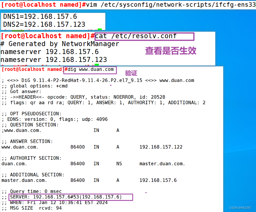
DNS解析和主从复制
一、DNS名称解析协议 二、DNS正向解析 三、DNS主从复制 主服务器 从服务器...
光猫(无限路由器)插入可移动硬盘搭建简易版的NAS
1.场景分析 最近查询到了许多有关NAS的资料,用来替代百度云盘等确实有很多优势,尤其是具有不限速(速度看自己配置)、私密性好、一次投入后续只需要电费即可等优势。鉴于手上没有可以用的资源-cpu、机箱、内存等,查询到…...

SpringIOC之support模块GenericGroovyApplicationContext
博主介绍:✌全网粉丝5W,全栈开发工程师,从事多年软件开发,在大厂呆过。持有软件中级、六级等证书。可提供微服务项目搭建与毕业项目实战,博主也曾写过优秀论文,查重率极低,在这方面有丰富的经验…...

Awesome 3D Gaussian Splatting Resources
GitHub - MrNeRF/awesome-3D-gaussian-splatting: Curated list of papers and resources focused on 3D Gaussian Splatting, intended to keep pace with the anticipated surge of research in the coming months. 3D Gaussian Splatting简明教程 - 知乎...
【镜像压缩】linux 上 SD/TF 卡镜像文件压缩到实际大小的简单方法(树莓派、nvidia jetson)
文章目录 1. 备份 SD/TF 卡为镜像文件2. 压缩镜像文件2.1. 多分区镜像文件的压缩(树莓派、普通 linux 系统等)2.2. 单分区镜像文件的压缩(Nvidia Jetson Nano 等) 3. 还原镜像文件到 SD/TF 卡4. 镜像还原后处理4.1. 镜像分区调整4…...
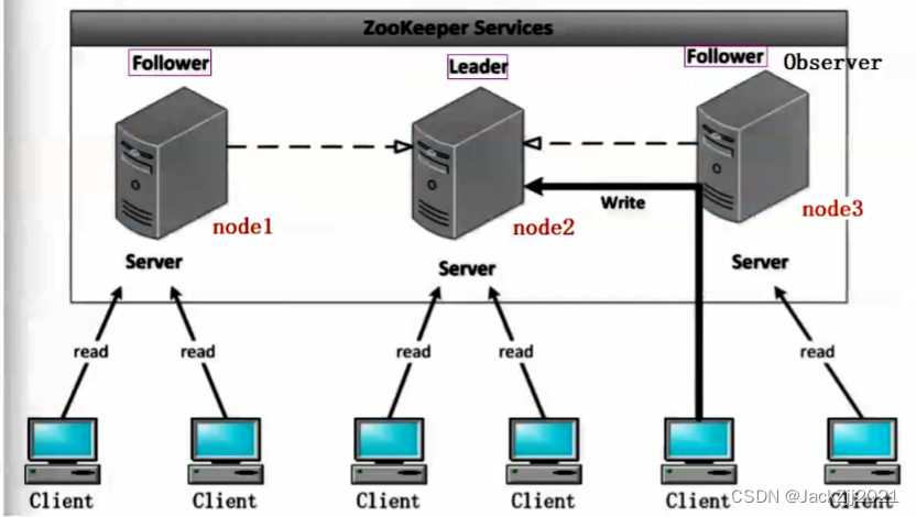
Zookeeper 和 naocs的区别
Nacos 和 ZooKeeper 都是服务发现和配置管理的工具,它们的主要区别如下:功能特性:Nacos 比 ZooKeeper 更加强大,Nacos 支持服务发现、动态配置、流量管理、服务治理、分布式事务等功能,而 ZooKeeper 主要用于分布式协调…...
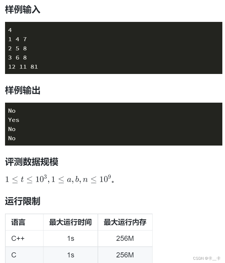
2-6基础算法-快速幂/倍增/构造
文章目录 一.快速幂二.倍增三.构造 一.快速幂 快速幂算法是一种高效计算幂ab的方法,特别是当b非常大时。它基于幂运算的性质,将幂运算分解成一系列的平方操作,以此减少乘法的次数。算法的核心在于将指数b表示为二进制形式,并利用…...

行业内参~移动广告行业大盘趋势-2023年12月
前言 2024年,移动广告的钱越来越难赚了。市场竞争激烈到前所未有的程度,小型企业和独立开发者在巨头的阴影下苦苦挣扎。随着广告成本的上升和点击率的下降,许多原本依赖广告收入的创业者和自由职业者开始感受到前所未有的压力。 dz…...

【笔记】书生·浦语大模型实战营——第四课(XTuner 大模型单卡低成本微调实战)
【参考:tutorial/xtuner/README.md at main InternLM/tutorial】 【参考:(4)XTuner 大模型单卡低成本微调实战_哔哩哔哩_bilibili-【OpenMMLab】】 总结 学到了 linux系统中 tmux 的使用 了解了 XTuner 大模型微调框架的使用 pth格式参数转Hugging …...

开源的Immich自建一个堪比 iCloud 的私有云相册和备份服务
源码地址 GitHub - immich-app/immich: Self-hosted photo and video backup solution directly from your mobile phone. 1.创建目录 mkdir /data/immich && cd /data/immich 2.下载docker-compose文件和.env文件 wget https://github.com/immich-app/immich/relea…...
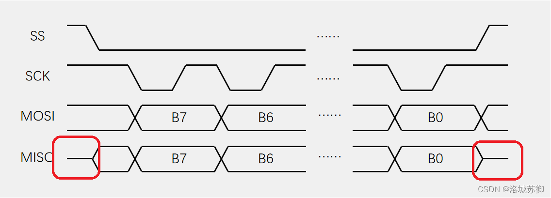
SPI通信讲解
了解SPI通信对于我们了解通信有非常重要的意义。 SPI(Serial Peripheral Interface)是由Motorola公司(摩托罗拉)开发的一种通用数据总线 四根通信线: SCK(Serial Clock):时钟线&a…...

本地一键部署grafana+prometheus
本地k8s集群内一键部署grafanaprometheus 说明: 此一键部署grafanaPrometheus已包含: victoria-metrics 存储prometheus-servergrafanaprometheus-kube-state-metricsprometheus-node-exporterblackbox-exporter grafana内已导入基础的dashboard【7个…...

NIO核心依赖多路复用小记
NIO允许一个线程同时处理多个连接,而不会因为一个连接的阻塞而导致其他连接被阻塞。核心是依赖操作系统的多路复用机制。 操作系统的多路复用机制 多路复用是一种操作系统的 I/O 处理机制,允许单个进程(或线程)同时监视多个输入…...

如何彻底卸载 Microsoft Edge?
关闭 Microsoft Edge 浏览器和所有正在运行的进程。 按下 Ctrl Shift Esc 键打开任务管理器。在任务管理器中,找到所有正在运行的 Microsoft Edge 进程。右键单击每个进程,然后选择“结束任务”。 导航至 Microsoft Edge 的安装目录。 默认情况下&…...

JavaScript-对象-笔记
1.字面量创建对象、对象的使用 对象就是一组 属性和方法的集合 属性: 特征 相当于变量 静态 是什么 方法: 行为 相当于函数 动态 干什么 创建对象 创建对象的第一种:使用字面量 {} 对象中的元素是键值对 使用逗号隔开 键:值 的形式 var 对象名…...

颠覆式Alienware设备控制:500KB轻量工具实现10倍性能提升与个性化体验
颠覆式Alienware设备控制:500KB轻量工具实现10倍性能提升与个性化体验 【免费下载链接】alienfx-tools Alienware systems lights, fans, and power control tools and apps 项目地址: https://gitcode.com/gh_mirrors/al/alienfx-tools 当你启动Alienware电…...

重塑暗黑2单机体验:d2s-editor 3大革新功能与技术解析
重塑暗黑2单机体验:d2s-editor 3大革新功能与技术解析 【免费下载链接】d2s-editor 项目地址: https://gitcode.com/gh_mirrors/d2/d2s-editor d2s-editor 是一款开源的暗黑2存档编辑工具,通过直观的图形界面实现角色属性调整、装备管理和高级合…...

Ardyno库:Dynamixel伺服电机的嵌入式底层通信框架
1. Ardyno库概述:面向Dynamixel伺服电机的嵌入式控制框架Ardyno是一个专为嵌入式平台设计的轻量级C/C库,用于精确、可靠地控制Robotis公司系列Dynamixel智能伺服电机(如AX-12A、MX-28、XL-320、XH430、XM430等)。其核心价值不在于…...

Thorium浏览器:重新定义现代网页浏览体验的高性能解决方案
Thorium浏览器:重新定义现代网页浏览体验的高性能解决方案 【免费下载链接】thorium Chromium fork named after radioactive element No. 90. Source code and Linux releases. Windows/MacOS/ARM builds served in different repos, links are towards the top of…...

MindSpore 环境配置完全指南
1 安装与初始化 # 全局安装 OpenSpec npm install -g fission-ai/openspeclatest # 在项目目录下初始化 cd /path/to/your-project openspec init 初始化时,OpenSpec 会提示你选择使用的 AI 工具(Claude Code、Cursor、Trae、Qoder 等)。 3 O…...

智能邮件中枢:OpenClaw+Qwen3.5-9B自动分类回复系统
智能邮件中枢:OpenClawQwen3.5-9B自动分类回复系统 1. 为什么需要自动化邮件处理 每天早晨打开邮箱,看到堆积如山的未读邮件时,那种窒息感我太熟悉了。作为外贸团队的独立开发者,我经常需要同时处理客户询盘、供应商报价、内部协…...

如何通过4个步骤让百度网盘下载速度提升30倍?
如何通过4个步骤让百度网盘下载速度提升30倍? 【免费下载链接】baidu-wangpan-parse 获取百度网盘分享文件的下载地址 项目地址: https://gitcode.com/gh_mirrors/ba/baidu-wangpan-parse 还在为百度网盘几十KB的下载速度而焦虑吗?百度网盘直链解…...

从毫安预警到安培计量:芯森电子FR系列传感器在储能安全与管理中的协同应用
摘要在储能系统(ESS)的安全架构中,电流传感器不仅是计量工具,更是系统的“免疫细胞”。随着储能系统向高压化、数字化演进,单一的电流检测方案已无法满足从“微小漏电预警”到“电池主回路控制”的全栈需求。本文基于芯…...

终极指南:如何用VideoSrt在5分钟内为视频自动生成字幕
终极指南:如何用VideoSrt在5分钟内为视频自动生成字幕 【免费下载链接】video-srt-windows 这是一个可以识别视频语音自动生成字幕SRT文件的开源 Windows-GUI 软件工具。 项目地址: https://gitcode.com/gh_mirrors/vi/video-srt-windows 还在为手动添加字幕…...

2026年毕业论文写作避坑:学术AI工具怎么选才靠谱?
每到开题季,后台总会收到相似的问题:现在AI这么强,写论文到底该用哪个?不少同学的教训是——随便找个通用聊天AI,输入题目“一键生成”几万字,结果查重不过、AI检测亮红灯、参考文献全是编的,导…...