深度学习之pytorch实现线性回归

pytorch用到的函数

torch.nn.Linearn()函数

torch.nn.Linear(in_features, # 输入的神经元个数out_features, # 输出神经元个数bias=True # 是否包含偏置)

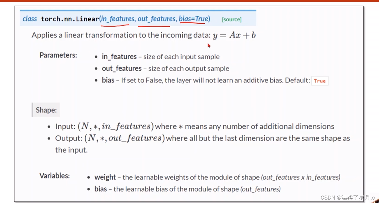
作用j进行线性变换
Linear(1, 1) : 表示一维输入，一维输出

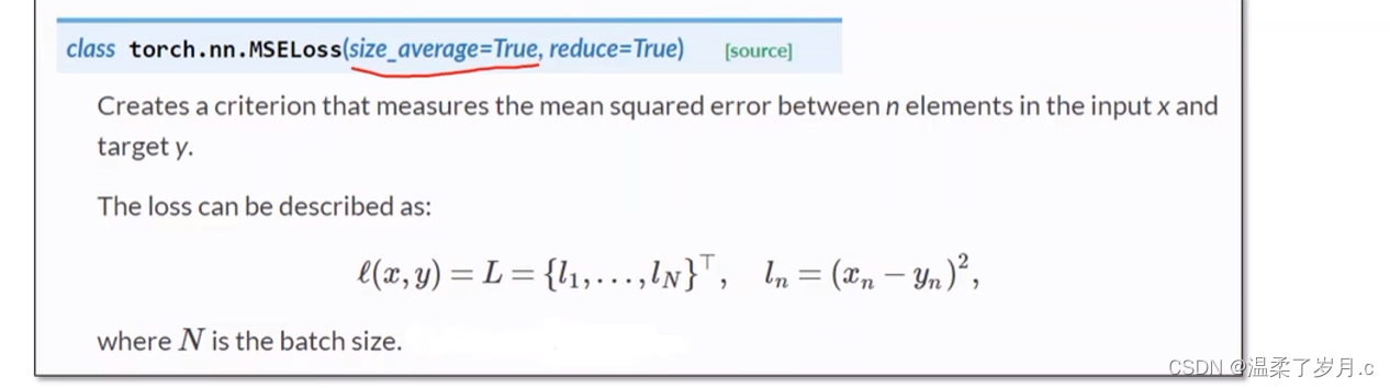
torch.nn.MSELoss()函数

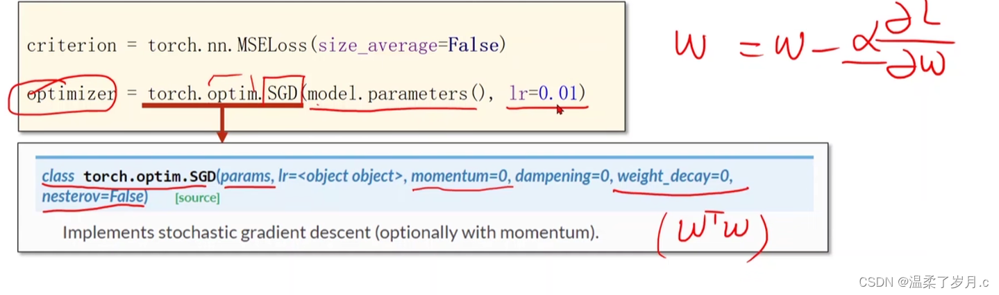
torch.optim.SGD()

优化器对象

代码实现

import torchx_data = torch.tensor([[1.0], [2.0], [3.0]])  # 将x_data设置为tensor类型数据
y_data = torch.tensor([[2.0], [4.0], [6.0]])class LinearModel(torch.nn.Module):def __init__(self):super(LinearModel, self).__init__()  # 继承父类self.linear = torch.nn.Linear(1, 1)# 用torch.nn.Linear来构造对象  (y = w * x + b)def forward(self, x):y_pred = self.linear(x) #调用之前的构造的对象(调用构造函数)，计算 y = w * x + breturn y_predmodel = LinearModel()criterion = torch.nn.MSELoss(size_average=False)  # 定义损失函数，不求平均损失(为False)#优化器对象
# #model.parameters()会扫描module中的所有成员，如果成员中有相应权重，那么都会将结果加到要训练的参数集合上
# #类似权重的更新
optimizer = torch.optim.SGD(model.parameters(), lr=0.01)  # 定义梯度优化器为随机梯度下降for epoch in range(10000):  # 训练过程y_pred = model(x_data)  # 向前传播，求y_predloss = criterion(y_pred, y_data)  # 根据y_pred和y_data求损失print(epoch, loss)# 记住在backward之前要先梯度归零optimizer.zero_grad()  # 将优化器数值清零loss.backward()  # 反向传播，计算梯度optimizer.step()  # 根据梯度更新参数#打印权重和b
print("w = ", model.linear.weight.item())
print("b = ", model.linear.bias.item())#检测模型
x_test = torch.tensor([4.0])
y_test = model(x_test)
print('y_pred = ', y_test.data)  # 测试

结果分析

9961 tensor(4.0927e-12, grad_fn=)
9962 tensor(4.0927e-12, grad_fn=)
9963 tensor(4.0927e-12, grad_fn=)
9964 tensor(4.0927e-12, grad_fn=)
9965 tensor(4.0927e-12, grad_fn=)
9966 tensor(4.0927e-12, grad_fn=)
9967 tensor(4.0927e-12, grad_fn=)
9968 tensor(4.0927e-12, grad_fn=)
9969 tensor(4.0927e-12, grad_fn=)
9970 tensor(4.0927e-12, grad_fn=)
9971 tensor(4.0927e-12, grad_fn=)
9972 tensor(4.0927e-12, grad_fn=)
9973 tensor(4.0927e-12, grad_fn=)
9974 tensor(4.0927e-12, grad_fn=)
9975 tensor(4.0927e-12, grad_fn=)
9976 tensor(4.0927e-12, grad_fn=)
9977 tensor(4.0927e-12, grad_fn=)
9978 tensor(4.0927e-12, grad_fn=)
9979 tensor(4.0927e-12, grad_fn=)
9980 tensor(4.0927e-12, grad_fn=)
9981 tensor(4.0927e-12, grad_fn=)
9982 tensor(4.0927e-12, grad_fn=)
9983 tensor(4.0927e-12, grad_fn=)
9984 tensor(4.0927e-12, grad_fn=)
9985 tensor(4.0927e-12, grad_fn=)
9986 tensor(4.0927e-12, grad_fn=)
9987 tensor(4.0927e-12, grad_fn=)
9988 tensor(4.0927e-12, grad_fn=)
9989 tensor(4.0927e-12, grad_fn=)
9990 tensor(4.0927e-12, grad_fn=)
9991 tensor(4.0927e-12, grad_fn=)
9992 tensor(4.0927e-12, grad_fn=)
9993 tensor(4.0927e-12, grad_fn=)
9994 tensor(4.0927e-12, grad_fn=)
9995 tensor(4.0927e-12, grad_fn=)
9996 tensor(4.0927e-12, grad_fn=)
9997 tensor(4.0927e-12, grad_fn=)
9998 tensor(4.0927e-12, grad_fn=)
9999 tensor(4.0927e-12, grad_fn=)

w = 1.9999985694885254
b = 2.979139480885351e-06
y_pred = tensor([8.0000])

因为轮数过多，这里展示后面几轮
模型的准确性，跟轮数的多少有关系 ，如果轮数为100，最后测试结果的y_pred肯定不为8.00，这里轮数为10000,预测结果跟实际结果基本一样

这里是轮数为100，结果是 7点多，有一定误差
0 tensor(101.4680, grad_fn=)
1 tensor(45.8508, grad_fn=)
2 tensor(21.0819, grad_fn=)
3 tensor(10.0458, grad_fn=)
4 tensor(5.1234, grad_fn=)
5 tensor(2.9227, grad_fn=)
6 tensor(1.9338, grad_fn=)
7 tensor(1.4844, grad_fn=)
8 tensor(1.2754, grad_fn=)
9 tensor(1.1736, grad_fn=)
10 tensor(1.1195, grad_fn=)
11 tensor(1.0869, grad_fn=)
12 tensor(1.0639, grad_fn=)
13 tensor(1.0453, grad_fn=)
14 tensor(1.0288, grad_fn=)
15 tensor(1.0134, grad_fn=)
16 tensor(0.9985, grad_fn=)
17 tensor(0.9841, grad_fn=)
18 tensor(0.9699, grad_fn=)
19 tensor(0.9559, grad_fn=)
20 tensor(0.9421, grad_fn=)
21 tensor(0.9286, grad_fn=)
22 tensor(0.9153, grad_fn=)
23 tensor(0.9021, grad_fn=)
24 tensor(0.8891, grad_fn=)
25 tensor(0.8764, grad_fn=)
26 tensor(0.8638, grad_fn=)
27 tensor(0.8513, grad_fn=)
28 tensor(0.8391, grad_fn=)
29 tensor(0.8271, grad_fn=)
30 tensor(0.8152, grad_fn=)
31 tensor(0.8034, grad_fn=)
32 tensor(0.7919, grad_fn=)
33 tensor(0.7805, grad_fn=)
34 tensor(0.7693, grad_fn=)
35 tensor(0.7582, grad_fn=)
36 tensor(0.7474, grad_fn=)
37 tensor(0.7366, grad_fn=)
38 tensor(0.7260, grad_fn=)
39 tensor(0.7156, grad_fn=)
40 tensor(0.7053, grad_fn=)
41 tensor(0.6952, grad_fn=)
42 tensor(0.6852, grad_fn=)
43 tensor(0.6753, grad_fn=)
44 tensor(0.6656, grad_fn=)
45 tensor(0.6561, grad_fn=)
46 tensor(0.6466, grad_fn=)
47 tensor(0.6373, grad_fn=)
48 tensor(0.6282, grad_fn=)
49 tensor(0.6192, grad_fn=)
50 tensor(0.6103, grad_fn=)
51 tensor(0.6015, grad_fn=)
52 tensor(0.5928, grad_fn=)
53 tensor(0.5843, grad_fn=)
54 tensor(0.5759, grad_fn=)
55 tensor(0.5676, grad_fn=)
56 tensor(0.5595, grad_fn=)
57 tensor(0.5514, grad_fn=)
58 tensor(0.5435, grad_fn=)
59 tensor(0.5357, grad_fn=)
60 tensor(0.5280, grad_fn=)
61 tensor(0.5204, grad_fn=)
62 tensor(0.5129, grad_fn=)
63 tensor(0.5056, grad_fn=)
64 tensor(0.4983, grad_fn=)
65 tensor(0.4911, grad_fn=)
66 tensor(0.4841, grad_fn=)
67 tensor(0.4771, grad_fn=)
68 tensor(0.4703, grad_fn=)
69 tensor(0.4635, grad_fn=)
70 tensor(0.4569, grad_fn=)
71 tensor(0.4503, grad_fn=)
72 tensor(0.4438, grad_fn=)
73 tensor(0.4374, grad_fn=)
74 tensor(0.4311, grad_fn=)
75 tensor(0.4250, grad_fn=)
76 tensor(0.4188, grad_fn=)
77 tensor(0.4128, grad_fn=)
78 tensor(0.4069, grad_fn=)
79 tensor(0.4010, grad_fn=)
80 tensor(0.3953, grad_fn=)
81 tensor(0.3896, grad_fn=)
82 tensor(0.3840, grad_fn=)
83 tensor(0.3785, grad_fn=)
84 tensor(0.3730, grad_fn=)
85 tensor(0.3677, grad_fn=)
86 tensor(0.3624, grad_fn=)
87 tensor(0.3572, grad_fn=)
88 tensor(0.3521, grad_fn=)
89 tensor(0.3470, grad_fn=)
90 tensor(0.3420, grad_fn=)
91 tensor(0.3371, grad_fn=)
92 tensor(0.3322, grad_fn=)
93 tensor(0.3275, grad_fn=)
94 tensor(0.3228, grad_fn=)
95 tensor(0.3181, grad_fn=)
96 tensor(0.3136, grad_fn=)
97 tensor(0.3091, grad_fn=)
98 tensor(0.3046, grad_fn=)
99 tensor(0.3002, grad_fn=)
w = 1.6352288722991943
b = 0.8292105793952942
y_pred = tensor([7.3701])

Process finished with exit code 0