【计算机视觉】Gaussian Splatting源码解读补充(二)
- 第一部分
本文是对学习笔记之——3D Gaussian Splatting源码解读的补充,并订正了一些错误。
目录
- 三、相机相关
- `scene/cameras.py`:`class Camera`
- 四、前向传播(渲染):`submodules/diff-gaussian-rasterization/cuda_rasterizer/forward.cu`
- 预备知识:CUDA编程基础
- `def render(viewpoint_camera, pc : GaussianModel, pipe, bg_color : torch.Tensor, scaling_modifier = 1.0, override_color = None)`
- CUDA文件`rasterizer_impl.cu`: `submodules/diff-gaussian-rasterization/cuda_rasterizer`
- 1. 引用头文件
- (1) Cooperative Groups
- (2) CUB
- (3) GLM
- 2. `getHigherMsb`
- 3. `checkFrustum`和`markVisible`
- 4. 几个`fromChunk`
- 5. 为排序做准备:`duplicateWithKeys`
- 6. 排序之后的处理:`identifyTileRanges`
- 7. 重头戏:前向传播`forward`
- CUDA文件`forward.cu`: `submodules/diff-gaussian-rasterization/cuda_rasterizer`
- 1. `computeColorFromSH`
- 2. `computeCov2D`
- 3. `computeCov3D`
- 4. `preprocessCUDA`
- 5. `render`和`renderCUDA`
三、相机相关
scene/cameras.py:class Camera
class Camera(nn.Module):def __init__(self, colmap_id, R, T, FoVx, FoVy, image, gt_alpha_mask,image_name, uid,trans=np.array([0.0, 0.0, 0.0]), scale=1.0, data_device = "cuda"):super(Camera, self).__init__()self.uid = uidself.colmap_id = colmap_idself.R = R # 旋转矩阵self.T = T # 平移向量self.FoVx = FoVx # x方向视场角self.FoVy = FoVy # y方向视场角self.image_name = image_nametry:self.data_device = torch.device(data_device)except Exception as e:print(e)print(f"[Warning] Custom device {data_device} failed, fallback to default cuda device" )self.data_device = torch.device("cuda")self.original_image = image.clamp(0.0, 1.0).to(self.data_device) # 原始图像self.image_width = self.original_image.shape[2] # 图像宽度self.image_height = self.original_image.shape[1] # 图像高度if gt_alpha_mask is not None:self.original_image *= gt_alpha_mask.to(self.data_device)else:self.original_image *= torch.ones((1, self.image_height, self.image_width), device=self.data_device)# 距离相机平面znear和zfar之间且在视锥内的物体才会被渲染self.zfar = 100.0 # 最远能看到多远self.znear = 0.01 # 最近能看到多近self.trans = trans # 相机中心的平移self.scale = scale # 相机中心坐标的缩放self.world_view_transform = torch.tensor(getWorld2View2(R, T, trans, scale)).transpose(0, 1).cuda() # 世界到相机坐标系的变换矩阵,4×4self.projection_matrix = getProjectionMatrix(znear=self.znear, zfar=self.zfar, fovX=self.FoVx, fovY=self.FoVy).transpose(0,1).cuda() # 投影矩阵self.full_proj_transform = (self.world_view_transform.unsqueeze(0).bmm(self.projection_matrix.unsqueeze(0))).squeeze(0) # 从世界坐标系到图像的变换矩阵self.camera_center = self.world_view_transform.inverse()[3, :3] # 相机在世界坐标系下的坐标
其中出现的辅助函数:
# utils/graphic_utils.py
def getWorld2View2(R, t, translate=np.array([.0, .0, .0]), scale=1.0):Rt = np.zeros((4, 4)) # 按理来说是世界到相机的变换矩阵,但没有加平移和缩放Rt[:3, :3] = R.transpose()Rt[:3, 3] = tRt[3, 3] = 1.0C2W = np.linalg.inv(Rt) # 相机到世界的变换矩阵cam_center = C2W[:3, 3] # 相机中心在世界中的坐标,即C2W矩阵第四列的三维平移向量cam_center = (cam_center + translate) * scale # 相机中心坐标需要平移和缩放处理C2W[:3, 3] = cam_center # 重新填入C2W矩阵Rt = np.linalg.inv(C2W) # 再取逆获得W2C矩阵return np.float32(Rt)
四、前向传播(渲染):submodules/diff-gaussian-rasterization/cuda_rasterizer/forward.cu
预备知识:CUDA编程基础
这部分的参考资料:
[1] CUDA Tutorial
[2] An Even Easier Introduction to CUDA
[3] Introduction to CUDA Programming
CUDA是一个为支持CUDA的GPU提供的平台和编程模型。该平台使GPU能够进行通用计算。CUDA提供了C/C++语言扩展和API,以便用户利用GPU进行高效计算。一般称CPU为host,GPU为device。
CUDA C++语言中有一个加在函数前面的关键字__global__,用于表明该函数是运行在GPU上的,并且可以被CPU调用。这种函数称为kernel。
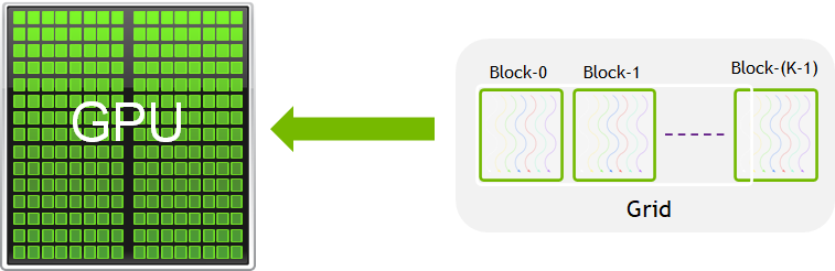
当我们调用kernel的时候,需要在函数名和括号之间加上<<<M, T>>>,其中M是block的个数,T是每个block中线程的个数。这些线程都是并行执行的,每个线程中都在执行该函数。
根据参考资料[3],GPU在同一时刻运行一个kernel(也就是一组任务),kernel运行在grid上,每个grid由多个block组成(他们是独立的ALU组),每个block有多个线程。
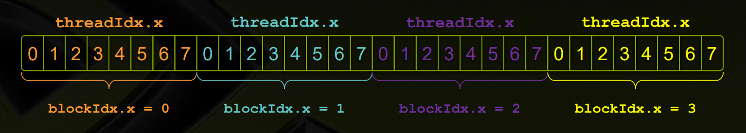
同一block中的线程一般合作完成任务,它们可以共享内存(这部分内存速度极快,用__shared__关键字声明)。每个线程“知道”它在哪个block(通过访问内置变量blockIdx.x)和它是第几个线程(通过访问变量threadIdx.x),以及每个block有多少个线程(blockDim.x),从而确定它应该完成什么任务。实际上线程和block的索引是三维的,这里只举了一个一维的例子。
注意GPU和CPU的内存是隔离的,想要操作显存或者在显存和CPU内存之间进行交流必须显示的声明这些操作。指针也是不一样的,有可能虽然都是int*,但表示的含义却不同:device指针指向显存,host指针指向CPU内存。CUDA提供了操作内存的内置函数:cudaMalloc、cudaFree、cudaMemcpy等,它们分别类似于C函数malloc、free和memcpy。
关于同步方面,内置函数 __syncthreads()可以同步一个block中的所有线程。在CPU中调用内置函数cudaDeviceSynchronize()可以可以阻塞CPU,直到所有先前发出的CUDA调用都完成为止。
另外还有__host__关键字和__device__关键字,前者表示该函数只编译成CPU版本(这是默认状态),后者表示只编译成GPU版本。二者同时使用表示编译CPU和GPU两个版本。从CPU调用__device__函数和从GPU调用__host__函数都会报错。
以下是一个CUDA并行计算向量加法的示例:
#include <stdio.h>int a[10] = {0, 1, 2, 3, 4, 5, 6, 7, 8, 9};
int b[10] = {0, 10, 20, 30, 40, 50, 60, 70, 80, 90};
int c[10];__global__ void vec_add(int* A, int* B, int* C)
{int i = blockIdx.x * blockDim.x + threadIdx.x;C[i] = A[i] + B[i];
}int main()
{int* gpua, *gpub, *gpuc;int sz = 10 * sizeof(int);cudaMalloc((void**)&gpua, sz); // 在GPU中分配内存cudaMalloc((void**)&gpub, sz);cudaMalloc((void**)&gpuc, sz);cudaMemcpy(gpua, a, sz, cudaMemcpyHostToDevice); // 拷贝CPU中的数组到GPUcudaMemcpy(gpub, b, sz, cudaMemcpyHostToDevice);vec_add<<<2, 5>>>(gpua, gpub, gpuc); // 调用kernelcudaDeviceSynchronize(); // 等GPU执行完(这里其实不是很有必要)cudaMemcpy(c, gpuc, sz, cudaMemcpyDeviceToHost); // 把GPU的计算结果拷贝到CPUfor(int i = 0; i < 10; i++){printf("%d\n", c[i]); // 输出结果,结果为0、11、22、……、99}return 0;
}
有了这些预备知识之后,我们就可以开始看代码了。在看CUDA代码之前,我们先看看gaussian_renderer/__init__.py中的render函数。
def render(viewpoint_camera, pc : GaussianModel, pipe, bg_color : torch.Tensor, scaling_modifier = 1.0, override_color = None)
def render(viewpoint_camera, pc : GaussianModel, pipe, bg_color : torch.Tensor, scaling_modifier = 1.0, override_color = None):'''viewpoint_camera: scene.cameras.Camera类的实例pipe: 流水线,规定了要干什么'''# Create zero tensor. We will use it to make pytorch return gradients of the 2D (screen-space) meansscreenspace_points = torch.zeros_like(pc.get_xyz, dtype=pc.get_xyz.dtype, requires_grad=True, device="cuda") + 0try:screenspace_points.retain_grad() # 让screenspace_points在反向传播时接受梯度except:pass# Set up rasterization configurationtanfovx = math.tan(viewpoint_camera.FoVx * 0.5)tanfovy = math.tan(viewpoint_camera.FoVy * 0.5)raster_settings = GaussianRasterizationSettings(image_height=int(viewpoint_camera.image_height),image_width=int(viewpoint_camera.image_width),tanfovx=tanfovx,tanfovy=tanfovy,bg=bg_color, # 背景颜色scale_modifier=scaling_modifier,viewmatrix=viewpoint_camera.world_view_transform, # W2C矩阵projmatrix=viewpoint_camera.full_proj_transform, # 世界到图像的投影矩阵sh_degree=pc.active_sh_degree, # 目前的球谐阶数campos=viewpoint_camera.camera_center, # CAMera center POSition,相机中心文职prefiltered=False,debug=pipe.debug)rasterizer = GaussianRasterizer(raster_settings=raster_settings)means3D = pc.get_xyzmeans2D = screenspace_points # 疑似各个Gaussian的中心投影到在图像中的坐标opacity = pc.get_opacity # 不透明度# If precomputed 3d covariance is provided, use it. If not, then it will be computed from# scaling / rotation by the rasterizer.scales = Nonerotations = Nonecov3D_precomp = Noneif pipe.compute_cov3D_python:cov3D_precomp = pc.get_covariance(scaling_modifier)else:scales = pc.get_scalingrotations = pc.get_rotation# If precomputed colors are provided, use them. Otherwise, if it is desired to precompute colors# from SHs in Python, do it. If not, then SH -> RGB conversion will be done by rasterizer.shs = Nonecolors_precomp = Noneif override_color is None:if pipe.convert_SHs_python:shs_view = pc.get_features.transpose(1, 2).view(-1, 3, (pc.max_sh_degree+1)**2)dir_pp = (pc.get_xyz - viewpoint_camera.camera_center.repeat(pc.get_features.shape[0], 1))dir_pp_normalized = dir_pp/dir_pp.norm(dim=1, keepdim=True)# 找到高斯中心到相机的光线在单位球体上的坐标sh2rgb = eval_sh(pc.active_sh_degree, shs_view, dir_pp_normalized)# 球谐的傅里叶系数转成RGB颜色colors_precomp = torch.clamp_min(sh2rgb + 0.5, 0.0)else:shs = pc.get_featureselse:colors_precomp = override_color# Rasterize visible Gaussians to image, obtain their radii (on screen). rendered_image, radii = rasterizer(means3D = means3D,means2D = means2D,shs = shs,colors_precomp = colors_precomp,opacities = opacity,scales = scales,rotations = rotations,cov3D_precomp = cov3D_precomp)# Those Gaussians that were frustum culled or had a radius of 0 were not visible.# They will be excluded from value updates used in the splitting criteria.return {"render": rendered_image,"viewspace_points": screenspace_points,"visibility_filter" : radii > 0,"radii": radii}
CUDA文件rasterizer_impl.cu: submodules/diff-gaussian-rasterization/cuda_rasterizer
1. 引用头文件
#include "rasterizer_impl.h"
#include <iostream>
#include <fstream>
#include <algorithm>
#include <numeric>
#include <cuda.h>
#include "cuda_runtime.h"
#include "device_launch_parameters.h"
#include <cub/cub.cuh> // CUDA的CUB库
#include <cub/device/device_radix_sort.cuh>
#define GLM_FORCE_CUDA
#include <glm/glm.hpp> // GLM (OpenGL Mathematics)库#include <cooperative_groups.h> // CUDA 9引入的Cooperative Groups库
#include <cooperative_groups/reduce.h>
namespace cg = cooperative_groups;#include "auxiliary.h"
#include "forward.h"
#include "backward.h"
有一些库需要我们讲解一下。
(1) Cooperative Groups
参考资料:
- Cooperative Groups: Flexible CUDA Thread Programming
- 这个库的官方文档
我们直到 __syncthreads()函数提供了在一个block内同步各线程的方法,但有时要同步block内的一部分线程或者多个block的线程,这时候就需要Cooperative Groups库了。这个库定义了划分和同步一组线程的方法。
在Gaussian Splatting的所有CUDA代码中,这个库仅以两种方式被调用:
🥕(a)
auto idx = cg::this_grid().thread_rank();
cg::this_grid()返回一个cg::grid_group实例,表示当前线程所处的grid。他有一个方法thread_rank()返回当前线程在该grid中排第几。
🥕(b)
auto block = cg::this_thread_block();
cg::this_thread_block返回一个cg::thread_block实例。代码中用到的成员函数有:
block.sync():同步该block中的所有线程(等价于__syncthreads())。block.thread_rank():返回非负整数,表示当前线程在该block中排第几。block.group_index():返回一个cg::dim3实例,表示该block在grid中的三维索引。block.thread_index():返回一个cg::dim3实例,表示当前线程在block中的三维索引。
(2) CUB
参考资料:CUB API
CUB provides layered algorithms that correspond to the thread/warp/block/device hierarchy of threads in CUDA. There are distinct algorithms for each layer and higher-level layers build on top of those below.
换言之,CUB就是针对不同的计算等级:线程、wap、block、device等设计了并行算法。例如,reduce函数有四个版本:ThreadReduce、WarpReduce、BlockReduce、DeviceReduce。
diff-gaussian-rasterization模块调用了CUB库的两个函数:
⭐️ (a) cub::DeviceScan::InclusiveSum
这个函数是算前缀和的。所谓"Inclusive"就是第 i i i个数被计入第 i i i个和中。函数定义如下:
template<typename InputIteratorT, typename OutputIteratorT>
static inline cudaError_t InclusiveSum(void *d_temp_storage, // 额外需要的临时显存空间size_t &temp_storage_bytes, // 临时显存空间的大小InputIteratorT d_in, // 输入指针OutputIteratorT d_out, // 输出指针int num_items, // 元素个数cudaStream_t stream = 0)
⭐️ (b) cub::DeviceRadixSort::SortPairs:device级别的并行基数排序
该函数根据key将(key, value)对进行升序排序。这是一种稳定排序。
函数定义如下:
template<typename KeyT, typename ValueT, typename NumItemsT>
static inline cudaError_t SortPairs(void *d_temp_storage, // 排序时用到的临时显存空间size_t &temp_storage_bytes, // 临时显存空间的大小const KeyT *d_keys_in,         KeyT *d_keys_out, // key的输入和输出指针const ValueT *d_values_in,     ValueT *d_values_out, // value的输入和输出指针NumItemsT num_items, // 对多少个条目进行排序int begin_bit = 0, // 低位int end_bit = sizeof(KeyT) * 8, // 高位cudaStream_t stream = 0)// 按照[begin_bit, end_bit)内的位进行排序
示例代码:
#include <stdio.h>
#include <cub/cub.cuh>
// or equivalently <cub/device/device_radix_sort.cuh>int main()
{// Declare, allocate, and initialize device-accessible pointers// for sorting dataint  num_items = 7;int  keys_in[7] = {8, 6, 7, 5, 3, 0, 9};int* d_keys_in, *d_keys_out;int  values_in[7] = {0, 1, 2, 3, 4, 5, 6};int* d_values_in, *d_values_out;int keys_out[7], values_out[7];// 下面把数据搬到显存中int sz = 7 * sizeof(int);cudaMalloc((void**)&d_values_in, sz);cudaMalloc((void**)&d_values_out, sz);cudaMalloc((void**)&d_keys_in, sz);cudaMalloc((void**)&d_keys_out, sz);cudaMemcpy(d_keys_in, keys_in, sz, cudaMemcpyHostToDevice);cudaMemcpy(d_values_in, values_in, sz, cudaMemcpyHostToDevice);// Determine temporary device storage requirementsvoid     *d_temp_storage = NULL;size_t   temp_storage_bytes = 0;cub::DeviceRadixSort::SortPairs(d_temp_storage, temp_storage_bytes,d_keys_in, d_keys_out, d_values_in, d_values_out, num_items);// Allocate temporary storagecudaMalloc(&d_temp_storage, temp_storage_bytes);// Run sorting operationcub::DeviceRadixSort::SortPairs(d_temp_storage, temp_storage_bytes,d_keys_in, d_keys_out, d_values_in, d_values_out, num_items);// 结果:// d_keys_out            <-- [0, 3, 5, 6, 7, 8, 9]// d_values_out          <-- [5, 4, 3, 1, 2, 0, 6]// 把算好的数据搬回来cudaMemcpy(keys_out, d_keys_out, sz, cudaMemcpyDeviceToHost);cudaMemcpy(values_out, d_values_out, sz, cudaMemcpyDeviceToHost);puts("keys");for(int i = 0; i < 7; i++){printf("%d ", keys_out[i]);}puts("\nvalues");for(int i = 0; i < 7; i++){printf("%d ", values_out[i]);}cudaFree(d_keys_in);cudaFree(d_keys_out);cudaFree(d_values_in);cudaFree(d_values_out);return 0;
}
(3) GLM
参考资料:GLM的Github页面
GLM意为“OpenGL Mathematics”,是一个专为图形学设计的只有头文件的C++数学库。
Gaussian Splatting的代码中用到了glm::vec3(三维向量), glm::vec4(四维向量), glm::mat3(3×3矩阵)和glm::dot(向量点积)。
2. getHigherMsb
// Helper function to find the next-highest bit of the MSB
// on the CPU.
uint32_t getHigherMsb(uint32_t n)
{uint32_t msb = sizeof(n) * 4;uint32_t step = msb;while (step > 1){step /= 2;if (n >> msb)msb += step;elsemsb -= step;}if (n >> msb)msb++;return msb;
}
这个函数似乎是用二分法检测n表示成二进制数除去前导零有几位(n=0时返回1)。我写了一个测试程序推测它的功能:
#include <iostream>
uint32_t getHigherMsb(uint32_t n);int main()
{uint32_t n[] = {0b0, 0b1, 0b10, 0b11, 0b111, 0b10101, 0b1110001};for(int i = 0; i < sizeof(n) / sizeof(uint32_t); i++)std::cout << getHigherMsb(n[i]) << ", ";// 结果:1, 1, 2, 2, 3, 5, 7,
}
该函数只被调用过一次(在CudaRasterizer::Rasterizer::forward函数中),我们随后再推断它的具体含义。
3. checkFrustum和markVisible
根据函数命名和上下文推断,这两个函数的作用是检查一些Gaussians是否在一个给定相机的视锥内,从而确定它能不能被该相机看见。
// Wrapper method to call auxiliary coarse frustum containment test.
// Mark all Gaussians that pass it.
__global__ void checkFrustum(int P, // 需要检查的点的个数const float* orig_points, // 需要检查的点的世界坐标const float* viewmatrix, // W2C矩阵const float* projmatrix, // 投影矩阵bool* present) // 返回值,表示能不能被看见
{auto idx = cg::this_grid().thread_rank();if (idx >= P)return;float3 p_view;present[idx] = in_frustum(idx, orig_points, viewmatrix, projmatrix, false, p_view);
}// Mark Gaussians as visible/invisible, based on view frustum testing
void CudaRasterizer::Rasterizer::markVisible(int P,float* means3D, // Gaussians的中心点坐标float* viewmatrix,float* projmatrix,bool* present)
{checkFrustum << <(P + 255) / 256, 256 >> > (P,means3D,viewmatrix, projmatrix,present);
}
4. 几个fromChunk
这些函数的作用是从以char数组形式存储的二进制块中读取GeometryState、ImageState、BinningState等类的信息。
CudaRasterizer::GeometryState CudaRasterizer::GeometryState::fromChunk(char*& chunk, size_t P)
{GeometryState geom;obtain(chunk, geom.depths, P, 128);obtain(chunk, geom.clamped, P * 3, 128);obtain(chunk, geom.internal_radii, P, 128);obtain(chunk, geom.means2D, P, 128);obtain(chunk, geom.cov3D, P * 6, 128);obtain(chunk, geom.conic_opacity, P, 128);obtain(chunk, geom.rgb, P * 3, 128);obtain(chunk, geom.tiles_touched, P, 128);cub::DeviceScan::InclusiveSum(nullptr, geom.scan_size, geom.tiles_touched, geom.tiles_touched, P);obtain(chunk, geom.scanning_space, geom.scan_size, 128);obtain(chunk, geom.point_offsets, P, 128);return geom;
}CudaRasterizer::ImageState CudaRasterizer::ImageState::fromChunk(char*& chunk, size_t N)
{ImageState img;obtain(chunk, img.accum_alpha, N, 128);obtain(chunk, img.n_contrib, N, 128);obtain(chunk, img.ranges, N, 128);return img;
}CudaRasterizer::BinningState CudaRasterizer::BinningState::fromChunk(char*& chunk, size_t P)
{BinningState binning;obtain(chunk, binning.point_list, P, 128);obtain(chunk, binning.point_list_unsorted, P, 128);obtain(chunk, binning.point_list_keys, P, 128);obtain(chunk, binning.point_list_keys_unsorted, P, 128);cub::DeviceRadixSort::SortPairs(nullptr, binning.sorting_size,binning.point_list_keys_unsorted, binning.point_list_keys,binning.point_list_unsorted, binning.point_list, P);obtain(chunk, binning.list_sorting_space, binning.sorting_size, 128);return binning;
}
5. 为排序做准备:duplicateWithKeys
// Generates one key/value pair for all Gaussian / tile overlaps.
// Run once per Gaussian (1:N mapping).
__global__ void duplicateWithKeys(int P,const float2* points_xy,const float* depths,const uint32_t* offsets,uint64_t* gaussian_keys_unsorted,uint32_t* gaussian_values_unsorted,int* radii,dim3 grid)
{auto idx = cg::this_grid().thread_rank(); // 线程索引,该显线程处理第idx个Gaussianif (idx >= P)return;// Generate no key/value pair for invisible Gaussiansif (radii[idx] > 0){// Find this Gaussian's offset in buffer for writing keys/values.uint32_t off = (idx == 0) ? 0 : offsets[idx - 1];uint2 rect_min, rect_max;getRect(points_xy[idx], radii[idx], rect_min, rect_max, grid);// 因为要给Gaussian覆盖的每个tile生成一个(key, value)对,// 所以先获取它占了哪些tile// For each tile that the bounding rect overlaps, emit a // key/value pair. The key is |  tile ID  |      depth      |,// and the value is the ID of the Gaussian. Sorting the values // with this key yields Gaussian IDs in a list, such that they// are first sorted by tile and then by depth. for (int y = rect_min.y; y < rect_max.y; y++){for (int x = rect_min.x; x < rect_max.x; x++){uint64_t key = y * grid.x + x; // tile的IDkey <<= 32; // 放在高位key |= *((uint32_t*)&depths[idx]); // 低位是深度gaussian_keys_unsorted[off] = key;gaussian_values_unsorted[off] = idx;off++; // 数组中的偏移量}}}
}
6. 排序之后的处理:identifyTileRanges
// Check keys to see if it is at the start/end of one tile's range in
// the full sorted list. If yes, write start/end of this tile.
// Run once per instanced (duplicated) Gaussian ID.
__global__ void identifyTileRanges(int L, // 排序列表中的元素个数uint64_t* point_list_keys, // 排过序的keysuint2* ranges)// ranges[tile_id].x和y表示第tile_id个tile在排过序的列表中的起始和终止地址
{auto idx = cg::this_grid().thread_rank();if (idx >= L)return;// Read tile ID from key. Update start/end of tile range if at limit.uint64_t key = point_list_keys[idx];uint32_t currtile = key >> 32; // 当前tileif (idx == 0)ranges[currtile].x = 0; // 边界条件:tile 0的起始位置else{uint32_t prevtile = point_list_keys[idx - 1] >> 32;if (currtile != prevtile)// 上一个元素和我处于不同的tile,// 那我是上一个tile的终止位置和我所在tile的起始位置{ranges[prevtile].y = idx;ranges[currtile].x = idx;}}if (idx == L - 1)ranges[currtile].y = L; // 边界条件:最后一个tile的终止位置
}
7. 重头戏:前向传播forward
原文第6节(FAST DIFFERENTIABLE RASTERIZER FOR GAUSSIANS):
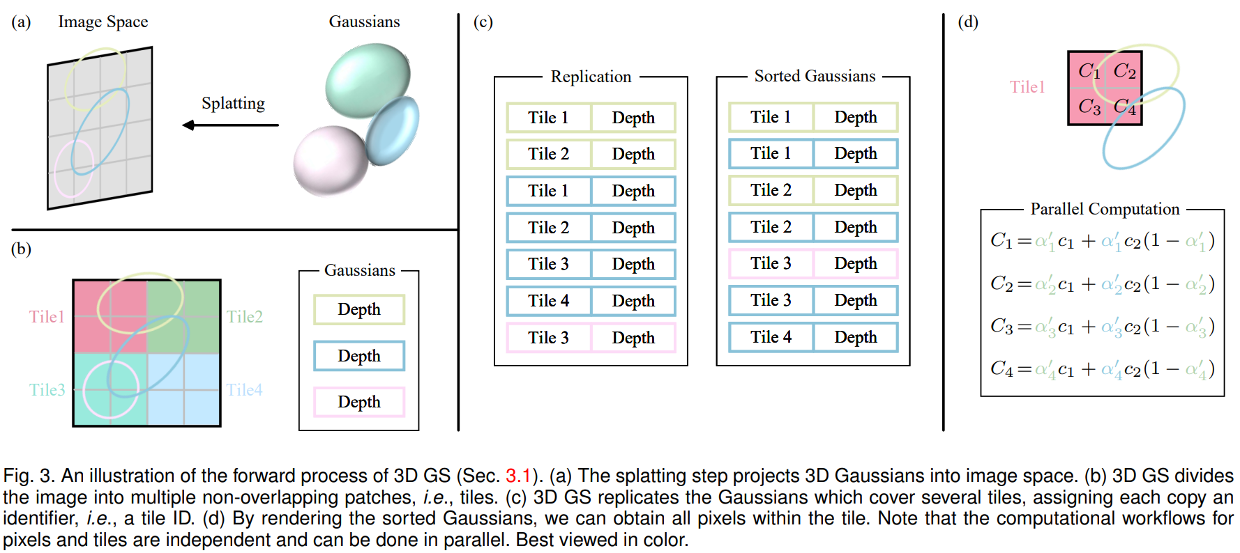
Our method starts by splitting the screen into 16×16 tiles, and then proceeds to cull 3D Gaussians against the view frustum and each tile. Specifically, we only keep Gaussians with a 99% confidence interval intersecting the view frustum. Additionally, we use a guard band to trivially reject Gaussians at extreme positions (i.e., those with means close to the near plane and far outside the view frustum), since computing their projected 2D covariance would be unstable. We then instantiate each Gaussian according to the number of tiles they overlap and assign each instance a key that combines view space depth and tile ID. We then sort Gaussians based on these keys using a single fast GPU Radix sort [Merrill and Grimshaw 2010]. Note that there is no additional per-pixel ordering of points, and blending is performed based on this initial sorting. As a consequence, our 𝛼-blending can be approximate in some configurations. However, these approximations become negligible as splats approach the size of individual pixels. We found that this choice greatly enhances training and rendering performance without producing visible artifacts in converged scenes.
After sorting Gaussians, we produce a list for each tile by identifying the first and last depth-sorted entry that splats to a given tile. For rasterization, we launch one thread block for each tile. Each block first collaboratively loads packets of Gaussians into shared memory and then, for a given pixel, accumulates color and 𝛼 values by traversing the lists front-to-back, thus maximizing the gain in parallelism both for data loading/sharing and processing. When we reach a target saturation of 𝛼 in a pixel, the corresponding thread stops. At regular intervals, threads in a tile are queried and the processing of the entire tile terminates when all pixels have saturated (i.e., 𝛼 goes to 1). Details of sorting and a high-level overview of the overall rasterization approach are given in Appendix C.
During rasterization, the saturation of 𝛼 is the only stopping criterion. In contrast to previous work, we do not limit the number of blended primitives that receive gradient updates. We enforce this property to allow our approach to handle scenes with an arbitrary, varying depth complexity and accurately learn them, without having to resort to scene-specific hyperparameter tuning.
附录C中的伪代码如下:
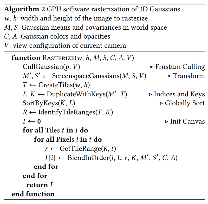
前向传播过程可以用该图片概括(出处:A Survey on 3D Gaussian Splatting):
// Forward rendering procedure for differentiable rasterization
// of Gaussians.
int CudaRasterizer::Rasterizer::forward(std::function<char* (size_t)> geometryBuffer,std::function<char* (size_t)> binningBuffer,std::function<char* (size_t)> imageBuffer,/*上面的三个参数是用于分配缓冲区的函数,在submodules/diff-gaussian-rasterization/rasterize_points.cu中定义*/const int P, // Gaussian的数量int D, // 对应于GaussianModel.active_sh_degree,是球谐度数(本文参考的学习笔记在这里是错误的)int M, // RGB三通道的球谐傅里叶系数个数,应等于3 × (D + 1)²(本文参考的学习笔记在这里也是错误的)const float* background,const int width, int height, // 图片宽高const float* means3D, // Gaussians的中心坐标const float* shs, // 球谐系数const float* colors_precomp, // 预先计算的RGB颜色const float* opacities, // 不透明度const float* scales, // 缩放const float scale_modifier, // 缩放的修正项const float* rotations, // 旋转const float* cov3D_precomp, // 预先计算的3维协方差矩阵const float* viewmatrix, // W2C矩阵const float* projmatrix, // 投影矩阵const float* cam_pos, // 相机坐标const float tan_fovx, float tan_fovy, // 视场角一半的正切值const bool prefiltered,float* out_color, // 输出的颜色int* radii, // 各Gaussian在像平面上用3σ原则截取后的半径bool debug)
{const float focal_y = height / (2.0f * tan_fovy); // y方向的焦距const float focal_x = width / (2.0f * tan_fovx); // x方向的焦距/*注意tan_fov = tan(fov / 2) (见上面的render函数)。而tan(fov / 2)就是图像宽/高的一半与焦距之比。以x方向为例,tan(fovx / 2) = width / 2 / focal_x,故focal_x = width / (2 * tan(fovx / 2)) = width / (2 * tan_fovx)。*/// 下面初始化一些缓冲区size_t chunk_size = required<GeometryState>(P); // GeometryState占据空间的大小char* chunkptr = geometryBuffer(chunk_size);GeometryState geomState = GeometryState::fromChunk(chunkptr, P);if (radii == nullptr){radii = geomState.internal_radii;}dim3 tile_grid((width + BLOCK_X - 1) / BLOCK_X, (height + BLOCK_Y - 1) / BLOCK_Y, 1);// BLOCK_X = BLOCK_Y = 16,准备分解成16×16的tiles。// 之所以不能分解成更大的tiles,是因为对于同一张图片的离得较远的像素点而言// Gaussian按深度排序的结果可能是不同的。// (想象一下两个Gaussians离像平面很近,一个靠近图像左边缘,一个靠近右边缘)// dim3是CUDA定义的含义x,y,z三个成员的三维unsigned int向量类。// tile_grid就是x和y方向上tile的个数。dim3 block(BLOCK_X, BLOCK_Y, 1);// Dynamically resize image-based auxiliary buffers during trainingsize_t img_chunk_size = required<ImageState>(width * height);char* img_chunkptr = imageBuffer(img_chunk_size);ImageState imgState = ImageState::fromChunk(img_chunkptr, width * height);if (NUM_CHANNELS != 3 && colors_precomp == nullptr){throw std::runtime_error("For non-RGB, provide precomputed Gaussian colors!");}// Run preprocessing per-Gaussian (transformation, bounding, conversion of SHs to RGB)CHECK_CUDA(FORWARD::preprocess(P, D, M,means3D,(glm::vec3*)scales,scale_modifier,(glm::vec4*)rotations,opacities,shs,geomState.clamped,cov3D_precomp,colors_precomp,viewmatrix, projmatrix,(glm::vec3*)cam_pos,width, height,focal_x, focal_y,tan_fovx, tan_fovy,radii,geomState.means2D, // Gaussian投影到像平面上的中心坐标geomState.depths, // Gaussian的深度geomState.cov3D, // 三维协方差矩阵geomState.rgb, // 颜色geomState.conic_opacity, // 椭圆二次型的矩阵和不透明度的打包向量tile_grid, // geomState.tiles_touched,prefiltered), debug) // 预处理,主要涉及把3D的Gaussian投影到2D// Compute prefix sum over full list of touched tile counts by Gaussians// E.g., [2, 3, 0, 2, 1] -> [2, 5, 5, 7, 8]CHECK_CUDA(cub::DeviceScan::InclusiveSum(geomState.scanning_space, geomState.scan_size, geomState.tiles_touched, geomState.point_offsets, P), debug)// 这步是为duplicateWithKeys做准备// (计算出每个Gaussian对应的keys和values在数组中存储的起始位置)// Retrieve total number of Gaussian instances to launch and resize aux buffersint num_rendered;CHECK_CUDA(cudaMemcpy(&num_rendered, geomState.point_offsets + P - 1, sizeof(int), cudaMemcpyDeviceToHost), debug); // 东西塞到GPU里面去size_t binning_chunk_size = required<BinningState>(num_rendered);char* binning_chunkptr = binningBuffer(binning_chunk_size);BinningState binningState = BinningState::fromChunk(binning_chunkptr, num_rendered);// For each instance to be rendered, produce adequate [ tile | depth ] key // and corresponding dublicated Gaussian indices to be sortedduplicateWithKeys << <(P + 255) / 256, 256 >> > (P,geomState.means2D,geomState.depths,geomState.point_offsets,binningState.point_list_keys_unsorted,binningState.point_list_unsorted,radii,tile_grid) // 生成排序所用的keys和valuesCHECK_CUDA(, debug)int bit = getHigherMsb(tile_grid.x * tile_grid.y);// Sort complete list of (duplicated) Gaussian indices by keysCHECK_CUDA(cub::DeviceRadixSort::SortPairs(binningState.list_sorting_space,binningState.sorting_size,binningState.point_list_keys_unsorted, binningState.point_list_keys,binningState.point_list_unsorted, binningState.point_list,num_rendered, 0, 32 + bit), debug)// 进行排序,按keys排序:每个tile对应的Gaussians按深度放在一起;value是Gaussian的IDCHECK_CUDA(cudaMemset(imgState.ranges, 0, tile_grid.x * tile_grid.y * sizeof(uint2)), debug);// Identify start and end of per-tile workloads in sorted listif (num_rendered > 0)identifyTileRanges << <(num_rendered + 255) / 256, 256 >> > (num_rendered,binningState.point_list_keys,imgState.ranges); // 计算每个tile对应排序过的数组中的哪一部分CHECK_CUDA(, debug)// Let each tile blend its range of Gaussians independently in parallelconst float* feature_ptr = colors_precomp != nullptr ? colors_precomp : geomState.rgb;CHECK_CUDA(FORWARD::render(tile_grid, block, // block: 每个tile的大小imgState.ranges,binningState.point_list,width, height,geomState.means2D,feature_ptr,geomState.conic_opacity,imgState.accum_alpha,imgState.n_contrib,background,out_color), debug) // 最后,进行渲染return num_rendered;
}
CUDA文件forward.cu: submodules/diff-gaussian-rasterization/cuda_rasterizer
1. computeColorFromSH
函数定义如下(内容从略):
__device__ glm::vec3 computeColorFromSH(int idx, // 该线程负责第几个Gaussianint deg, // 球谐的度数int max_coeffs, // 一个Gaussian最多有几个傅里叶系数const glm::vec3* means, // Gaussian中心位置glm::vec3 campos, // 相机位置const float* shs, // 球谐系数bool* clamped) // 表示每个值是否被截断了(RGB只能为正数),这个在反向传播的时候用
{// The implementation is loosely based on code for // "Differentiable Point-Based Radiance Fields for // Efficient View Synthesis" by Zhang et al. (2022)glm::vec3 pos = means[idx];glm::vec3 dir = pos - campos;dir = dir / glm::length(dir); // dir = direction,即观察方向...// RGB colors are clamped to positive values. If values are// clamped, we need to keep track of this for the backward pass.clamped[3 * idx + 0] = (result.x < 0);clamped[3 * idx + 1] = (result.y < 0);clamped[3 * idx + 2] = (result.z < 0);return glm::max(result, 0.0f);
}
该函数从球谐系数相机观察每个Gaussian的RGB颜色。
2. computeCov2D
// Forward version of 2D covariance matrix computation
__device__ float3 computeCov2D(const float3& mean, // Gaussian中心坐标float focal_x, // x方向焦距float focal_y, // y方向焦距float tan_fovx,float tan_fovy,const float* cov3D, // 已经算出来的三维协方差矩阵const float* viewmatrix) // W2C矩阵
{// The following models the steps outlined by equations 29// and 31 in "EWA Splatting" (Zwicker et al., 2002). // Additionally considers aspect / scaling of viewport.// Transposes used to account for row-/column-major conventions.float3 t = transformPoint4x3(mean, viewmatrix);// W2C矩阵乘Gaussian中心坐标得其在相机坐标系下的坐标const float limx = 1.3f * tan_fovx;const float limy = 1.3f * tan_fovy;const float txtz = t.x / t.z; // Gaussian中心在像平面上的x坐标const float tytz = t.y / t.z; // Gaussian中心在像平面上的y坐标t.x = min(limx, max(-limx, txtz)) * t.z;t.y = min(limy, max(-limy, tytz)) * t.z;glm::mat3 J = glm::mat3(focal_x / t.z, 0.0f, -(focal_x * t.x) / (t.z * t.z),0.0f, focal_y / t.z, -(focal_y * t.y) / (t.z * t.z),0, 0, 0);glm::mat3 W = glm::mat3(viewmatrix[0], viewmatrix[4], viewmatrix[8],viewmatrix[1], viewmatrix[5], viewmatrix[9],viewmatrix[2], viewmatrix[6], viewmatrix[10]);glm::mat3 T = W * J;glm::mat3 Vrk = glm::mat3(cov3D[0], cov3D[1], cov3D[2],cov3D[1], cov3D[3], cov3D[4],cov3D[2], cov3D[4], cov3D[5]);glm::mat3 cov = glm::transpose(T) * glm::transpose(Vrk) * T;// transpose(J) @ transpose(W) @ Vrk @ W @ J// Apply low-pass filter: every Gaussian should be at least// one pixel wide/high. Discard 3rd row and column.cov[0][0] += 0.3f;cov[1][1] += 0.3f;return { float(cov[0][0]), float(cov[0][1]), float(cov[1][1]) };// 协方差矩阵是对称的,只用存储上三角,故只返回三个数
}
该函数的理论基础是论文EWA Splatting的6.2.2节:
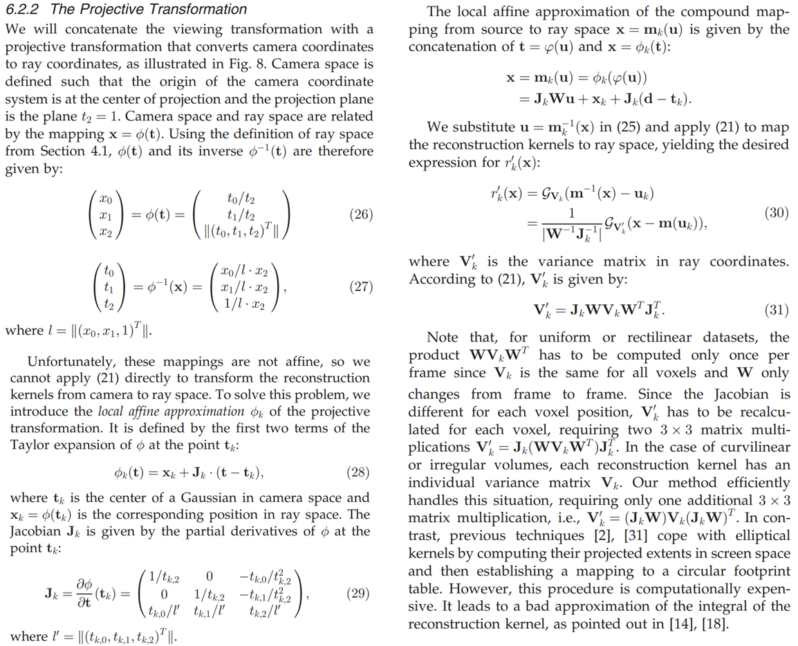
论文中使用了泰勒公式逼近真实的2维Gaussian,具体细节这里不展开。
3. computeCov3D
根据缩放和旋转计算三维协方差矩阵。比较简单。
// Forward method for converting scale and rotation properties of each
// Gaussian to a 3D covariance matrix in world space. Also takes care
// of quaternion normalization.
__device__ void computeCov3D(const glm::vec3 scale, // 表示缩放的三维向量float mod, // 对应gaussian_renderer/__init__.py中的scaling_modifierconst glm::vec4 rot, // 表示旋转的四元数float* cov3D) // 结果:三维协方差矩阵
{// Create scaling matrixglm::mat3 S = glm::mat3(1.0f);S[0][0] = mod * scale.x;S[1][1] = mod * scale.y;S[2][2] = mod * scale.z;// Normalize quaternion to get valid rotationglm::vec4 q = rot;// / glm::length(rot);float r = q.x;float x = q.y;float y = q.z;float z = q.w;// Compute rotation matrix from quaternionglm::mat3 R = glm::mat3(1.f - 2.f * (y * y + z * z), 2.f * (x * y - r * z), 2.f * (x * z + r * y),2.f * (x * y + r * z), 1.f - 2.f * (x * x + z * z), 2.f * (y * z - r * x),2.f * (x * z - r * y), 2.f * (y * z + r * x), 1.f - 2.f * (x * x + y * y));glm::mat3 M = S * R;// Compute 3D world covariance matrix Sigmaglm::mat3 Sigma = glm::transpose(M) * M;// Covariance is symmetric, only store upper rightcov3D[0] = Sigma[0][0];cov3D[1] = Sigma[0][1];cov3D[2] = Sigma[0][2];cov3D[3] = Sigma[1][1];cov3D[4] = Sigma[1][2];cov3D[5] = Sigma[2][2];
}
4. preprocessCUDA
预处理函数,作用是:
// Perform initial steps for each Gaussian prior to rasterization.
template<int C>
__global__ void preprocessCUDA(int P, int D, int M,const float* orig_points, // 也就是CudaRasterizer::Rasterizer::forward的means3Dconst glm::vec3* scales,const float scale_modifier,const glm::vec4* rotations,const float* opacities,const float* shs,bool* clamped,const float* cov3D_precomp,const float* colors_precomp,const float* viewmatrix,const float* projmatrix,const glm::vec3* cam_pos,const int W, int H,const float tan_fovx, float tan_fovy,const float focal_x, float focal_y,int* radii,/*上面这些参数的含义都提到过*/float2* points_xy_image,  // Gaussian中心在图像上的像素坐标float* depths, // Gaussian中心的深度,即其在相机坐标系的z轴的坐标float* cov3Ds, // 三维协方差矩阵float* rgb, // 根据球谐算出的RGB颜色值float4* conic_opacity, // 椭圆对应二次型的矩阵和不透明度的打包存储const dim3 grid, // tile的在x、y方向上的数量uint32_t* tiles_touched, // Gaussian覆盖的tile数量bool prefiltered)
{auto idx = cg::this_grid().thread_rank(); // 该函数预处理第idx个Gaussianif (idx >= P)return;// Initialize radius and touched tiles to 0. If this isn't changed,// this Gaussian will not be processed further.radii[idx] = 0;tiles_touched[idx] = 0;// Perform near culling, quit if outside.float3 p_view; // Gaussian中心在相机坐标系下的坐标if (!in_frustum(idx, orig_points, viewmatrix, projmatrix, prefiltered, p_view))return; // 不在相机的视锥内就不管了// Transform point by projectingfloat3 p_orig = { orig_points[3 * idx], orig_points[3 * idx + 1], orig_points[3 * idx + 2] };float4 p_hom = transformPoint4x4(p_orig, projmatrix); // homogeneous coordinates(齐次坐标)float p_w = 1.0f / (p_hom.w + 0.0000001f); // 想要除以p_hom.w从而转成正常的3D坐标,这里防止除零float3 p_proj = { p_hom.x * p_w, p_hom.y * p_w, p_hom.z * p_w };// If 3D covariance matrix is precomputed, use it, otherwise compute// from scaling and rotation parameters. const float* cov3D;if (cov3D_precomp != nullptr){cov3D = cov3D_precomp + idx * 6;}else{computeCov3D(scales[idx], scale_modifier, rotations[idx], cov3Ds + idx * 6);cov3D = cov3Ds + idx * 6;}// Compute 2D screen-space covariance matrixfloat3 cov = computeCov2D(p_orig, focal_x, focal_y, tan_fovx, tan_fovy, cov3D, viewmatrix);// Invert covariance (EWA algorithm)float det = (cov.x * cov.z - cov.y * cov.y); // 二维协方差矩阵的行列式if (det == 0.0f)return;float det_inv = 1.f / det; // 行列式的逆float3 conic = { cov.z * det_inv, -cov.y * det_inv, cov.x * det_inv };// conic是cone的形容词,意为“圆锥的”。猜测这里是指圆锥曲线(椭圆)。// 二阶矩阵求逆口诀:“主对调,副相反”。// Compute extent in screen space (by finding eigenvalues of// 2D covariance matrix). Use extent to compute a bounding rectangle// of screen-space tiles that this Gaussian overlaps with. Quit if// rectangle covers 0 tiles. float mid = 0.5f * (cov.x + cov.z);float lambda1 = mid + sqrt(max(0.1f, mid * mid - det));float lambda2 = mid - sqrt(max(0.1f, mid * mid - det));// 韦达定理求二维协方差矩阵的特征值float my_radius = ceil(3.f * sqrt(max(lambda1, lambda2)));// 原理见代码后面我的补充说明// 这里就是截取Gaussian的中心部位(3σ原则),只取像平面上半径为my_radius的部分float2 point_image = { ndc2Pix(p_proj.x, W), ndc2Pix(p_proj.y, H) };// ndc2Pix(v, S) = ((v + 1) * S - 1) / 2 = (v + 1) / 2 * S - 0.5uint2 rect_min, rect_max;getRect(point_image, my_radius, rect_min, rect_max, grid);// 检查该Gaussian在图片上覆盖了哪些tile(由一个tile组成的矩形表示)if ((rect_max.x - rect_min.x) * (rect_max.y - rect_min.y) == 0)return; // 不与任何tile相交,不管了// If colors have been precomputed, use them, otherwise convert// spherical harmonics coefficients to RGB color.if (colors_precomp == nullptr){glm::vec3 result = computeColorFromSH(idx, D, M, (glm::vec3*)orig_points, *cam_pos, shs, clamped);rgb[idx * C + 0] = result.x;rgb[idx * C + 1] = result.y;rgb[idx * C + 2] = result.z;}// Store some useful helper data for the next steps.depths[idx] = p_view.z; // 深度,即相机坐标系的z轴radii[idx] = my_radius; // Gaussian在像平面坐标系下的半径// 这里很奇怪,明明radii是int数组为什么赋了一个float值?points_xy_image[idx] = point_image; // Gaussian中心在图像上的像素坐标// Inverse 2D covariance and opacity neatly pack into one float4conic_opacity[idx] = { conic.x, conic.y, conic.z, opacities[idx] };tiles_touched[idx] = (rect_max.y - rect_min.y) * (rect_max.x - rect_min.x);// Gaussian覆盖的tile数量
}
补充说明
❄️(1) 关于二维高斯分布和椭圆的关系,我们可以这么考虑:
二维高斯分布的概率密度函数为 p ( x ) = 1 ( 2 π ) n 2 ∣ Σ ∣ 1 2 exp { − 1 2 ( x − μ ) T Σ − 1 ( x − μ ) } \begin{equation} p(\boldsymbol{x})=\frac{1}{(2\pi)^{\frac{n}{2}}|\Sigma|^{\frac{1}{2}}}\exp\left\{-\frac{1}{2}(\bm{x}-\bm{\mu})^T \Sigma^{-1} (\bm{x}-\bm{\mu})\right\} \tag{†} \end{equation} p(x)=(2π)2n∣Σ∣211exp{−21(x−μ)TΣ−1(x−μ)}(†),其中 x = ( x , y ) T \boldsymbol{x}=(x,y)^T x=(x,y)T, Σ \Sigma Σ为协方差矩阵, μ \mu μ为均值。考虑令 p ( x ) p(\boldsymbol{x}) p(x)等于一个常数,并令 u = x − μ \boldsymbol{u}=\boldsymbol{x}-\boldsymbol{\mu} u=x−μ,即 u T Σ − 1 u = R 2 \boldsymbol{u}^T\Sigma^{-1}\boldsymbol{u}=R^2 uTΣ−1u=R2其中 R 2 R^2 R2为常数。由于 Σ \Sigma Σ是对称矩阵,一定存在正交矩阵 P P P使得 Σ = P T Λ P \Sigma=P^T\Lambda P Σ=PTΛP其中 Λ = diag ( λ 1 , λ 2 ) \Lambda=\operatorname{diag}(\lambda_1,\lambda_2) Λ=diag(λ1,λ2)是由 Σ \Sigma Σ的特征值组成的对角矩阵。带入式 ( † ) (†) (†)得 u T P T Λ − 1 P u = R 2 \boldsymbol{u}^T P^T\Lambda^{-1} P\boldsymbol{u}=R^2 uTPTΛ−1Pu=R2令 v = P u \boldsymbol{v}=P\boldsymbol{u} v=Pu(也就是相对 u \boldsymbol{u} u坐标系旋转了一个角度),则 v T Λ − 1 v = R 2 \boldsymbol{v}^T\Lambda^{-1}\boldsymbol{v}=R^2 vTΛ−1v=R2即 v 1 2 λ 1 R 2 + v 2 2 λ 2 R 2 = 1 \frac{v_1^2}{\lambda_1R^2}+\frac{v_2^2}{\lambda_2 R^2}=1 λ1R2v12+λ2R2v22=1正好是一个长短轴分别为 λ 1 R \sqrt{\lambda_1}R λ1R、 λ 2 R \sqrt{\lambda_2}R λ2R的椭圆。令 R = 3 R=3 R=3就得到了代码中算my_radius的公式。
❄️(2) 关于ndc2Pix的解读:
这时候我们必须知道p_proj的真正含义。p_proj是projmatrix乘以Gaussian中心的世界坐标p_orig的结果。proj_matrix又是W2C矩阵和投影矩阵的积。我们重点关注投影矩阵。计算投影矩阵的函数为utils/graph_utils.py中的getProjectionMatrix:
def getProjectionMatrix(znear, zfar, fovX, fovY):tanHalfFovY = math.tan((fovY / 2))tanHalfFovX = math.tan((fovX / 2))top = tanHalfFovY * znearbottom = -topright = tanHalfFovX * znearleft = -rightP = torch.zeros(4, 4)z_sign = 1.0P[0, 0] = 2.0 * znear / (right - left)P[1, 1] = 2.0 * znear / (top - bottom)P[0, 2] = (right + left) / (right - left)P[1, 2] = (top + bottom) / (top - bottom)P[3, 2] = z_signP[2, 2] = z_sign * zfar / (zfar - znear)P[2, 3] = -(zfar * znear) / (zfar - znear)return P
这个函数写的极其怪异,P[0,2]和P[1,2]显然为 0 0 0,不知道作者的用意是什么。回想znear和zfar代表该相机能看到的最近和最远距离。注意矩阵 P P P是从相机坐标系到像平面二维坐标系的映射,可以表示为 P = [ t a n H a l f F o v X t a n H a l f F o v Y z f a r z f a r − z n e a r z f a r × z n e a r z f a r − z n e a r ] P=\begin{bmatrix} \mathrm{tanHalfFovX} &&&\\ &\mathrm{tanHalfFovY}&&\\ &&\frac{\mathrm{zfar}}{\mathrm{zfar}-\mathrm{znear}}&\frac{\mathrm{zfar}\times\mathrm{znear}}{\mathrm{zfar}-\mathrm{znear}}\\ \end{bmatrix} P= tanHalfFovXtanHalfFovYzfar−znearzfarzfar−znearzfar×znear 所以, P [ x y z ] = [ t a n H a l f F o v X × x t a n H a l f F o v Y × y z f a r ( z − z n e a r ) z f a r − z n e a r ] P\begin{bmatrix}x\\y\\z\end{bmatrix}= \begin{bmatrix} \mathrm{tanHalfFovX}\times x\\ \mathrm{tanHalfFovY}\times y\\ \cfrac{\mathrm{zfar}(z-\mathrm{znear})}{\mathrm{zfar}-\mathrm{znear}} \end{bmatrix} P xyz = tanHalfFovX×xtanHalfFovY×yzfar−znearzfar(z−znear) 显然,作者假设像平面到相机中心的距离为 1 1 1,且相机坐标系的 z z z轴与像平面垂直。 P P P矩阵把 z z z的范围 [ z n e a r , z f a r ] [\mathrm{znear},\mathrm{zfar}] [znear,zfar]映射到 [ 0 , z f a r ] [0,\mathrm{zfar}] [0,zfar]; x , y x,y x,y被映射到了像平面上的坐标,其中图像中心在像平面上的坐标为 ( 0 , 0 ) (0,0) (0,0),图像边缘在像平面上的 x x x、 y y y坐标为 ± 1 \pm 1 ±1。
函数ndc2Pix的作用就是把像平面上的坐标转化为像素坐标。我们提到,ndc2Pix(v, S)等价于(v + 1) / 2 * S - 0.5。首先把范围 [ − 1 , 1 ] [-1,1] [−1,1]映射为 [ 0 , 2 ] [0,2] [0,2],再除以 2 2 2得 [ 0 , 1 ] [0,1] [0,1],乘 S S S(等于图像宽度或高度)就转化为了像素坐标,最后 − 0.5 -0.5 −0.5映射到像素中心。
❗️注意:我们有四个坐标系:世界坐标系、相机坐标系、像平面坐标系、图像坐标系,关系如图:
5. render和renderCUDA
void FORWARD::render(const dim3 grid, dim3 block,const uint2* ranges,const uint32_t* point_list,int W, int H,const float2* means2D,const float* colors,const float4* conic_opacity,float* final_T,uint32_t* n_contrib,const float* bg_color,float* out_color)
{renderCUDA<NUM_CHANNELS> << <grid, block >> > (ranges,point_list,W, H,means2D,colors,conic_opacity,final_T,n_contrib,bg_color,out_color);// 一个线程负责一个像素,一个block负责一个tile
}// Main rasterization method. Collaboratively works on one tile per
// block, each thread treats one pixel. Alternates between fetching
// and rasterizing data.
// "Alternates between fetching and rasterizing data":
// 线程在读取数据(把数据从公用显存拉到block自己的显存)和进行计算之间来回切换,
// 使得线程们可以共同读取Gaussian数据。
// 这样做的原因是block共享内存比公共显存快得多。
template <uint32_t CHANNELS> // CHANNELS取3,即RGB三个通道
__global__ void __launch_bounds__(BLOCK_X * BLOCK_Y)
renderCUDA(const uint2* __restrict__ ranges, // 每个tile对应排过序的数组中的哪一部分const uint32_t* __restrict__ point_list, // 按tile、深度排序后的Gaussian ID列表int W, int H, // 图像宽高const float2* __restrict__ points_xy_image, // 图像上每个Gaussian中心的2D坐标const float* __restrict__ features, // RGB颜色const float4* __restrict__ conic_opacity, // 解释过了float* __restrict__ final_T, // 最终的透光率uint32_t* __restrict__ n_contrib,// 多少个Gaussian对该像素的颜色有贡献(用于反向传播时判断各个Gaussian有没有梯度)const float* __restrict__ bg_color, // 背景颜色float* __restrict__ out_color) // 渲染结果(图片)
{// Identify current tile and associated min/max pixel range.auto block = cg::this_thread_block();uint32_t horizontal_blocks = (W + BLOCK_X - 1) / BLOCK_X; // x方向上tile的个数uint2 pix_min = { block.group_index().x * BLOCK_X, block.group_index().y * BLOCK_Y };// 我负责的tile的坐标较小的那个角的坐标uint2 pix_max = { min(pix_min.x + BLOCK_X, W), min(pix_min.y + BLOCK_Y , H) };// 我负责的tile的坐标较大的那个角的坐标uint2 pix = { pix_min.x + block.thread_index().x, pix_min.y + block.thread_index().y };// 我负责哪个像素uint32_t pix_id = W * pix.y + pix.x;// 我负责的像素在整张图片中排行老几float2 pixf = { (float)pix.x, (float)pix.y }; // pix的浮点数版本// Check if this thread is associated with a valid pixel or outside.bool inside = pix.x < W && pix.y < H; // 看看我负责的像素有没有跑到图像外面去// Done threads can help with fetching, but don't rasterizebool done = !inside;// Load start/end range of IDs to process in bit sorted list.uint2 range = ranges[block.group_index().y * horizontal_blocks + block.group_index().x];const int rounds = ((range.y - range.x + BLOCK_SIZE - 1) / BLOCK_SIZE);// BLOCK_SIZE = 16 * 16 = 256// 我要把任务分成rounds批,每批处理BLOCK_SIZE个Gaussians// 每一批,每个线程负责读取一个Gaussian的信息,// 所以该block的256个线程每一批就可以读取256个Gaussian的信息int toDo = range.y - range.x; // 我要处理的Gaussian个数// Allocate storage for batches of collectively fetched data.// __shared__: 同一block中的线程共享的内存__shared__ int collected_id[BLOCK_SIZE];__shared__ float2 collected_xy[BLOCK_SIZE];__shared__ float4 collected_conic_opacity[BLOCK_SIZE];// Initialize helper variablesfloat T = 1.0f; // T = transmittance,透光率uint32_t contributor = 0; // 多少个Gaussian对该像素的颜色有贡献uint32_t last_contributor = 0; // 比contributor慢半拍的变量float C[CHANNELS] = { 0 }; // 渲染结果// Iterate over batches until all done or range is completefor (int i = 0; i < rounds; i++, toDo -= BLOCK_SIZE){// End if entire block votes that it is done rasterizingint num_done = __syncthreads_count(done);// 它首先具有__syncthreads的功能(让所有线程回到同一个起跑线上),// 并且返回对于多少个线程来说done是true。if (num_done == BLOCK_SIZE)break; // 全干完了,收工// Collectively fetch per-Gaussian data from global to shared// 由于当前block的线程要处理同一个tile,所以它们面对的Gaussians也是相同的// 因此合作读取BLOCK_SIZE条的数据。// 之所以分批而不是一次读完可能是因为block的共享内存空间有限。int progress = i * BLOCK_SIZE + block.thread_rank();if (range.x + progress < range.y) // 我还有没有活干{// 读取我负责的Gaussian信息int coll_id = point_list[range.x + progress];collected_id[block.thread_rank()] = coll_id;collected_xy[block.thread_rank()] = points_xy_image[coll_id];collected_conic_opacity[block.thread_rank()] = conic_opacity[coll_id];}block.sync(); // 这下collected_*** 数组就被填满了// Iterate over current batchfor (int j = 0; !done && j < min(BLOCK_SIZE, toDo); j++){// Keep track of current position in rangecontributor++;// 下面计算当前Gaussian的不透明度// Resample using conic matrix (cf. "Surface // Splatting" by Zwicker et al., 2001)float2 xy = collected_xy[j]; // Gaussian中心float2 d = { xy.x - pixf.x, xy.y - pixf.y };// 该像素到Gaussian中心的位移向量float4 con_o = collected_conic_opacity[j];float power = -0.5f * (con_o.x * d.x * d.x + con_o.z * d.y * d.y) - con_o.y * d.x * d.y;// 二维高斯分布公式的指数部分(见补充说明)if (power > 0.0f)continue;// Eq. (2) from 3D Gaussian splatting paper.// Obtain alpha by multiplying with Gaussian opacity// and its exponential falloff from mean.// Avoid numerical instabilities (see paper appendix). float alpha = min(0.99f, con_o.w * exp(power));// Gaussian对于这个像素点来说的不透明度// 注意con_o.w是”opacity“,是Gaussian整体的不透明度if (alpha < 1.0f / 255.0f) // 不透明度太小,不渲染continue;float test_T = T * (1 - alpha); // 透光率是累乘if (test_T < 0.0001f){ // 当透光率很低的时候,就不继续渲染了(反正渲染了也看不见)done = true;continue;}// Eq. (3) from 3D Gaussian splatting paper.for (int ch = 0; ch < CHANNELS; ch++)C[ch] += features[collected_id[j] * CHANNELS + ch] * alpha * T;// 计算当前Gaussian对像素颜色的贡献T = test_T; // 更新透光率// Keep track of last range entry to update this// pixel.last_contributor = contributor;}}// All threads that treat valid pixel write out their final// rendering data to the frame and auxiliary buffers.if (inside){final_T[pix_id] = T;n_contrib[pix_id] = last_contributor;for (int ch = 0; ch < CHANNELS; ch++)out_color[ch * H * W + pix_id] = C[ch] + T * bg_color[ch];// 把渲染出来的像素值写进out_color}
}
补充说明
二维高斯分布的指数部分为 − 1 2 d T Σ − 1 d -\frac{1}{2}\boldsymbol{d}^T\Sigma^{-1}\boldsymbol{d} −21dTΣ−1d其中 d \boldsymbol{d} d就是代码中的d(像素到Gaussian中心的位移向量), Σ − 1 = [ c o n _ o . x c o n _ o . y c o n _ o . y c o n _ o . z ] \Sigma^{-1}=\begin{bmatrix}\mathtt{con\_o.x}&\mathtt{con\_o.y}\\\mathtt{con\_o.y}&\mathtt{con\_o.z}\end{bmatrix} Σ−1=[con_o.xcon_o.ycon_o.ycon_o.z]。把矩阵乘开就得到了代码中的-0.5f * (con_o.x * d.x * d.x + con_o.z * d.y * d.y) - con_o.y * d.x * d.y。
至于为什么不乘前面的常数 1 ( 2 π ) n 2 ∣ Σ ∣ 1 2 \frac{1}{(2\pi)^{\frac{n}{2}}|\Sigma|^{\frac{1}{2}}} (2π)2n∣Σ∣211呢?因为con_o.w(即opacity)是可学习的参数,这个常量可以包括进去。
下一部分:【计算机视觉】Gaussian Splatting源码解读补充(三)
相关文章:
【计算机视觉】Gaussian Splatting源码解读补充(二)
第一部分 本文是对学习笔记之——3D Gaussian Splatting源码解读的补充,并订正了一些错误。 目录 三、相机相关scene/cameras.py:class Camera 四、前向传播(渲染):submodules/diff-gaussian-rasterization/cuda_rast…...
Java transient 关键字
Java字段不想序列化怎么办 在 Java 中,如果某个字段不想被序列化(即不希望被写入到序列化的数据流中),可以使用 transient 关键字进行标记。通过在字段前加上 transient 关键字,可以告诉 Java 序列化机制忽略该字段&am…...
邂逅Webpack和打包过程)
前端工程化(三)邂逅Webpack和打包过程
目录 Vue项目加载Webpack 安装Webpack的默认打包创建局部的 webpack Vue项目加载 JavaScript的打包: 将ES6转换成ES5的语法; TypeScript的处理,将其转换成JavaScript; Css的处理: CSS文件模块的加载、提取&a…...

Gradle v8.5 笔记 - 从入门到进阶(基于 Kotlin DSL)
目录 一、前置说明 二、Gradle 启动! 2.1、安装 2.2、初始化项目 2.3、gradle 项目目录介绍 2.4、Gradle 项目下载慢?(万能解决办法) 2.5、Gradle 常用命令 2.6、项目构建流程 2.7、设置文件(settings.gradle…...
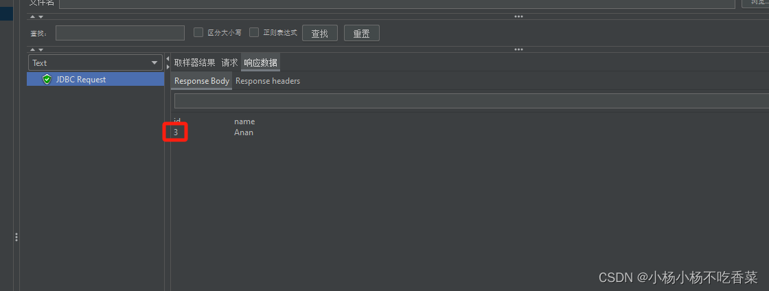
Jmeter-基础元件使用(二)-属性及对数据库简单操作
一、Jmeter属性 当我们想要在不同线程组中使用某变量,就需要使用属,此时Jmeter属性的设置需要函数来进行set和get操作 1.创建set函数 2.然后采用Beanshell取样器进行函数执行 3.调用全局变量pro_id 4.将上面生成的函数字符串粘贴到另一个线程组即可…...
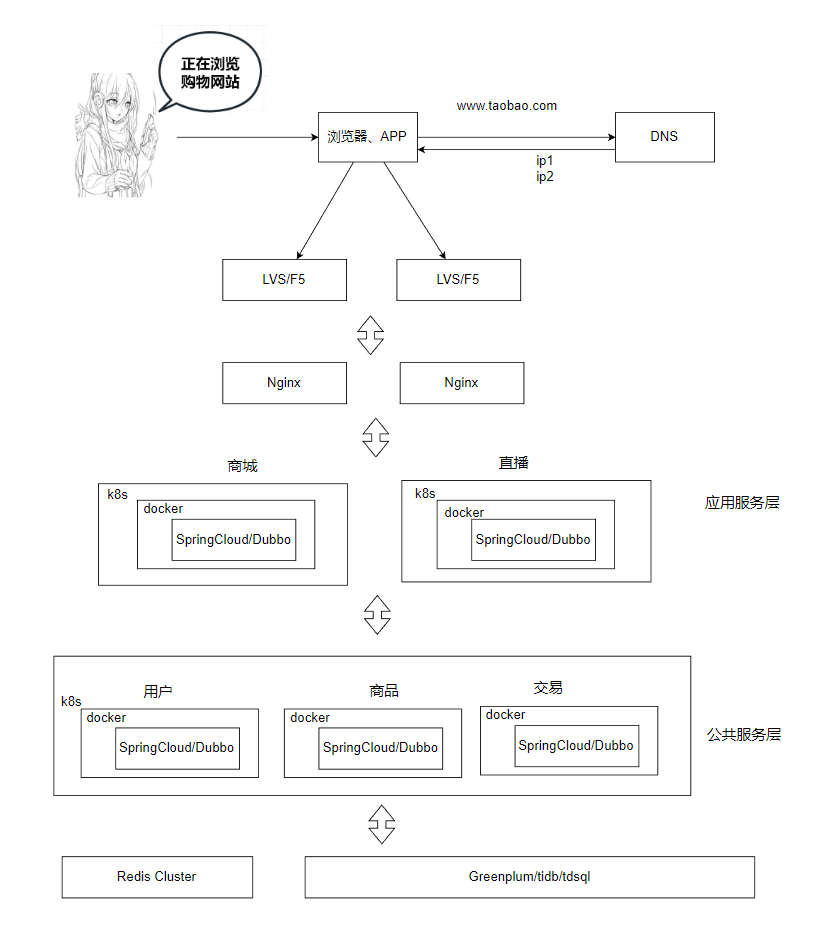
docker 的八大技术架构(图解)
docker 的八大技术架构 单机架构 概念: 应用服务和数据库服务公用一台服务器 出现背景: 出现在互联网早期,访问量比较小,单机足以满足需求 架构优缺点: 优点:部署简单,成本低 缺点࿱…...

LeetCode-热题100:131. 分割回文串
题目描述 给你一个字符串 s,请你将 s 分割成一些子串,使每个子串都是 回文串 。返回 s 所有可能的分割方案。 示例 1: 输入: s “aab” 输出: [[“a”,“a”,“b”],[“aa”,“b”]] 示例 2: 输入&am…...
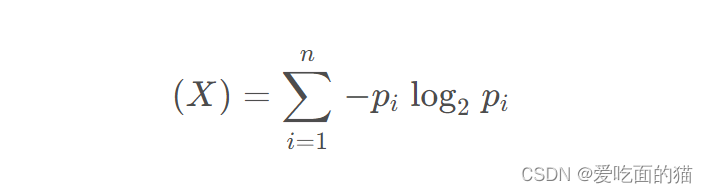
常用相似度计算方法总总结
一、欧几里得相似度 1、欧几里得相似度 公式如下所示: 2、自定义代码实现 import numpy as np def EuclideanDistance(x, y):import numpy as npx np.array(x)y np.array(y)return np.sqrt(np.sum(np.square(x-y)))# 示例数据 # 用户1 的A B C D E商品数据 [3.3…...
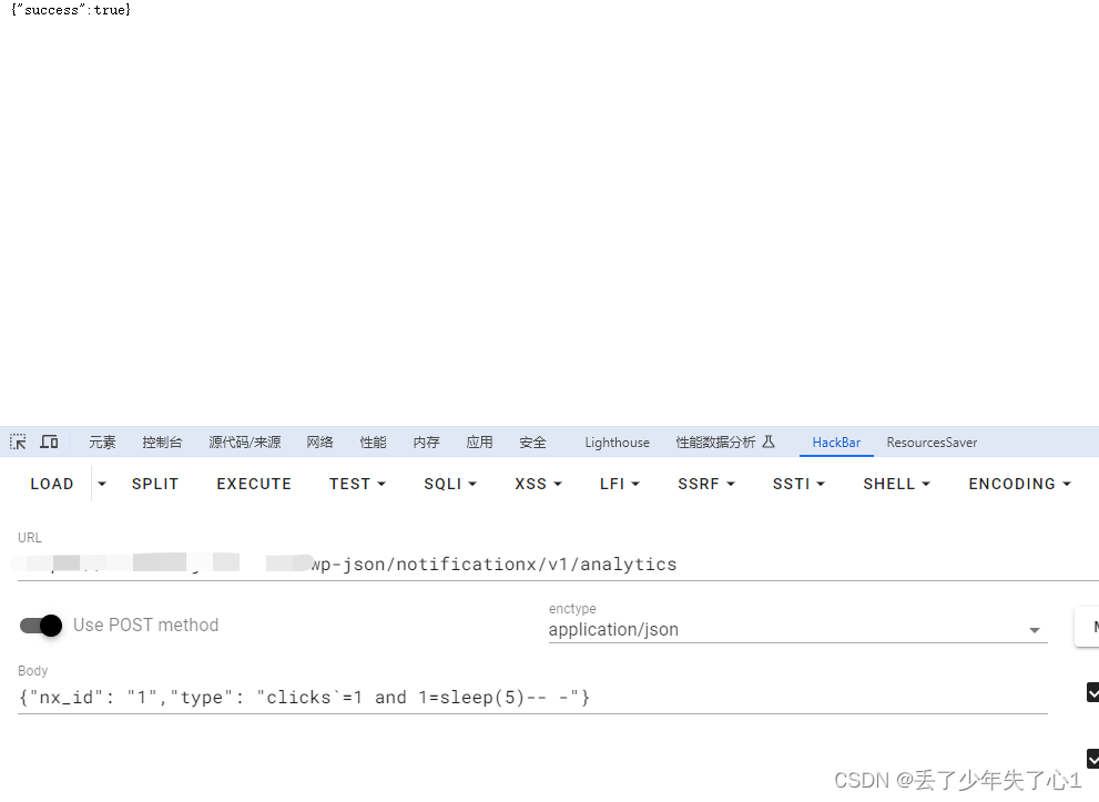
【漏洞复现】WordPress Plugin NotificationX 存在sql注入CVE-2024-1698
漏洞描述 WordPress和WordPress plugin都是WordPress基金会的产品。WordPress是一套使用PHP语言开发的博客平台。该平台支持在PHP和MySQL的服务器上架设个人博客网站。WordPress plugin是一个应用插件。 WordPress Plugin NotificationX 存在安全漏洞,该漏洞源于对用户提供的…...

AI新工具(20240322) 免费试用Gemini Pro 1.5;先进的AI软件工程师Devika;人形机器人Apptronik给你打果汁
✨ 1: Gemini Pro 1.5 免费试用Gemini Pro 1.5 Gemini 1.5 Pro是Gemini系列模型的最新版本,是一种计算高效的多模态混合专家(MoE)模型。它能够从数百万个上下文Token中提取和推理细粒度信息,包括多个长文档和数小时的视频、音频…...
)
鬼灭之刃-激情台词-02(解释来自文心一言)
愤怒吧,不共戴天的仇恨,强悍而纯粹的愤怒,将会化作坚不可摧的原动力,督促你变强 —— 吾峠呼世晴《鬼灭之刃》 愤怒和仇恨是一种强烈的情感,它们可以驱使人们去寻求改变,去变得更加强大。在故事中ÿ…...

openssl3.2 - exp - aes-128-cbc
文章目录 openssl3.2 - exp - aes-128-cbc概述笔记openssl 命令行实现简单直白的实现简单直白的实现 - 测试效果简单直白的实现 - 测试工程 周全灵活的实现周全灵活的实现 - 测试效果周全灵活的实现 - 测试工程 清晰一些的版本END openssl3.2 - exp - aes-128-cbc 概述 想将工…...

基于docker+rancher部署Vue项目的教程
基于dockerrancher部署Vue的教程 前段时间总有前端开发问我Vue如何通过docker生成镜像,并用rancher上进行部署?今天抽了2个小时研究了一下,给大家记录一下这个过程。该部署教程适用于Vue、Vue2、Vue3等版本。 PS:该教程基于有一定…...

Elasticsearch:让你的 Elasticsearch 索引与 Python 和 Google Cloud Platform 功能保持同步
作者:来自 Elastic Garson Elasticsearch 内的索引 (index) 是你可以将数据存储在文档中的位置。 在使用索引时,如果你使用的是动态数据集,数据可能会很快变旧。 为了避免此问题,你可以创建一个 Python 脚本来更新索引࿰…...

如何定位web前后台的BUG
一、对系统整体的了解 Server端:jspServletjson 数据库:sql、MySQL、oracle等 前台: 涉及到 jstl,jsp,js,css,htm等方面 后台:servlet,jms,ejb࿰…...

谈谈 IOC 和 AOP
我之前面试的时候,真的会有面试官问这个。我感觉确实这个比较高频,因为 Spring 框架最核心的就是这两个东西嘛,掌握了这两个就相当于掌握了 Spring 的半壁江山了。 不过一般面试官不会一上来就问你什么是 AOP 和 IOC,一般都是叫你…...

C/C++之内存旋律:星辰大海的指挥家
个人主页:日刷百题 系列专栏:〖C/C小游戏〗〖Linux〗〖数据结构〗 〖C语言〗 🌎欢迎各位→点赞👍收藏⭐️留言📝 一、C/C内存分布 我们先来了解一下C/C内存分配的几个区域,以下面的代码为例来看…...

Linux下进程的调度与切换
🌎进程的调度与切换 文章目录: 进程的调度与切换 进程切换 进程调度 活动状态进程队列 位图判断 过期队列 总结 前言: 在Linux操作系统中,进程的调度与切换是操作系统核心功能之一ÿ…...
Linux相关命令(2)
1、W :主要是查看当前登录的用户 在上面这个截图里面呢, 第一列 user ,代表登录的用户, 第二列, tty 代表用户登录的终端号,因为在 linux 中并不是只有一个终端的, pts/2 代表是图形界面的第…...

React中 类组件 与 函数组件 的区别
类组件 与 函数组件 的区别 1. 类组件2. 函数组件HookuseStateuseEffectuseCallbackuseMemouseContextuseRef 3. 函数组件与类组件的区别3.1 表面差异3.2 最大不同原因 1. 类组件 在React中,类组件就是基于ES6语法,通过继承 React.component 得到的组件…...

IPFS去中心化存储实战指南:黑马程序员音乐播放器项目开发完整教程
IPFS去中心化存储实战指南:黑马程序员音乐播放器项目开发完整教程 【免费下载链接】BlockChain 黑马程序员 120天全栈区块链开发 开源教程 项目地址: https://gitcode.com/gh_mirrors/blockchain95/BlockChain 你是否想过如何构建一个真正去中心化的音乐播放…...

Buzz音频转录完全指南:3大核心功能+5个实战场景,快速掌握本地语音转文字技术
Buzz音频转录完全指南:3大核心功能5个实战场景,快速掌握本地语音转文字技术 【免费下载链接】buzz Buzz transcribes and translates audio offline on your personal computer. Powered by OpenAIs Whisper. 项目地址: https://gitcode.com/GitHub_Tr…...

告别沉浸式白屏!UniApp中iOS/Android底部安全区与顶部状态栏颜色自定义全攻略
告别沉浸式白屏!UniApp中iOS/Android底部安全区与顶部状态栏颜色自定义全攻略当开发者尝试在UniApp中实现沉浸式设计时,往往会遇到一个令人头疼的问题——默认的白色安全区和状态栏导致界面元素(如电池图标、信号强度)几乎不可见。…...

新手也能懂的SSRF漏洞实战:用iwebsec靶场复现文件读取与内网探测
从零开始掌握SSRF漏洞:iwebsec靶场实战指南1. 认识SSRF漏洞的本质想象一下,你正在一家高档餐厅点餐,服务员承诺可以帮你从任何地方获取食材——包括隔壁竞争对手的厨房。SSRF(Server-Side Request Forgery)漏洞就像这个…...
)
ParaView时间戳设置全攻略:从基础标注到自定义格式(5.8.0实测)
ParaView时间戳设置全攻略:从基础标注到自定义格式(5.8.0实测) 在科学可视化领域,时间戳不仅是数据演变的见证者,更是研究成果呈现的专业语言。ParaView作为开源可视化工具链的标杆,其时间标注功能在学术论…...

CANN-昇腾NPU-RAG推理-检索增强生成怎么部署
RAG(Retrieval-Augmented Generation)是 LLM 知识库的组合:先检索相关文档,再让 LLM 基于文档回答。昇腾NPU 上部署 RAG 需要两个组件:Embedding 模型(做向量检索)和 LLM(做生成&am…...

AI时代程序员职业发展与个人创业可行性研究报告
一、行业宏观变革(2026核心趋势数据佐证) 1.1 开发范式已彻底重构(行业不可逆拐点) 2026年正式进入AI Agent智能体开发时代,传统CRUD编码价值持续崩塌。 核心权威数据: Gartner预测:2026年75%企…...

MobX社区资源大全:10个必备工具、插件和扩展库推荐 [特殊字符]
MobX社区资源大全:10个必备工具、插件和扩展库推荐 🚀 【免费下载链接】MobX-Docs-CN MobX 中文文档 项目地址: https://gitcode.com/gh_mirrors/mo/MobX-Docs-CN MobX作为一个简单、可扩展的状态管理库,已经成为React开发者不可或缺的…...

CSharpVerbalExpressions常见问题解答:解决开发者遇到的10个典型挑战
CSharpVerbalExpressions常见问题解答:解决开发者遇到的10个典型挑战 【免费下载链接】CSharpVerbalExpressions 项目地址: https://gitcode.com/gh_mirrors/cs/CSharpVerbalExpressions CSharpVerbalExpressions是一个强大的C#库,它通过类自然语…...

AutoWall终极指南:如何在Windows上轻松设置炫酷动态壁纸
AutoWall终极指南:如何在Windows上轻松设置炫酷动态壁纸 【免费下载链接】AutoWall 🌌 Live wallpapers on Windows 7/8/10/11 using open-source wallpaper engine 项目地址: https://gitcode.com/gh_mirrors/au/AutoWall 厌倦了千篇一律的静态桌…...