数据挖掘入门项目二手交易车价格预测之建模调参
文章目录
- 目标
- 步骤
- 1. 调整数据类型,减少数据在内存中占用的空间
- 2. 使用线性回归来简单建模
- 3. 五折交叉验证
- 4. 模拟真实业务情况
- 5. 绘制学习率曲线与验证曲线
- 6. 嵌入式特征选择
- 6. 非线性模型
- 7. 模型调参
- (1) 贪心调参
- (2)Grid Search 调参
- (3)贝叶斯调参
- 总结
本文数据集来自阿里天池:https://tianchi.aliyun.com/competition/entrance/231784/information
主要参考了Datawhale的整个操作流程:https://tianchi.aliyun.com/notebook/95460
小编也是第一次接触数据挖掘,所以先跟着Datawhale写的教程操作了一遍,不懂的地方加了一点点自己的理解,感谢Datawhale!
目标
了解常用的机器学习模型,并掌握机器学习模型的建模与调参流程
步骤
1. 调整数据类型,减少数据在内存中占用的空间
具体方法定义如下:
对每一列循环,将每一列的转化为对应的数据类型,在不损失数据的情况下,尽可能地减少DataFrame中每列的内存占用
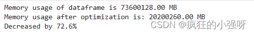
def reduce_mem_usage(df):""" iterate through all the columns of a dataframe and modify the data typeto reduce memory usage. """start_mem = df.memory_usage().sum() # memory_usage() 方法返回每一列的内存使用情况,sum() 将它们相加。print('Memory usage of dataframe is {:.2f} MB'.format(start_mem))# 对每一列循环for col in df.columns:col_type = df[col].dtype # 获取列类型if col_type != object:# 获取当前列的最小值和最大值c_min = df[col].min()c_max = df[col].max()if str(col_type)[:3] == 'int':# np.int8 是 NumPy 中表示 8 位整数的数据类型。# np.iinfo(np.int8) 返回一个描述 np.int8 数据类型的信息对象。# .min 是该信息对象的一个属性,用于获取该数据类型的最小值。if c_min > np.iinfo(np.int8).min and c_max < np.iinfo(np.int8).max:df[col] = df[col].astype(np.int8)elif c_min > np.iinfo(np.int16).min and c_max < np.iinfo(np.int16).max:df[col] = df[col].astype(np.int16)elif c_min > np.iinfo(np.int32).min and c_max < np.iinfo(np.int32).max:df[col] = df[col].astype(np.int32)elif c_min > np.iinfo(np.int64).min and c_max < np.iinfo(np.int64).max:df[col] = df[col].astype(np.int64) else:if c_min > np.finfo(np.float16).min and c_max < np.finfo(np.float16).max:df[col] = df[col].astype(np.float16)elif c_min > np.finfo(np.float32).min and c_max < np.finfo(np.float32).max:df[col] = df[col].astype(np.float32)else:df[col] = df[col].astype(np.float64)else:df[col] = df[col].astype('category') # 将当前列的数据类型转换为分类类型,以节省内存end_mem = df.memory_usage().sum() print('Memory usage after optimization is: {:.2f} MB'.format(end_mem))print('Decreased by {:.1f}%'.format(100 * (start_mem - end_mem) / start_mem))return df
调用上述函数查看效果:
其中,data_for_tree.csv保存的是我们在特征工程步骤中简单处理过的特征
sample_feature = reduce_mem_usage(pd.read_csv('data_for_tree.csv'))
2. 使用线性回归来简单建模
因为上述特征当时是为树模型分析保存的,所以没有对空值进行处理,这里简单处理一下
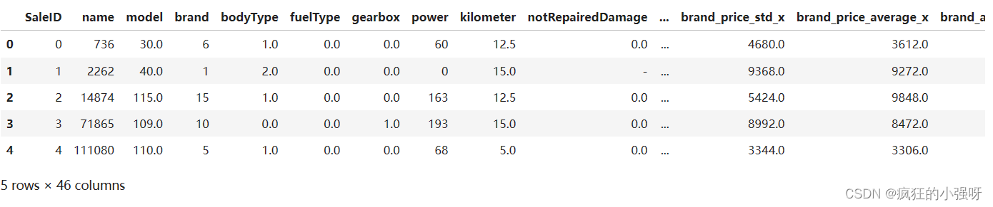
sample_feature.head()
可以看到notRepairedDamage这一列有异常值‘-’:
sample_feature = sample_feature.dropna().replace('-', 0).reset_index(drop=True)
sample_feature['notRepairedDamage'] = sample_feature['notRepairedDamage'].astype(np.float32)
建立训练数据和标签:
train_X = sample_feature.drop('price',axis=1)
train_y = sample_feature['price']
简单建模:
from sklearn.linear_model import LinearRegression
model = LinearRegression()
model = model.fit(train_X, train_y)
'intercept:'+ str(model.intercept_) # 这一行代码用于输出模型的截距(即常数项)
sorted(dict(zip(sample_feature.columns, model.coef_)).items(), key=lambda x:x[1], reverse=True) # 这行代码是用于输出模型的系数,并按照系数的大小进行排序
# sample_feature.columns 是特征的列名。
# model.coef_ 是线性回归模型的系数。
# zip(sample_feature.columns, model.coef_) 将特征列名与对应的系数打包成元组。
# dict(...) 将打包好的元组转换为字典。
# sorted(..., key=lambda x:x[1], reverse=True) 对字典按照值(系数)进行降序排序。
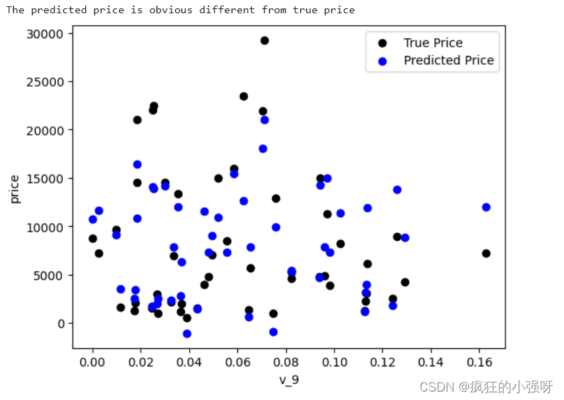
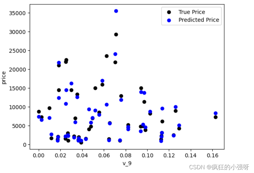
画图查看真实值与预测值之间的差距:
from matplotlib import pyplot as plt
subsample_index = np.random.randint(low=0, high=len(train_y), size=50) # 从训练数据中随机选择 50 个样本的索引
plt.scatter(train_X['v_9'][subsample_index], train_y[subsample_index], color='black') # 绘制真实价格与特征 'v_9' 之间的散点图
plt.scatter(train_X['v_9'][subsample_index], model.predict(train_X.loc[subsample_index]), color='blue') # 绘制模型预测价格与特征 'v_9' 之间的散点图
plt.xlabel('v_9')
plt.ylabel('price')
plt.legend(['True Price','Predicted Price'],loc='upper right')
print('The predicted price is obvious different from true price')
plt.show()
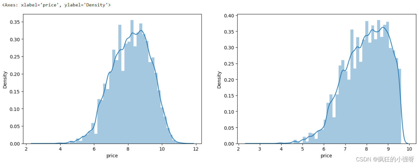
通过作图我们发现数据的标签(price)呈现长尾分布,不利于我们的建模预测。
对标签进行进一步分析:
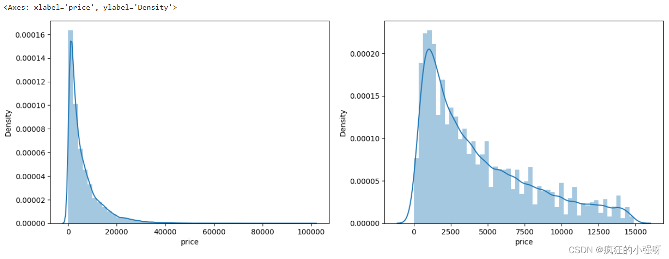
画图显示标签的分布:左边是所有标签数据的一个分布,右边是去掉最大的10%标签数据之后的一个分布
import seaborn as sns
print('It is clear to see the price shows a typical exponential distribution')
plt.figure(figsize=(15,5))
plt.subplot(1,2,1) # 创建一个包含 1 行 2 列的子图,并将当前子图设置为第一个子图
sns.distplot(train_y) # 显示价格数据的直方图以及拟合的密度曲线
plt.subplot(1,2,2)
# quantile 函数来计算价格数据的第 90%分位数,然后通过布尔索引选取低于第 90 百分位数的价格数据
sns.distplot(train_y[train_y < np.quantile(train_y, 0.9)])
对标签进行 log(x+1) 变换,使标签贴近于正态分布:
train_y_ln = np.log(train_y + 1)
显示log变化之后的数据分布:
import seaborn as sns
print('The transformed price seems like normal distribution')
plt.figure(figsize=(15,5))
plt.subplot(1,2,1)
sns.distplot(train_y_ln)
plt.subplot(1,2,2)
sns.distplot(train_y_ln[train_y_ln < np.quantile(train_y_ln, 0.9)])
然后我们重新训练,再可视化
model = model.fit(train_X, train_y_ln)
print('intercept:'+ str(model.intercept_))
sorted(dict(zip(continuous_feature_names, model.coef_)).items(), key=lambda x:x[1], reverse=True)
plt.scatter(train_X['v_9'][subsample_index], train_y[subsample_index], color='black')
plt.scatter(train_X['v_9'][subsample_index], np.exp(model.predict(train_X.loc[subsample_index])), color='blue')
plt.xlabel('v_9')
plt.ylabel('price')
plt.legend(['True Price','Predicted Price'],loc='upper right')
print('The predicted price seems normal after np.log transforming')
plt.show()
可以看出结果要比上面的好一点:
3. 五折交叉验证
在使用训练集对参数进行训练的时候,一般会将整个训练集分为三个部分:训练集(train_set),评估集(valid_set),测试集(test_set)这三个部分。这其实是为了保证训练效果而特意设置的。
- 测试集很好理解,其实就是完全不参与训练的数据,仅仅用来观测测试效果的数据。
- 在实际的训练中,训练的结果对于训练集的拟合程度通常还是挺好的(初始条件敏感),但是对于训练集之外的数据的拟合程度通常就不那么令人满意了。因此我们通常并不会把所有的数据集都拿来训练,而是分出一部分来(这一部分不参加训练)对训练集生成的参数进行测试,相对客观的判断这些参数对训练集之外的数据的符合程度。这种思想就称为交叉验证(Cross Validation)
(1)使用线性回归模型,对未处理标签的特征数据进行五折交叉验证
from sklearn.model_selection import cross_val_score
from sklearn.metrics import mean_absolute_error,  make_scorer
# 下面这个函数主要实现对参数进行对数转换输入目标函数
def log_transfer(func):def wrapper(y, yhat):# np.nan_to_num 函数用于将对数转换后可能出现的 NaN 值转换为 0result = func(np.log(y), np.nan_to_num(np.log(yhat)))return result# 返回内部函数 wrapper,这是一个对原始函数的包装器,它将对传入的参数进行对数转换后再调用原始函数return wrapper
# 计算5折交叉验证得分
scores = cross_val_score(model, X=train_X, y=train_y, verbose=1, cv = 5, scoring=make_scorer(log_transfer(mean_absolute_error)))
# model 是要评估的模型对象。
# train_X 是训练数据的特征,train_y 是训练数据的目标变量。
# verbose=1 设置为 1 时表示打印详细信息。
# cv=5 表示进行 5 折交叉验证。
# scoring=make_scorer(log_transfer(mean_absolute_error)) 指定了评分标准
# 使用了 make_scorer 函数将一个自定义的评分函数 log_transfer(mean_absolute_error) 转换为一个可用于评分的评估器。
# log_transfer(mean_absolute_error) 这一步的作用就是将真实值和预测值在输入到mean_absolute_error之前进行log转换
# mean_absolute_error 是一个回归问题中常用的评估指标,用于衡量预测值与实际值之间的平均绝对误差
print('AVG:', np.mean(scores))
结果展示:

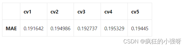
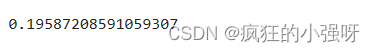
使用线性回归模型,对处理过标签的特征数据进行五折交叉验证:
scores = cross_val_score(model, X=train_X, y=train_y_ln, verbose=1, cv = 5, scoring=make_scorer(mean_absolute_error))
print('AVG:', np.mean(scores))
结果展示:

可以看见,调整之后的数据,误差明显变小
查看scores:
scores = pd.DataFrame(scores.reshape(1,-1))
scores.columns = ['cv' + str(x) for x in range(1, 6)]
scores.index = ['MAE']
scores
4. 模拟真实业务情况
交叉验证在某些与时间相关的数据集上可能反映了不真实的情况,比如我们不能通过2018年的二手车价格来预测2017年的二手车价格。这个时候我们可以采用时间顺序对数据集进行分隔。在本例中,我们可以选用靠前时间的4/5样本当作训练集,靠后时间的1/5当作验证集
具体操作如下:
import datetime
sample_feature = sample_feature.reset_index(drop=True)
split_point = len(sample_feature) // 5 * 4
train = sample_feature.loc[:split_point].dropna()
val = sample_feature.loc[split_point:].dropna()
train_X = train.drop('price',axis=1)
train_y_ln = np.log(train['price'] + 1)
val_X = val.drop('price',axis=1)
val_y_ln = np.log(val['price'] + 1)
model = model.fit(train_X, train_y_ln)
mean_absolute_error(val_y_ln, model.predict(val_X))
结果展示:
5. 绘制学习率曲线与验证曲线
def plot_learning_curve(estimator, title, X, y, ylim=None, cv=None,n_jobs=1, train_size=np.linspace(.1, 1.0, 5 )): """模型估计器 estimator图的标题 title特征数据 X目标数据 yy轴的范围 ylim交叉验证分割策略 cv并行运行的作业数 n_jobs 训练样本的大小 train_size"""plt.figure()  plt.title(title)  if ylim is not None:  plt.ylim(*ylim)  # 设置 y 轴的范围为 ylimplt.xlabel('Training example')  plt.ylabel('score')  # 使用 learning_curve 函数计算学习曲线的训练集得分和交叉验证集得分train_sizes, train_scores, test_scores = learning_curve(estimator, X, y, cv=cv, n_jobs=n_jobs, train_sizes=train_size, scoring = make_scorer(mean_absolute_error))  train_scores_mean = np.mean(train_scores, axis=1)  # 计算训练集得分的均值train_scores_std = np.std(train_scores, axis=1)  # 计算训练集得分的标准差test_scores_mean = np.mean(test_scores, axis=1)  test_scores_std = np.std(test_scores, axis=1)  plt.grid()#区域  # 使用红色填充训练集得分的方差范围plt.fill_between(train_sizes, train_scores_mean - train_scores_std,  train_scores_mean + train_scores_std, alpha=0.1,  color="r")  # 使用绿色填充交叉验证集得分的方差范围plt.fill_between(train_sizes, test_scores_mean - test_scores_std,  test_scores_mean + test_scores_std, alpha=0.1,  color="g")  # 绘制训练集得分曲线plt.plot(train_sizes, train_scores_mean, 'o-', color='r',  label="Training score")  # 绘制交叉验证集得分曲线plt.plot(train_sizes, test_scores_mean,'o-',color="g",  label="Cross-validation score")  plt.legend(loc="best")  return plt
plot_learning_curve(LinearRegression(), 'Liner_model', train_X[:1000], train_y_ln[:1000], ylim=(0.0, 0.5), cv=5, n_jobs=1)
6. 嵌入式特征选择
在过滤式和包裹式特征选择方法中,特征选择过程与学习器训练过程有明显的分别。而嵌入式特征选择在学习器训练过程中自动地进行特征选择。嵌入式选择最常用的是L1正则化与L2正则化。在对线性回归模型加入两种正则化方法后,他们分别变成了岭回归与Lasso回归
对上述三种模型进行交叉验证训练,并对比结果:
from sklearn.linear_model import LinearRegression
from sklearn.linear_model import Ridge
from sklearn.linear_model import Lasso
# 创建一个模型实力列表
models = [LinearRegression(),Ridge(),Lasso()]
result = dict()
for model in models:model_name = str(model)[:-2] # 获取模型名称# 训练模型scores = cross_val_score(model, X=train_X, y=train_y_ln, verbose=0, cv = 5, scoring=make_scorer(mean_absolute_error))# 收集各模型训练得分result[model_name] = scoresprint(model_name + ' is finished')
result = pd.DataFrame(result)
result.index = ['cv' + str(x) for x in range(1, 6)]
result
结果展示:
分别对三个模型训练得到的参数进行分析:
- 一般线性回归
import seaborn as sns
model = LinearRegression().fit(train_X, train_y_ln)
print('intercept:', model.intercept_)
# 组合数据
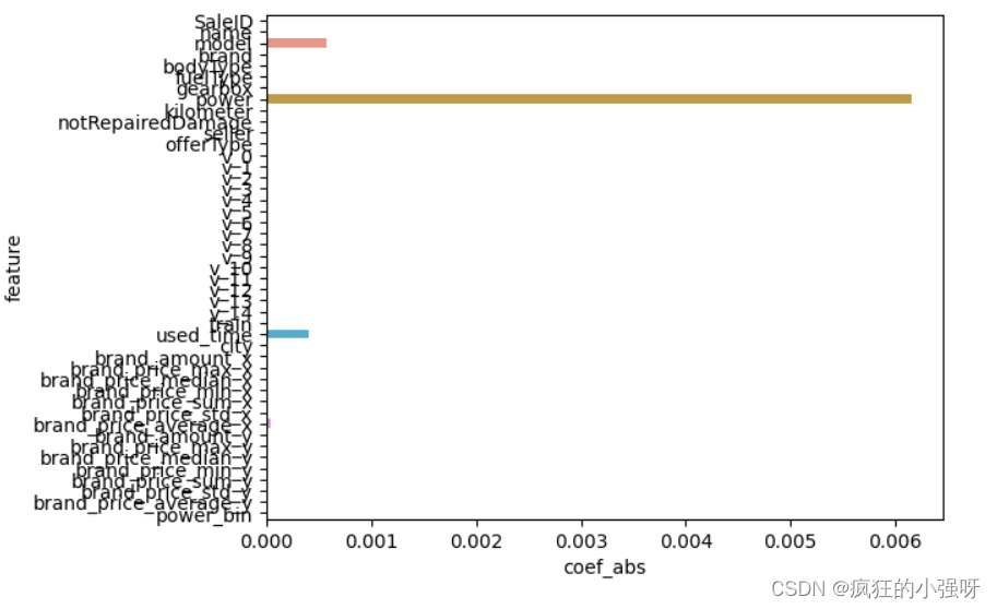
data = pd.DataFrame({'coef_abs': abs(model.coef_), 'feature': train_X.columns})
# 画图
sns.barplot(x='coef_abs', y='feature', data=data)
展示:
- 岭回归
L2正则化在拟合过程中通常都倾向于让权值尽可能小,最后构造一个所有参数都比较小的模型。因为一般认为参数值小的模型比较简单,能适应不同的数据集,也在一定程度上避免了过拟合现象。可以设想一下对于一个线性回归方程,若参数很大,那么只要数据偏移一点点,就会对结果造成很大的影响;但如果参数足够小,数据偏移得多一点也不会对结果造成什么影响,专业一点的说法是『抗扰动能力强』
import seaborn as sns
model = Ridge().fit(train_X, train_y_ln)
print('intercept:', model.intercept_)
# 组合数据
data = pd.DataFrame({'coef_abs': abs(model.coef_), 'feature': train_X.columns})
sns.barplot(x='coef_abs', y='feature', data=data)
展示:
- Lasso回归
L1正则化有助于生成一个稀疏权值矩阵,进而可以用于特征选择
import seaborn as sns
model = Lasso().fit(train_X, train_y_ln)
print('intercept:', model.intercept_)
# 组合数据
data = pd.DataFrame({'coef_abs': abs(model.coef_), 'feature': train_X.columns})
sns.barplot(x='coef_abs', y='feature', data=data)
展示:
在这里我们可以看到power、used_time等特征非常重要
6. 非线性模型
决策树通过信息熵或GINI指数选择分裂节点时,优先选择的分裂特征也更加重要,这同样是一种特征选择的方法。XGBoost与LightGBM模型中的model_importance指标正是基于此计算的
下面我们选择部分模型进行对比:
from sklearn.linear_model import LinearRegression
from sklearn.svm import SVC
from sklearn.tree import DecisionTreeRegressor
from sklearn.ensemble import RandomForestRegressor
from sklearn.ensemble import GradientBoostingRegressor
from sklearn.neural_network import MLPRegressor
from xgboost.sklearn import XGBRegressor
from lightgbm.sklearn import LGBMRegressor
models = [LinearRegression(),DecisionTreeRegressor(),RandomForestRegressor(),GradientBoostingRegressor(),MLPRegressor(solver='lbfgs', max_iter=100), XGBRegressor(n_estimators = 100, objective='reg:squarederror'), LGBMRegressor(n_estimators = 100)]
result = dict()
for model in models:model_name = str(model).split('(')[0]scores = cross_val_score(model, X=train_X, y=train_y_ln, verbose=0, cv = 5, scoring=make_scorer(mean_absolute_error))result[model_name] = scoresprint(model_name + ' is finished')
result = pd.DataFrame(result)
result.index = ['cv' + str(x) for x in range(1, 6)]
result
结果:
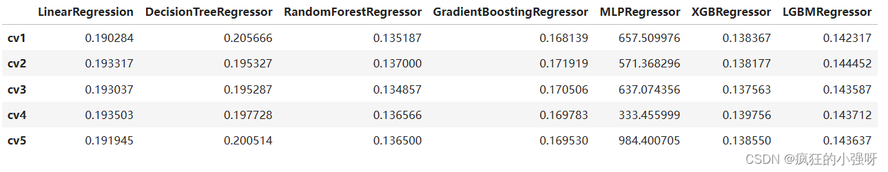
可以看到随机森林模型在每一个fold中均取得了更好的效果!!!
7. 模型调参
在这里主要介绍三种调参方法
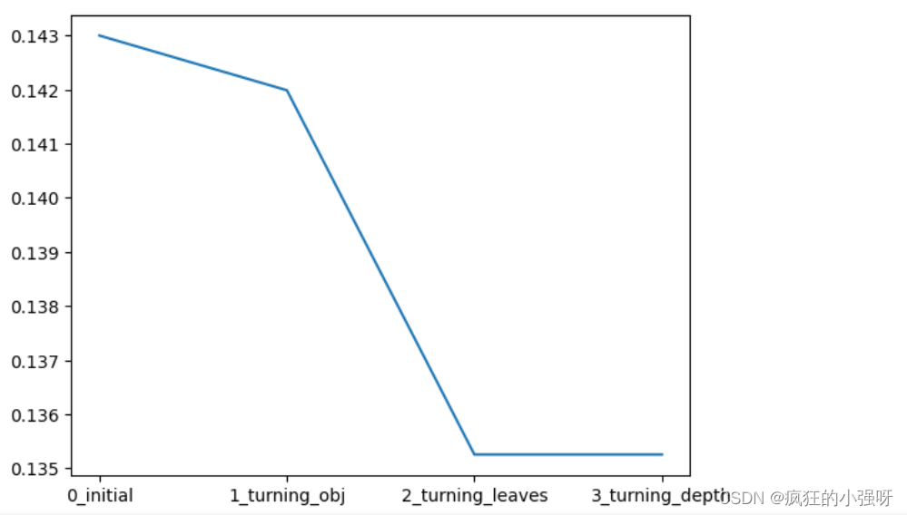
(1) 贪心调参
所谓贪心算法是指,在对问题求解时,总是做出在当前看来是最好的选择。也就是说,不从整体最优上加以考虑,它所做出的仅仅是在某种意义上的局部最优解。
以lightgbm模型为例:
## LGB的参数集合:
# 损失函数
objective = ['regression', 'regression_l1', 'mape', 'huber', 'fair']
# 叶子节点数
num_leaves = [3,5,10,15,20,40, 55]
# 最大深度
max_depth = [3,5,10,15,20,40, 55]
bagging_fraction = []
feature_fraction = []
drop_rate = []
best_obj = dict()
# 计算不同选择下对应结果,其中 score最小时为最优结果
for obj in objective:model = LGBMRegressor(objective=obj)score = np.mean(cross_val_score(model, X=train_X, y=train_y_ln, verbose=0, cv = 5, scoring=make_scorer(mean_absolute_error)))best_obj[obj] = scorebest_leaves = dict()
for leaves in num_leaves:model = LGBMRegressor(objective=min(best_obj.items(), key=lambda x:x[1])[0], num_leaves=leaves)score = np.mean(cross_val_score(model, X=train_X, y=train_y_ln, verbose=0, cv = 5, scoring=make_scorer(mean_absolute_error)))best_leaves[leaves] = scorebest_depth = dict()
for depth in max_depth:model = LGBMRegressor(objective=min(best_obj.items(), key=lambda x:x[1])[0],num_leaves=min(best_leaves.items(), key=lambda x:x[1])[0],max_depth=depth)score = np.mean(cross_val_score(model, X=train_X, y=train_y_ln, verbose=0, cv = 5, scoring=make_scorer(mean_absolute_error)))best_depth[depth] = score
# 画出各选择下,损失的变化
sns.lineplot(x=['0_initial','1_turning_obj','2_turning_leaves','3_turning_depth'], y=[0.143 ,min(best_obj.values()), min(best_leaves.values()), min(best_depth.values())])
(2)Grid Search 调参
GridSearchCV:一种调参的方法,当你算法模型效果不是很好时,可以通过该方法来调整参数,通过循环遍历,尝试每一种参数组合,返回最好的得分值的参数组合
from sklearn.model_selection import GridSearchCV
parameters = {'objective': objective , 'num_leaves': num_leaves, 'max_depth': max_depth}
model = LGBMRegressor()
clf = GridSearchCV(model, parameters, cv=5)
clf = clf.fit(train_X, train_y_ln)
clf.best_params_
得到的最佳参数为:{'max_depth': 10, 'num_leaves': 55, 'objective': 'huber'}
我们再用最佳参数来训练模型:
model = LGBMRegressor(objective='huber',num_leaves=55,max_depth=10)
np.mean(cross_val_score(model, X=train_X, y=train_y_ln, verbose=0, cv = 5, scoring=make_scorer(mean_absolute_error)))
结果跟之前的调参是相当的:
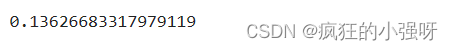
(3)贝叶斯调参
贝叶斯优化通过基于目标函数的过去评估结果建立替代函数(概率模型),来找到最小化目标函数的值。贝叶斯方法与随机或网格搜索的不同之处在于,它在尝试下一组超参数时,会参考之前的评估结果,因此可以省去很多无用功。
from bayes_opt import BayesianOptimization
def rf_cv(num_leaves, max_depth, subsample, min_child_samples):#num_leaves: 决策树上的叶子节点数量。较大的值可以提高模型的复杂度,但也容易导致过拟合。# max_depth: 决策树的最大深度。控制树的深度可以限制模型的复杂度,有助于防止过拟合。# subsample: 训练数据的子样本比例。该参数可以用来控制每次迭代时使用的数据量,有助于加速训练过程并提高模型的泛化能力。# min_child_samples: 每个叶子节点所需的最小样本数。通过限制叶子节点中的样本数量,可以控制树的生长,避免过拟合。val = cross_val_score(LGBMRegressor(objective = 'regression_l1',num_leaves=int(num_leaves),max_depth=int(max_depth),subsample = subsample,min_child_samples = int(min_child_samples)),X=train_X, y=train_y_ln, verbose=0, cv = 5, scoring=make_scorer(mean_absolute_error)).mean()return 1 - valrf_bo = BayesianOptimization(rf_cv,{'num_leaves': (2, 100),'max_depth': (2, 100),'subsample': (0.1, 1),'min_child_samples' : (2, 100)}
)
# 最大化 rf_cv 函数返回的值,即最小化负的平均绝对误差
rf_bo.maximize()
结果:
1 - rf_bo.max['target']
总结
- 上述我们主要通过log转换、正则化、模型选择、参数微调等方法来提高预测的精度
- 最后附上一些学习链接供大家参考:
- 线性回归模型:https://zhuanlan.zhihu.com/p/49480391
- 决策树模型:https://zhuanlan.zhihu.com/p/65304798
- GBDT模型:https://zhuanlan.zhihu.com/p/45145899
- XGBoost模型:https://zhuanlan.zhihu.com/p/86816771
- LightGBM模型:https://zhuanlan.zhihu.com/p/89360721
- 用简单易懂的语言描述「过拟合 overfitting」?https://www.zhihu.com/question/32246256/answer/55320482
- 模型复杂度与模型的泛化能力:http://yangyingming.com/article/434/
- 正则化的直观理解:https://blog.csdn.net/jinping_shi/article/details/52433975
- 贪心算法: https://www.jianshu.com/p/ab89df9759c8
- 网格调参: https://blog.csdn.net/weixin_43172660/article/details/83032029
- 贝叶斯调参: https://blog.csdn.net/linxid/article/details/81189154
相关文章:
数据挖掘入门项目二手交易车价格预测之建模调参
文章目录 目标步骤1. 调整数据类型,减少数据在内存中占用的空间2. 使用线性回归来简单建模3. 五折交叉验证4. 模拟真实业务情况5. 绘制学习率曲线与验证曲线6. 嵌入式特征选择6. 非线性模型7. 模型调参(1) 贪心调参(2)…...
【Java】Java使用Swing实现一个模拟计算器(有源码)
📝个人主页:哈__ 期待您的关注 今天翻了翻之前写的代码,发现自己之前还写了一个计算器,今天把我之前写的代码分享出来。 我记得那会儿刚学不会写,写的乱七八糟,但拿来当期末作业还是不错的哈哈。 直接上…...

MC9S12DJ64微控制器
这份文件是关于Freescale的MC9S12DJ64微控制器的用户指南,包含了关于该设备的详细信息和使用说明。以下是核心内容的整理: 产品信息: 产品信息详细描述如下: 1. **产品名称**:- MC9S12DJ64微控制器单元(MCU)2. **核心…...

小程序打开空白的问题处理
小程序打开是空白的,如下: 这个问题都是请求域名的问题: 一、检查服务器域名配置了 https没有,如果没有,解决办法是申请个ssl证书,具体看这里 https://doc.crmeb.com/mer/mer2/4257 二、完成第一步后&#…...
langchain + azure chatgpt组合配置并运行
首先默认你已经有了azure的账号。 最重要的是选择gpt-35-turbo-instruct模型、api_version:2023-05-15,就这两个参数谷歌我尝试了很久才成功。 我们打开https://portal.azure.com/#home,点击更多服务: 我们点击Azure OpenAI&#…...

【JVM性能调优】- GC调优实操思路
1、GC调优实操思路 前面几点所提及的都是GC调优的一些方法论以及衡量指标,但在真正需要处理GC调优时,上面几点只能给你提供辅导,并不能建立完善的调优思路,因此,接下来再一同论述GC调优的具体实操思想。 GC调优时&…...

四川教育装备行业协会考察团走访云轴科技ZStack共话技术创新应用
近日,四川省教育装备行业协会高等教育技术专业委员会组织了一次深入的考察活动,旨在加强与其他省市高校及企业之间的交流与合作,学习借鉴先进的教育装备与管理经验,以提升本省的高等教育技术水平。考察团一行先后走访了武汉理工大…...
KIVY 学习1
环境 python 3.6 3.7 对应Kivy 1.11.1版本各依赖 python -m pip install docutils pygments pypiwin32 kivy_deps.sdl20.1.22 kivy_deps.glew0.1.12 这是一个用于安装Python包的命令,它会安装一些特定的包。具体来说,这个命令会安装以下包: …...

在Go语言中使用select和channel来期待确定性行为
Go开发人员在使用channel时常犯的一个错误是,对select在多个channel中的行为方式做出错误的假设。错误的假设可能会导致难以识别和重现的细微错误。假设我们要实现一个需要从两个channel接收消息的goroutine: 我们可能会决定像下面这样处理优先级: for {select {case v := &…...
【MATLAB源码-第19期】matlab基于导频的OFDM系统瑞利信道rayleigh的信道估计仿真,输出估计与未估计误码率对比图。
1、算法描述 正交频分复用(英语:Orthogonal frequency-division multiplexing, OFDM)有时又称为分离复频调制技术(英语:discrete multitone modulation, DMT),可以视为多载波传输的一个特例&am…...

坚持十天做完Python入门编程100题第三天加班
坚持十天做完Python入门编程100题第三天加班 第24题 扫描文件列表第25题 如何将字典转换成JSON并写入json文件?第26题 JSON转换成字典 第24题 扫描文件列表 如何扫描当前目录下的文件列表?解析:可以使用python内置的glob模块,用法…...

MSOLSpray:一款针对微软在线账号(AzureO365)的密码喷射与安全测试工具
关于MSOLSpray MSOLSpray是一款针对微软在线账号(Azure/O365)的密码喷射与安全测试工具,在该工具的帮助下,广大研究人员可以直接对目标账户执行安全检测。支持检测的内容包括目标账号凭证是否有效、账号是否启用了MFA、租户账号是…...
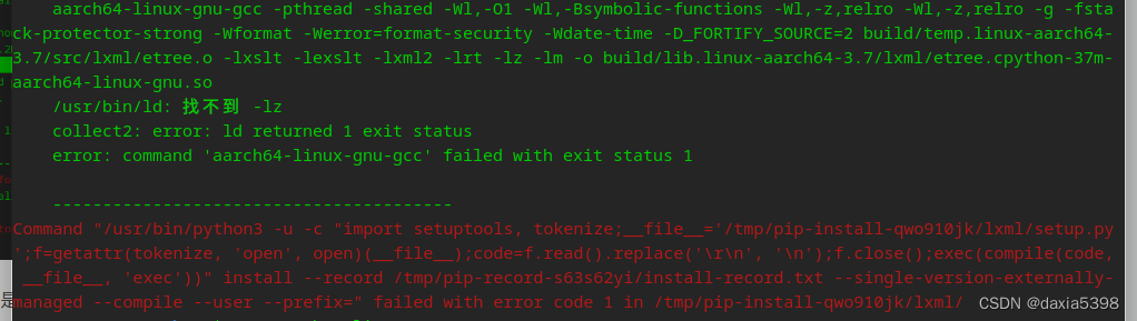
uos安装lxml避坑记录
环境:紫光电脑uos系统 python:系统自带3.7.3 条件:已打开开发者模式,可以自行安装应用商店之外的软件 一、pip3 install lxml4.8.0可以正正常下载,但出现如下错误 另:为什么是4.8.0?因为这个…...
)
518. 零钱兑换 II(力扣LeetCode)
文章目录 518. 零钱兑换 II题目描述动态规划一维数组为什么不能交换两个for循环的顺序? 二维数组 518. 零钱兑换 II 题目描述 给你一个整数数组 coins 表示不同面额的硬币,另给一个整数 amount 表示总金额。 请你计算并返回可以凑成总金额的硬币组合数…...
)
01串的熵(蓝桥杯)
文章目录 01串的熵问题描述答案:11027421题意解释暴力枚举 01串的熵 问题描述 对于一个长度为n的01串 S x 1 x 2 x 3 x_{1}x_{2}x_{3} x1x2x3… x n x_{n} xn,香农信息熵的定义为 H(S) − ∑ 1 n p ( x i ) l o g 2 ( p ( x i ) ) -\sum _{1…...
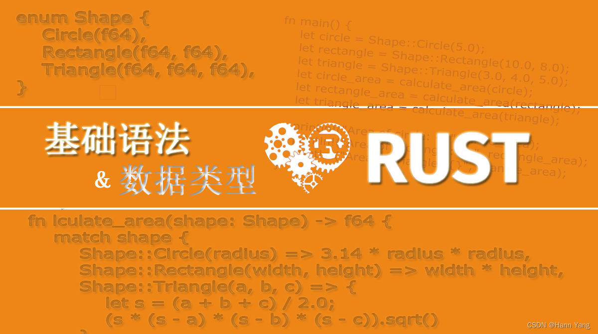
Rust 基础语法和数据类型
数据类型 Rust提供了一系列的基本数据类型,包括整型(如i32、u32)、浮点型(如f32、f64)、布尔类型(bool)和字符类型(char)。此外,Rust还提供了原生数组、元组…...

【Java SE】10 String类
目录 1. String类的重要性 2.常用方法 2.1字符串构造 2.2 String对象的比较 2.3字符串查找 2.4转化 2.5字符串替换 2.6字符串拆分 2.7字符串截取 2.8其他操作方法 2.9字符串的不可变性 2.10字符串修改 3. StringBuffer和StringBuilder 3.1StringBuilder的介绍 4.…...

web蓝桥杯真题:新鲜的蔬菜
代码: .box {display: flex; } #box1 {align-items: center;justify-content: center; }#box2 {justify-content: space-between; } #box2 .item:nth-child(2) {align-self: end; }#box3 {justify-content: space-between; } #box3 .item:nth-child(2) {align-self…...

超声波清洗机能洗哪些东西?洗眼镜超声波清洗机推荐
在现代生活中,人们对清洁卫生的要求越来越高,尤其是对一些细小物件的清洁。眼镜作为我们日常生活中不可或缺的物品,清洁保养更是至关重要。传统的清洗方式可能无法完全清洁眼镜表面的细菌和污垢,于是超声波清洗机成为了很多人的选…...
)
[C++][算法基础]走迷宫(BFS)
给定一个 nm 的二维整数数组,用来表示一个迷宫,数组中只包含 0 或 1,其中 0 表示可以走的路,1 表示不可通过的墙壁。 最初,有一个人位于左上角 (1,1)(1,1) 处,已知该人每次可以向上、下、左、右任意一个方…...

如何一键下载国内主流视频平台的在线视频:Video-Downloader完全指南
如何一键下载国内主流视频平台的在线视频:Video-Downloader完全指南 【免费下载链接】Video-Downloader 下载youku,letv,sohu,tudou,bilibili,acfun,iqiyi等网站分段视频文件,提供mac&win独立App。 项目地址: https://gitcode.com/gh_mirrors/vi/V…...

轻量化之路:使用模型剪枝与量化技术压缩卡证检测模型
轻量化之路:使用模型剪枝与量化技术压缩卡证检测模型 1. 引言 你有没有遇到过这样的场景?想把一个识别身份证、银行卡的AI模型塞进手机App里,或者部署到一台小小的工控机上,结果发现模型动辄几百兆,跑起来慢吞吞&…...

不伤身的酒是智商税?这款轻养新标杆打破偏见
1.当“喝酒伤身”成为共识,谁在挑战这个铁律?中国人喝酒的历史,几乎和文明史一样长。但“喝酒伤身”这四个字,也像影子一样,从未离开过酒桌。每一次举杯,耳边总有人念叨:“少喝点”“伤肝”“伤…...

HsMod终极指南:5步打造你的专属炉石传说模改体验
HsMod终极指南:5步打造你的专属炉石传说模改体验 【免费下载链接】HsMod Hearthstone Modify Based on BepInEx 项目地址: https://gitcode.com/GitHub_Trending/hs/HsMod HsMod是一款基于BepInEx框架的炉石传说模改插件,为玩家提供全面的游戏体验…...
Pixel Dream Workshop 企业级部署架构:基于 Docker 的高可用方案
Pixel Dream Workshop 企业级部署架构:基于 Docker 的高可用方案 1. 为什么企业需要高可用部署方案 当Pixel Dream Workshop从开发测试环境走向生产环境时,稳定性、扩展性和可维护性就成为了关键考量。想象一下,当营销团队急需批量生成节日…...

Linux服务器日志爆满?5个实用命令快速定位并清理大日志文件
Linux服务器日志爆满?5个实用命令快速定位并清理大日志文件 当服务器磁盘空间告急时,日志文件往往是罪魁祸首。作为系统管理员,我们需要快速定位问题并安全清理,避免服务中断。本文将分享5个核心命令的组合使用技巧,帮…...

OFA模型在VMware虚拟机中的开发测试环境搭建
OFA模型在VMware虚拟机中的开发测试环境搭建 对于很多刚接触AI模型开发的个人开发者或学生来说,最大的门槛往往不是算法本身,而是硬件。一块性能足够的独立GPU价格不菲,让很多人在起步阶段就望而却步。难道没有物理GPU,就真的没法…...

SAP移动类型全解析:从收货到移库,一文搞懂库存管理核心配置
SAP移动类型实战指南:解锁库存管理的核心密码 当你第一次在SAP系统中执行货物移动时,面对上百种移动类型代码,是否感到无从下手?作为全球500强企业广泛采用的ERP系统,SAP的库存管理模块以其严谨性和灵活性著称…...

P1095 守望者的逃离【洛谷算法习题】
P1095 守望者的逃离 网页链接 P1095 守望者的逃离 题目背景 NOIP2007 普及组 T3 题目描述 恶魔猎手尤迪安野心勃勃,他背叛了暗夜精灵,率领深藏在海底的娜迦族企图叛变。 守望者在与尤迪安的交锋中遭遇了围杀,被困在一个荒芜的大岛上。…...

从Android大神到AI先锋!10年程序员血泪转型路,AI工程师高薪秘诀全公开!
一眨眼,我已经工作 10 年了。 在 2022 年以前,我一直相信,在这个行业里,只要技术栈钻得深,比如精通三方框架、熟悉 Android Framework、搞定性能优化,就能端稳饭碗。 但从 2023 年开始,一切都变…...